9.5. Blind Handset-Distortion Compensation
As discussed in Section 9.4.2, one popular approach to compensating for handset distortion is to divide handsets into several broad categories according to the type of transducer (e.g., carbon button and electret). During operations, a handset selector is used to identify the most likely handset type from speech signals and handset distortion is compensated for based on some a priori information about the identified type in the database. Although this method works well in landline phones, it may encounter difficulty in mobile handsets because they have a large number of categories, new handset models are frequently released, and models can become obsolete in a short time. Maintaining a handset database for storing the information of all possible handset models is a great challenge and updating the compensation algorithm whenever a new handset is released is also difficult. Therefore, it is imperative to develop a channel compensation method that does not necessarily require a priori knowledge of handsets.
This section describes a blind compensation algorithm for this problem. The algorithm is designed to handle the situation in which no a priori knowledge about the channel is available (i.e., a handset model not in the handset database being used). Because the algorithm does not require a handset selector, it is suitable for a broader scale of deployment than the conventional approaches.
9.5.1. Blind Stochastic Feature Transformation
In speaker verification, it is important to ensure that channel variations are suppressed so that the interspeaker distinction can be enhanced. In particular, given a claimant's utterance recorded in an environment different from that during enrollment, one aims to transform the features of the utterance so that they become compatible with the enrollment environment. Therefore, it is not appropriate to transform the claimant's utterance either to fit the speaker model only or to fit the background model only because the former will result in an unacceptably high FAR (false acceptance rate) and the latter an excessive FRR (false rejection rate). This section describes a feature-based blind transformation approach to solving this problem. The transformation is blind in that it compensates the handset distortion without a priori information about the handset's characteristics. Hereafter, this transformation approach is referred to as blind stochastic feature transformation (BSFT).
Two Phases of BSFT
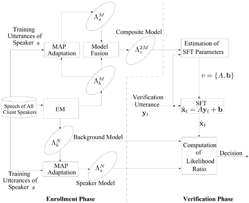
Figure 9.23 illustrates a speaker verification system with BSFT, whose operations are divided into two separate phases: enrollment and verification.
Enrollment Phase. The speech of all client speakers are used to create a compact universal background model (UBM)
 with M components. Then, for each client speaker, a compact speaker model
  is created by adapting the UBM
 using maximum a posteriori (MAP) adaptation [306]. Because verification decisions are based on the likelihood of the speaker model and background model, both models must be considered when the transformation parameters are computed. This can be achieved by fusing
  and
and  to form a 2M-component composite GMM
  . During the fusion process, the means and covariances remain unchanged but the value of each mixing coefficient is divided by 2. This step ensures that the output of the composite GMM represents a probability density function.
Verification Phase. Distorted features Y = {y1, ...,yT} extracted from a verification utterance are used to compute the transformation parameters v = {A, b}. This is achieved by maximizing the likelihood of the composite GMM
 given the transformed features
Equation 9.5.1

where A is a D × D identity matrix for zeroth-order transformation and A = diag{a1, a2, ..., aD} for first-order transformation, and b is a bias vector. The transformed vectors
 are then fed to a full size speaker model
  and a full size UBM
 for computing verification scores in terms of log-likelihood ratio:
Equation 9.5.2

The main idea of BSFT is to transform the distorted features to fit the composite GMM
 , which ensures that the transformation compensates the acoustic distortion.
Figure 9.23. Estimation of BSFT parameters. The background model  , speaker model
  , and composite model
  produced during the enrollment phase, are subsequently used for verification purposes.

A Two-Dimensional Example
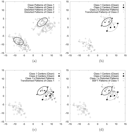
Figure 9.24 illustrates the idea of BSFT in a classification problem with two-dimensional input patterns. Figure 9.24(a) plots the clean and distorted patterns of Class 1 and Class 2. The upper right (respectively lower left) clusters represent the clean (respectively distorted) patterns. The ellipses show the corresponding equal density contours. Markers ♦▪ and represent the centers of the clean models. Figure 9.24(b) illustrates a transformation matching the distorted data of Class 2 and the GMM of Class 1 (GMM1). Because the transformation only takes GMM1 into account, while ignoring GMM2 completely, it results in a high error rate. Similarly, the transformation in Figure 9.24(c) also has a high error rate. The transformation in Figure 9.24(d) was estimated from the distorted data of Class 1 and a composite GMM formed by fusing GMM1 and GMM2. In this case, the transformation adapts the data to a region close to both GMM1 and GMM2 because it takes both GMMs into account. Therefore, instead of transforming the distorted data to a region around GMM1 or GMM2, as in Figures 9.24(b) and 9.24(c), the transformation in Figure 9.24(d) attempts to compensate for the distortion. The capability of BSFT is also demonstrated in a speaker verification task to be described next.
Figure 9.24. A two-class problem illustrating the idea of BSFT. (a) Scatter plots of the clean and distorted patterns corresponding to Class 1 and Class 2. The thick and thin ellipses represent the equal density contours of Class 1 and Class 2, respectively. The upper right (respectively, lower left) clusters contain the clean (respectively, distorted) patterns. (b) Distorted patterns of Class 2 were transformed to fit Class 1's clean model. (c) On the contrary, distorted patterns of Class 1 were transformed to fit Class 2's clean model. (d) Distorted data of Class 1 were transformed to fit a clean, composite model formed by the GMMs of Class 1 and Class 2 (i.e., BSFT). For clarity, only the distorted patterns before and after transformation were plotted in (b) through (d).

Experimental Evaluations
Per the discussion earlier, the experiments were divided into two phases: enrollment and verification.
Enrollment Phase. A 1,024-component UBM
 (i.e., N = 1,024 in Figure 9.23) was trained using the training utterances of all target speakers. The same set of data was also used to train an M-component UBM (
 in Figure 9.23). For each target speaker, a 1,024-component speaker-dependent GMM
 was created by adapting
  using MAP adaptation [306]. Similarly,
  was created by adapting
  , and the two models are fused to form a composite GMM
 . The value of M was varied from 2 to 64 in the experiments.
Verification Phase. For each verification session, a feature sequence Y was extracted from the utterance of a claimant. The sequence was used to determine the BSFT parameters (A and b in Eq. 9.5.1) to obtain a sequence of transformed vectors
 . The transformed vectors were then fed to
  and
and  to obtain verification scores for decision making.
Speech Data and Features
The 2001 NIST speaker recognition evaluation set [151], which contains cellular phone speech of 74 male and 100 female target speakers extracted from the SwitchBoard-II Phase IV Corpus, was used in the evaluations. Each target speaker has 2 minutes of speech for training (i.e., enrollment); a total of 850 male and 1,188 female utterances are available for testing (i.e., verification). Each verification utterance has a length of between 15 and 45 seconds and is evaluated against 11 hypothesized speakers of the same sex as the speaker of the verification utterance. Out of these 11 hypothesized speakers, one is the target speaker who produced the verification utterance. Therefore, there are one target and 10 impostor trials for each verification utterance, which amount to a total of 2,038 target trials and 20,380 impostor attempts for 2,038 verification utterances.
Mel-frequency cepstral coefficients (MFCCs) [69] and their first-order derivatives were computed every 14ms using a Hamming window of 28ms. Cepstral mean subtraction (CMS) [107] was applied to the MFCCs to remove linear channel effects. The MFCCs and delta MFCCs were concatenated to form 24-dimensional feature vectors.
Performance Measures and Results
Detection error tradeoff (DET) curves and equal error rates (EERs) were used as performance measures. They were obtained by pooling all scores of both sexes from the speaker and impostor trials. In addition to DET curves and EERs, a decision cost function (DCF) was also used as a performance measure. The DCF is defined as
![]()
where PTarget and PNontarget are the prior probability of target and impostor speakers, respectively, and where CMiss and CFalseAlarm are the costs of miss and false alarm errors, respectively. Following NIST's recommendation [288], these parameters were set as follows: PTarget = 0.01, PNontarget = 0.99, CMiss = 10, and CFalseAlarm = 1.
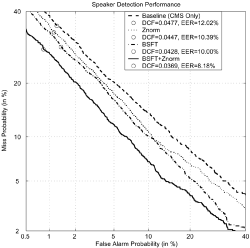
Table 9.16 and Figure 9.25 show the results of the baseline (CMS only), Znorm [14, 303], and BSFT with different order and number of components M in the compact GMMs. Evidently, all cases of BSFT show significant reduction in error rates when compared to the baseline. In particular, Table 9.16 shows that first-order BSFT with Znorm achieves the largest error reduction.[8] The DET curves also show that BSFT with Znorm performs better than the baseline and Znorm for all operating points.
[8] Theoretically, the larger the value of M, the better the results. However, setting M larger than 64 will result in unacceptably long verification time.
Figure 9.25. DET curves comparing speaker verification performance using CMS only (dashed), Znorm (dotted), first-order BSFT without Znorm (dash-dot), and first-order BSFT with Znorm (solid). For the BSFT, the number of components M in the compact GMMs was set to 64. The circles represent the errors at which minimum decision costs occur.

| Compensation Method | SFT Order | M | Equal Error Rate (%) | Minimum Decision Cost |
|---|---|---|---|---|
| Baseline | NA | NA | 12.02 | 0.0477 |
| BSFT | Zeroth | 2 | 11.90 | 0.0473 |
| BSFT | Zeroth | 4 | 11.82 | 0.0458 |
| BSFT | Zeroth | 8 | 11.39 | 0.0449 |
| BSFT | Zeroth | 16 | 11.24 | 0.0450 |
| BSFT | Zeroth | 32 | 11.22 | 0.0450 |
| BSFT | Zeroth | 64 | 11.16 | 0.0443 |
| BSFT | First | 2 | 12.00 | 0.0506 |
| BSFT | First | 4 | 11.55 | 0.0471 |
| BSFT | First | 8 | 10.70 | 0.0464 |
| BSFT | First | 16 | 10.47 | 0.0454 |
| BSFT | First | 32 | 10.43 | 0.0446 |
| BSFT | First | 64 | 10.00 | 0.0428 |
| Znorm | NA | NA | 10.39 | 0.0447 |
| BSFT+Znorm | First | 64 | 8.18 | 0.0369 |
Comparison with Other Models
It is of interest to compare BSFT with the short-time Gaussianization approach proposed in Xiang et al. [387] because both methods transform distorted features in the feature space and their transformation parameters are estimated by the EM algorithm. In short-time Gaussianization, a linear, global transformation matrix is estimated by the EM algorithm using the training data of all background speakers. The global transformation aims to decor-relate the features so that channel variations can be suppressed. The short-time Gaussianization achieves an EER of 10.84% in the NIST 2001 evaluation set [387], whereas BSFT achieves an EER of 9.26%,[9] which represents an error reduction of 14.58%. The minimum decision cost of BSFT is also lower than that of short-time Gaussianization (0.0428 versus 0.0440).
[9] Because Xiang et al. [387] did not use Znorm, their results should be compared with the one without Znorm here.
Computation Consideration
It can be argued that the inferior performance of short-time Gaussianization is due to the nonadaptive nature of its transformation parameters. However, the adaptive nature of BSFT comes with a computational price: different transformation parameters must be computed for each speaker in every verification session. Therefore, it is vital to have a cost-effective computation approach for BSFT. Note that the computation complexity of estimating BSFT parameters grows with the amount of adaptation data (i.e., the value of T in Eq. 9.5.1) and the number of mixture components in the GMMs (i.e., the value of M). To reduce computation time, M should be significantly smaller than N, the number of components in the full size speaker and background models. This is particularly important for the computation of BSFT parameters during the verification phase because the computation time of this phase is a significant part of the overall verification time. The evaluations suggest that a good tradeoff between performance and computation complexity can be achieved by using a suitable value of M.
9.5.2. Integration of Blind and Supervised Compensation
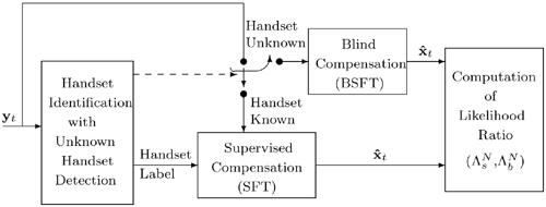
The blind compensation method discussed before is designed to handle handsets that are unknown to the speaker verification system. However, estimating BSFT parameters online requires additional computation during the verification phase. One possible solution to reducing computation without scarifying the advantages of blind compensation is to precompute the transformation parameters of some commonly used handsets and store them in a handset database; during verification, the most appropriate transformation parameters are selected from the database if the handset being used is detected to be one of the a priori known models. In this case, the supervised compensation approach discussed in Section 9.4.2 can be adopted. This paves the way for an integrated approach, combining blind and supervised compensation techniques. Figure 9.26 illustrates how blind and supervised compensation can be integrated into a speaker verification system. This integrated approach can enjoy the best of two worlds: (1) whenever a known handset is detected, precomputed transformation parameters can be used; and (2) should the handset being used be unknown to the system, the system can compute the transformation parameters online using blind or unsupervised techniques.

