
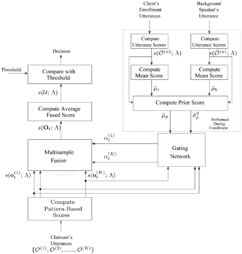
10.4. Multisample Fusion
As discussed in the previous sections, the performance of biometric authentication systems can be improved by the fusion of multiple channels. For example, in Wark and Sridharan [371] and Jourlin et al. [169], the scores from a lip recognizer were fused with those from a speaker recognizer, and in Kittler et al. [182], a face classifier was combined with a voice classifier using a variety of combination rules. These types of systems, however, require multiple sensors, which tend to increase system cost and require extra cooperation from users (e.g., users may need to present their face and utter a sentence to support their claim). Although this requirement can be alleviated by fusing different speech features from the same utterance [330], the effectiveness of this approach relies on the degree of independence among these features.
Another approach to improving the effectiveness of biometric systems is to combine the scores of multiple input samples based on decision-fusion techniques [58,59,223]. Although decision fusion is mainly applied to combine the outputs of modality-dependent classifiers, it can also be applied to fuse decisions or scores from a single modality. The idea is to consider multiple samples extracted from a single modality as independent but coming from the same source. The approach is commonly referred to as multisample fusion [280].
This section investigates the fusion of scores from multiple utterances to improve the performance of speaker verification from GSM-transcoded speech. The simplest way of achieving this goal is to average the scores obtained from multiple utterances, as in Poh et al. [280]. Although score averaging is a reasonable approach to combining the scores, it gives equal weight to the contribution of speech patterns from multiple utterances, which may not produce optimal fused scores. In light of this deficiency, computing the optimal fusion weights based on the score distribution of the utterances and on prior score statistics determined from enrollment data [223] was recently proposed. To further enhance the effectiveness of the proposed fusion algorithm, prior score statistics are to be adapted during verification, based on the probability that the claimant is an impostor [58]. This is called data-dependent decision fusion (DF). Because the variation of handset characteristics and the encoding/decoding process introduce substantial distortion to speech signals [397], stochastic feature transformation [226] was also applied to the feature vectors extracted from the GSM-transcoded speech before presenting them to the clean speaker model and background model.
10.4.1. Data-Dependent Decision Fusion Model
Architecture
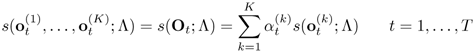
Assume that K streams of features vectors (e.g., MFCCs [69]) can be extracted from K-independent utterances u = {u1,..., uk}. The observation sequence corresponding to utterance uk is denoted by
Equation 10.4.1
![]()
where D and Tk are the dimensionality of ![]() and the number of observations in O(k), respectively. A normalized score function [215] is defined as
and the number of observations in O(k), respectively. A normalized score function [215] is defined as
Equation 10.4.2
![]()
where Λ = {Λwc, Λwb} contains the Gaussian mixture models (GMMs) that characterize the client speaker (wc) and the background speakers (wb), and log p![]() is the output of GMM Λw, w ε {wc, wb}, given observation
is the output of GMM Λw, w ε {wc, wb}, given observation ![]() .
.
The expert-in-class architecture [190] is an ideal candidate for combining normalized scores probabilistically. Specifically, frame-level fused scores are computed according to
Equation 10.4.3
where ![]() represents the confidence (reliability) of the observation
represents the confidence (reliability) of the observation ![]() and
and ![]() . The mean fused score
. The mean fused score
Equation 10.4.4
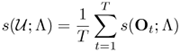
is compared against a decision threshold to make verification decisions. For nota-tional convenience, the K utterances are assumed to contain the same number of feature vectors. If not, the tail of the longer utterances can be appended to the tail of the shorter ones to make the number of feature vectors equal. In Eq. 10.4.3, a larger (respectively smaller) fusion weight means a greater (respectively lesser) influence on the final decision. Fusion weights can be estimated using training data; alternatively, they can be determined purely from the observation data during recognition. Rather than using either training data or recognition data exclusively, a new approach in which the fusion weights depend on both training data (prior information) and recognition data is proposed.
During enrollment, the mean score of each client speaker ![]() and of the background speakers
and of the background speakers ![]() are determined. Then, the overall mean score
are determined. Then, the overall mean score
Equation 10.4.5
![]()
is used as the prior score for that client. In Eq. 10.4.5, Kc and Kb are the numbers of client speaker's utterances and background speakers' utterances, respectively. A prior variance
Equation 10.4.6
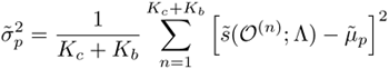
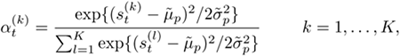
is also to be computed, where ![]() denotes the mean score of the n-th utterance. Then, during verification, the claimant is asked to utter K utterances, and the fusion weights are computed according to
denotes the mean score of the n-th utterance. Then, during verification, the claimant is asked to utter K utterances, and the fusion weights are computed according to
Equation 10.4.7
where for ease of presentation, ![]() has been defined. Figure 10.6 depicts the architecture of the fusion model.
has been defined. Figure 10.6 depicts the architecture of the fusion model.
Theoretical Analysis
The following theoretical analysis of the fusion algorithm explains how and why it achieves better performance than the equal-weight fusion approach does.
Figure 10.7(a) illustrates the fusion weights ![]() as a function of
as a function of ![]() and
and ![]() where
where ![]() ∊ [−12, 12], k ∊ {1,2},
∊ [−12, 12], k ∊ {1,2}, ![]() , and
, and ![]() . A closer look at Figure 10.7(a) reveals that scores falling on the upper-right region of the dashed line L are increased by the fusion function Eq. 10.4.3. This is because in that region, for
. A closer look at Figure 10.7(a) reveals that scores falling on the upper-right region of the dashed line L are increased by the fusion function Eq. 10.4.3. This is because in that region, for ![]() ,
, ![]() and
and ![]() ; moreover, for
; moreover, for ![]() ,
, ![]() and
and ![]() . Both of these conditions make Eq. 10.4.3 emphasize the larger score. Conversely, the fusion algorithm puts more emphasis on the small scores if they fall on the lower-left region of the dashed line. The effect of the fusion weights on the scores is depicted in Figure 10.7(b). Evidently, the fusion weights favor large scores if they fall on the upper-right region, whereas the fused scores are close to the small scores if they fall on the lower-left region.
. Both of these conditions make Eq. 10.4.3 emphasize the larger score. Conversely, the fusion algorithm puts more emphasis on the small scores if they fall on the lower-left region of the dashed line. The effect of the fusion weights on the scores is depicted in Figure 10.7(b). Evidently, the fusion weights favor large scores if they fall on the upper-right region, whereas the fused scores are close to the small scores if they fall on the lower-left region.
Figure 10.7. (a) Fusion weights  as a function of scores
  and
and  . (b) Contour plot of fused scores based on the fusion formula in Eq. 10.4.3 and the fusion weights in (a).

The rationale behind this fusion approach is the observation that most client-speaker scores are larger than the prior score, but most of the impostor scores are smaller than the prior score. As a result, if the claimant is a client speaker, the fusion algorithm favors large scores; on the other hand, the algorithm favors small scores if the claimant is an impostor. This has the effect of reducing the overlapping area of score distribution of client speakers and impostors, thus reducing the error rate.
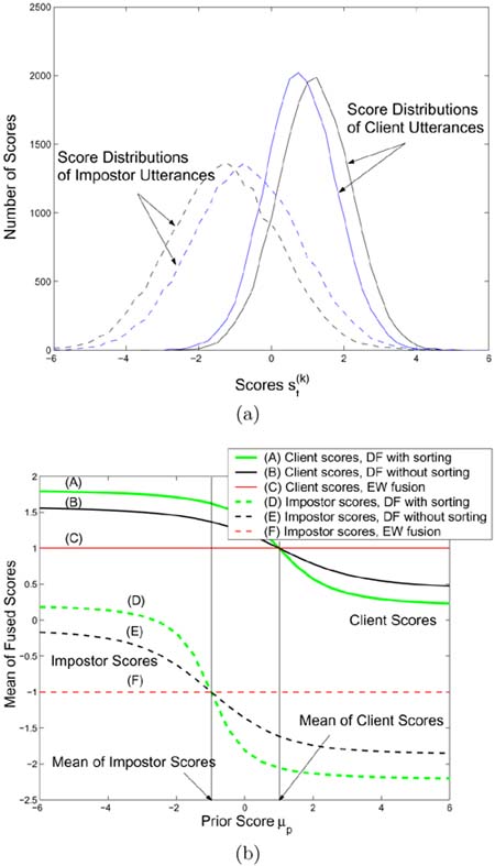
Gaussian Example
Figure 10.8 shows an example where the distributions of client speaker scores and impostor scores are assumed to be Gaussian. It is also assumed that both the client and the impostor produce two utterances. The client speaker's mean scores for the first and second utterances are equal to 1.2 and 0.8, respectively. Likewise, the impostor's mean scores for the two utterances are equal to −1.3 and −0.7. Obviously, equal-weight (EW) fusion produces a mean speaker score of 1.0 and a mean impostor score of −1.0, resulting in a score dispersion of 2.0. These two mean scores (− 1.0 and 1.0) are indicated by the two vertical lines in Figure 10.8(b). Figures 10.8(b) and 10.8(c) show that when the prior score ![]() is set to a value between these two means (i.e., between the vertical lines), the data-dependent fusion (DF) algorithm can produce a score dispersion larger than 2.0. As the mean of fused scores is used to make the final decision, increasing the score dispersion can decrease the speaker verification error rate.
is set to a value between these two means (i.e., between the vertical lines), the data-dependent fusion (DF) algorithm can produce a score dispersion larger than 2.0. As the mean of fused scores is used to make the final decision, increasing the score dispersion can decrease the speaker verification error rate.
Figure 10.8. (a) Distributions of client scores and impostor scores as a result of four utterances: 2 from a client speaker and another 2 from an impostor; the means of client scores are 0.8 and 1.2, and the means of impostor scores are −1.3 and −0.7; (b) mean of fused client scores and the mean of fused impostor scores; and (c) difference between the mean of fused client scores and the mean of fused impostor scores based on EW fusion and DF with and without score sorting.

10.4.2. Fusion of Sorted Scores
Because the fusion model described in Section 10.4.1 depends on pattern-based scores of individual utterances, the positions of scores in the score sequences can also affect the final fused scores. The scores in the score sequences can be sorted before fusion such that small scores will always be fused with large scores [59]. This is achieved by sorting half of the score sequences in ascending order and the other half in descending order. The fusion of sorted scores applies only to even numbers of utterances.
Theoretical Analysis
The Gaussian example can be used to extend the theoretical analysis in Section 10.4.1 to explain why the fusion of sorted scores is better than the fusion of unsorted scores.
In the analysis described in Section 10.4.1, the increase or decrease of the mean fused scores is probabilistic only because there is no guarantee that the scores of the two utterances (![]() ,
, ![]() ) ∀t fall in either the upper-right region or the lower-left region of the score space together. In many cases, some of the (
) ∀t fall in either the upper-right region or the lower-left region of the score space together. In many cases, some of the (![]() ,
, ![]() ) pairs fall in the region above Line L in Figure 10.7 and others in the region below it, even though the two utterances are obtained from the same speaker. This situation is undesirable because it introduces uncertainty to the increase or decrease of the mean fused scores. This uncertainty, however, can be removed by sorting the two score sequences before fusion takes place because the scores to be fused will always lie on a straight line. For example, if the mean scores of both utterances from the client speaker are denoted as μ, and the
) pairs fall in the region above Line L in Figure 10.7 and others in the region below it, even though the two utterances are obtained from the same speaker. This situation is undesirable because it introduces uncertainty to the increase or decrease of the mean fused scores. This uncertainty, however, can be removed by sorting the two score sequences before fusion takes place because the scores to be fused will always lie on a straight line. For example, if the mean scores of both utterances from the client speaker are denoted as μ, and the ![]() is assumed to be sorted in ascending order and
is assumed to be sorted in ascending order and ![]() in descending order, the relationship
in descending order, the relationship ![]() results. This is the straight line
results. This is the straight line ![]() shown in Figure 10.7, when μ = 1. Evidently, Line L1 lies in the region where large scores are emphasized. As a result, an increase in the mean fused score can be guaranteed.
shown in Figure 10.7, when μ = 1. Evidently, Line L1 lies in the region where large scores are emphasized. As a result, an increase in the mean fused score can be guaranteed.
Numerical Example
A numerical example is used here to demonstrate the effect of sorting scores. Figure 10.9 shows a hypothetical situation in which scores were obtained from two client utterances. For client utterances, Eq. 10.4.7 should emphasize large scores and deemphasize small scores. However, Figure 10.9(a) illustrates the situation in which a very small score (5th score of utterance 2—i.e., −‐2) is fused with a relatively large score (5th score of utterance 1—i.e., 0.0). In this case, ![]() and
and ![]() , which means the fifth fused score ( − 1.76) is dominated by the fifth score of utterance 2. This is undesirable for client utterances.
, which means the fifth fused score ( − 1.76) is dominated by the fifth score of utterance 2. This is undesirable for client utterances.
Figure 10.9. Fused scores derived from unsorted (left) and sorted (right) score sequences obtained from a client speaker. The assumption is that  and
and  in Eq. 10.4.7.
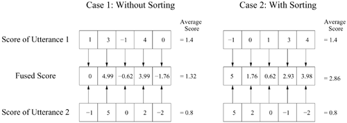
The influence of those extremely small client scores on the mean fused score can be reduced by sorting the scores of the two utterances in opposite order before fusion such that small scores will always be fused with large scores. With this arrangement, the contribution of extremely small client scores in one utterance can be compensated for by the large scores of another utterance. As a result, the mean of the fused client scores is increased.
Figure 10.9(b) shows that the mean of fused scores is increased from 1.32 to 2.86 after the scores are sorted. Likewise, if this sorting approach is applied to the scores of impostor utterances with proper prior scores μp (i.e., greater than the mean of impostor scores—see Figure 10.8(b)), the contribution of extremely large impostor scores in one utterance can be greatly reduced by the small scores in another utterance, which has the net effect of minimizing the mean of the fused impostor scores. Therefore, this score sorting approach can further increase the dispersion between client scores and impostor scores, as shown in Figure 10.8(c). This has the effect of lowering the error rate.
Effect on Real Speech Data
To further demonstrate the merit of sorting the scores before fusion, two client speakers (faem0 and mdac0) were selected from the handset TIMIT (HTIMIT) corpus, and the distributions of the fused speaker scores and fused impostor scores were plotted in Figure 10.10. In Eq. 10.4.7, the overall mean ![]() was used as the prior score. However, as the number of background speakers' utterances is much larger than that of the speaker's utterances during the training phase, the overall mean is very close to the mean score of the background speakers
was used as the prior score. However, as the number of background speakers' utterances is much larger than that of the speaker's utterances during the training phase, the overall mean is very close to the mean score of the background speakers ![]() —that is,
—that is, ![]() . Therefore, according to Section 10.4.2, the mean of fused impostor scores remains almost unchanged, but the mean of fused client scores increases significantly. Figure 10.10(a) shows that the mean of client scores increases from 0.35 to 1.08 and the mean of impostor scores decreases from −3.45 to −3.59 after sorting the score sequences. The decrease in the mean of fused impostor scores is caused by the prior score
. Therefore, according to Section 10.4.2, the mean of fused impostor scores remains almost unchanged, but the mean of fused client scores increases significantly. Figure 10.10(a) shows that the mean of client scores increases from 0.35 to 1.08 and the mean of impostor scores decreases from −3.45 to −3.59 after sorting the score sequences. The decrease in the mean of fused impostor scores is caused by the prior score ![]() being greater than the mean of the unfused impostor scores—see the fourth figure in Figure 10.10(a). Thus, the dispersion between the mean client score and the mean impostor score increases from 3.80 to 4.67.
being greater than the mean of the unfused impostor scores—see the fourth figure in Figure 10.10(a). Thus, the dispersion between the mean client score and the mean impostor score increases from 3.80 to 4.67.
Figure 10.10. Distribution of pattern-by-pattern client (top) and impostor scores (second), the mean of fused client and fused impostor scores (third), and difference between the mean of fused client and fused impostor scores (bottom) based on EW fusion (score averaging) and DF with and without score sorting. The means of speaker and impostor scores obtained by both fusion approaches are also shown.

Figure 10.10(b) reveals that both the mean of client scores and the mean of impostor scores increase. This is because the means of impostor scores obtained from verification utterances are greater than the prior score ![]() , thus resulting in the increase of the mean of fused impostor scores. However, because the increase in the mean client scores is still greater than the increase in the mean impostor scores, there is a net increase in the score dispersion. Specifically, the dispersion in Figure 10.10(b) increases from 2.14 (= 0.24− (−1.90)) to 2.63 (= 0.94− (−1.69)). Because verification decision is based on the mean scores, the wider the dispersion between the mean client scores and the mean impostor scores, the lower the error rate.
, thus resulting in the increase of the mean of fused impostor scores. However, because the increase in the mean client scores is still greater than the increase in the mean impostor scores, there is a net increase in the score dispersion. Specifically, the dispersion in Figure 10.10(b) increases from 2.14 (= 0.24− (−1.90)) to 2.63 (= 0.94− (−1.69)). Because verification decision is based on the mean scores, the wider the dispersion between the mean client scores and the mean impostor scores, the lower the error rate.
10.4.3. Adaptation of Prior Scores
Eq. 10.4.7 uses the overall mean ![]() as the prior score. However, because the number of background speakers' utterances is much larger than the number of the speaker's utterances during the training phase, the overall mean is very close to the mean score of the background speakers (i.e.,
as the prior score. However, because the number of background speakers' utterances is much larger than the number of the speaker's utterances during the training phase, the overall mean is very close to the mean score of the background speakers (i.e., ![]() ). This causes most of the client speaker scores to be larger than the prior score; moreover, only part of the impostor scores are smaller than the prior score. An example of this situation is illustrated in Figure 10.11 in which the distributions of the pattern-by-pattern speaker scores and impostor scores corresponding to speaker mdac0 are shown. Figures 10.7 and 10.11 show that if the claimant is a client speaker, the fusion algorithm favors large scores because most of the speaker scores in Figure 10.11 are larger than the prior score. On the other hand, the algorithm has equal preference on both small and large scores if the claimant is an impostor because the prior score is in the middle of the impostor scores' distribution.
). This causes most of the client speaker scores to be larger than the prior score; moreover, only part of the impostor scores are smaller than the prior score. An example of this situation is illustrated in Figure 10.11 in which the distributions of the pattern-by-pattern speaker scores and impostor scores corresponding to speaker mdac0 are shown. Figures 10.7 and 10.11 show that if the claimant is a client speaker, the fusion algorithm favors large scores because most of the speaker scores in Figure 10.11 are larger than the prior score. On the other hand, the algorithm has equal preference on both small and large scores if the claimant is an impostor because the prior score is in the middle of the impostor scores' distribution.
Figure 10.11. Distribution of pattern-by-pattern speaker and impostor scores corresponding to speaker mdac0. Most of the speaker scores are larger than the prior score, and only some of the impostor scores are smaller than the prior score.
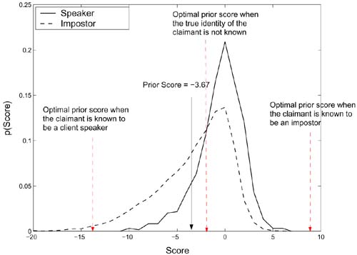
The ultimate goal of Eq. 10.4.7 is to favor large scores when the claimant is a client speaker; on the other hand, if the claimant is an impostor, the fusion algorithm should favor small scores. In other words, the goal is to increase the separation between client speakers' scores and impostors' scores. As a result, when the claimant is a true speaker, the prior score should be smaller than all possible speaker scores so that Eq. 10.4.7 favors only larger scores; on the other hand, when the claimant is an impostor, the prior score should be larger than all possible impostor scores so that Eq. 10.4.7 favors only smaller scores. However, satisfying these two conditions simultaneously is almost impossible in practice because the true identity of the claimant is never known. Therefore, the optimal prior score should be equal to the intersection point of speaker score distribution and impostor score distribution (see Figure 10.11). At that point, the number of speaker scores smaller than the prior score plus the number of impostor scores larger than the prior score is kept to a minimum.
Adaptation Algorithm
A method to adapt the prior score during verification in order to achieve the goal mentioned before [58] follows. For each client speaker, a one-dimensional GMM score model Ωscore with output
Equation 10.4.8
is trained to represent the distribution of the utterance-based background speakers' scores ![]() s(ot;Λ) obtained during the training phase. During verification, a claimant is asked to utter K utterances u = {u1,..., uk}. For the k-th utterance, the normalized likelihood that the claimant is an impostor is computed
s(ot;Λ) obtained during the training phase. During verification, a claimant is asked to utter K utterances u = {u1,..., uk}. For the k-th utterance, the normalized likelihood that the claimant is an impostor is computed
Equation 10.4.9
where ![]() s(ot;Λ) is the score of the k-th utterance. The prior score is then adapted according to
s(ot;Λ) is the score of the k-th utterance. The prior score is then adapted according to
Equation 10.4.10
![]()
where ![]() is the adapted prior score and f(ζ) is a monotonic increasing function controlling the amount of adaption. Then,
is the adapted prior score and f(ζ) is a monotonic increasing function controlling the amount of adaption. Then, ![]() in Eq. 10.4.7 is replaced by
in Eq. 10.4.7 is replaced by ![]() to compute the fusion weights. The reason for using a monotonic function for f(ζ) is that if the normalized likelihood of a claimant is large, he or she is likely to be an impostor. As a result, the prior score should be increased by a large amount to deemphasize the high scores of this claimant. With the large scores being deemphasized, the claimant's mean fused score becomes smaller, thus increasing the chance of rejecting this potential impostor.
to compute the fusion weights. The reason for using a monotonic function for f(ζ) is that if the normalized likelihood of a claimant is large, he or she is likely to be an impostor. As a result, the prior score should be increased by a large amount to deemphasize the high scores of this claimant. With the large scores being deemphasized, the claimant's mean fused score becomes smaller, thus increasing the chance of rejecting this potential impostor.
Notice that Eq. 10.4.10 increases the prior score rather than decreasing it because the optimal prior score is always greater than the unadapted prior score ![]() . A monotonic function of the form is used,
. A monotonic function of the form is used,
Equation 10.4.11
![]()
where a represents the maximum amount of adaptation and b controls the rate of increase of f(ζ) with respect to ζ. Figure 10.12 shows the effect of varying a and b on the adapted prior scores, where the larger the normalized likelihood, the greater the degree of adaption. This is reasonable because a large normalized likelihood means the claimant is likely to be an impostor; as a result, the prior score should be increased by a greater amount to deemphasize the large scores of this claimant. With the large scores being deemphasized, the claimant's mean fused score becomes smaller, thus increasing the chance of rejecting this potential impostor.
Figure 10.12. The influence of varying a and b of Eq. 10.4.10 on the adapted prior scores  , assuming that
  =−5.
=−5.

Effect of Score Adaptation on Score Distributions
To demonstrate the effect of the proposed prior score adaptation on fused score distributions, a client speaker (mdac0) from GSM-transcoded HTIMIT was arbitrarily selected and the distributions of the fused speaker scores and fused impostor scores were plotted in Figure 10.13, using EW fusion (![]() =
= ![]() = 0.5 ∀t), DF without prior score adaptation (Eq. 10.4.7), and DF with prior score adaptation (Eq. 10.4.10). Evidently, the upper part of Figure 10.13 shows that the number of large client speaker scores is greater in data-dependent fusion, and the lower part of Figure 10.13 shows that there are more small impostor scores in DF than in EW fusion. The figure also shows that data-dependent fusion with prior score adaptation outperforms the other two fusion approaches.
= 0.5 ∀t), DF without prior score adaptation (Eq. 10.4.7), and DF with prior score adaptation (Eq. 10.4.10). Evidently, the upper part of Figure 10.13 shows that the number of large client speaker scores is greater in data-dependent fusion, and the lower part of Figure 10.13 shows that there are more small impostor scores in DF than in EW fusion. The figure also shows that data-dependent fusion with prior score adaptation outperforms the other two fusion approaches.
Figure 10.13. Distribution of pattern-by-pattern (a) speaker scores and (b) impostor scores based on EW fusion (score averaging) and DF. Solid: equal-weight fusion. Thin dotted: data-dependent fusion without prior score adaptation. Thick dotted: Data-dependent fusion with prior score adaptation.
Further evidence demonstrating the advantage of prior score adaptation can be found in Table 10.1. In particular, Table 10.1 shows that the dispersion between the mean client score and the mean impostor score increases from 2.63 (= −0.53 − (−3.16)) to 4.04 (= 0.25 − (−3.79)) without prior score adaptation and to 4.61 (= 0.22 − (−4.39)) with prior score adaptation. Because verification decisions are based on the mean scores, the wider the dispersion between the mean client scores and the mean impostor scores, the lower the error rate. Table 10.1 also shows that with prior score adaptation, both the mean speaker score and mean impostor score are reduced. The reason for a reduction in the mean speaker score is that there is a small increase in the prior score when the claimant is a true speaker, which increases the number of scores that are smaller than the prior score. In other words, more small speaker scores are emphasized by Eq. 10.4.7, which lowers the fused speaker scores as well as the mean speaker score.
| Equal Weight | Fusion without PS Adaptation | Fusion with PS Adaptation | |
|---|---|---|---|
| Prior score | N/A | -3.67 | Vary for different utterances |
| Mean speaker score | -0.53 | 0.25 | 0.22 |
| Mean impostor score | -3.16 | -3.79 | -4.39 |
| Score dispersion | 2.63 | 4.04 | 4.61 |
10.4.4. Experiments and Results
The multisample fusion techniques described before were applied to a speaker verification task. This section details the experimental setup and discusses the results obtained.
Experiments on Multisample Fusion and Score Sorting
Data Sets and Feature Extraction
The HTIMIT corpus (see Reynolds [304]) was used in the experiments. Handset TIMIT was obtained by playing a subset of the TIMIT corpus through nine phone handsets and a Sennheizer head-mounted microphone. A GSM speech coder [91] transcoded the HTIMIT corpus and the data-dependent fusion techniques were applied to the resynthesized coded speech. In the sequel, the two corpora are denoted as HTIMIT and GSM-HTIMIT.
Speakers in HTIMIT were divided into two sets: speaker set and impostor set, as shown in Table 10.2. Similar to the speakers in HTIMIT, speakers in GSM-HTIMIT were also divided into two sets; the speaker identities (arranged alphabetically) of these sets are identical to those in HTIMIT. Twelve mel-frequency cepstrum coefficients (MFCCs) [69] were extracted from the utterances every 14ms using a 28ms Hamming window.
| Set | Speaker Name |
|---|---|
| Speaker set (50 male, 50 female) | fadg0, faem0, ... , fdxw0; mabw0, majc0, ... , mfgk0; mjls0, mjma0, mjmd0, mjmm0, mpdf0 |
| Impostor set (25 male, 25 female) | feac0, fear0, . . . , fjem0; mfxv0, mgaw0, . . . , mjlg1 |
| Pseudo-impostor set I (10 male, 10 female) | fjen0, fjhk0, . . . , fjrp1; mjpm1, mjrh0, . . . , mpgr1 |
| Pseudo-impostor set II (50 male, 50 female) | fjen0, fjhk0, ... , fmbg0; mjpm1, mjrh0, ... , msrr0 |
Enrollment Procedures
During enrollment, the SA and SX utterances from handset "senh" of the uncoded HTIMIT were used to create a 32-center GMM for each speaker. A 64-center universal background GMM [306] was also created based on the speech of 100 client speakers recorded from handset "senh." The background model will be shared among all client speakers in subsequent verification sessions.
Besides the speaker models and the background model, a two-center GMM (Λx in Section 9.4.2) was created using the uncoded HTIMIT utterances (from handset senh) of 10 speakers. A set of transformation parameters (bi's in Section 9.4.1) were then estimated using this model and the handset- and codec-distorted speech (see Section 9.4.2).
Verification Procedures
For verification, the GSM-transcoded speech from all 10 handsets in HTIMIT was used. As a result, there were handset and coder mismatches between the speaker models and verification utterances. Stochastic feature transformation with handset identification [226, 227, 352] was used to compensate for the mismatches.
The SI sentences in the corpora were used for verification, and each claimant was asked to utter two sentences during a verification session (i.e., K = 2 in Eq. 10.4.1). To obtain the scores of the claimant's utterances, the utterances were first fed to a handset selector [226] to determine the set of feature transformation parameters to be used. The features were transformed and then fed to the claimed speaker model and the background model to obtain the normalized scores (see Eq. 10.4.2). Next, the data-dependent fusion algorithms were applied to fuse two independent streams of scores. Since different utterances contain different numbers of feature vectors, two utterances must have an identical number of feature vectors (length) before fusion takes place. In this work, this length was calculated according to
Equation 10.4.12
![]()
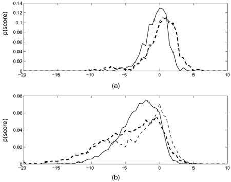
where L is a positive integer, and L1 and L2 represent the length of the first and second utterance, respectively. Figure 10.14 illustrates how the length equalization is performed; there are 105 and 138 feature vectors in the first and second utterance, respectively. According to Eq. 10.4.12, the equal length is 121 (= [(105+138)/2]). After finding the equal length, the remaining scores in the longer utterance (Utterance 2 in this case) are appended to the end of the shorter utterance (Utterance 1 in this case). In this example, one extra score in Utterance 2 is discarded to make the length of the two utterances equal.
Figure 10.14. Procedure for making equal-length utterances: (a) before and (b) after length equalization. The tail of the longer utterance is appended to the tail of the shorter one.
To compare with EW fusion proposed by [280], the utterances' scores were also fused using equal fusion weights (i.e., ![]() =
= ![]() = 0.5 ∀t = 1, ..., L).
= 0.5 ∀t = 1, ..., L).
Results and Discussion
Figure 10.15 depicts the detection error tradeoff (DET) curves based on 100 client speakers and 50 impostors using utterances from Handset cb1 for verification. Figure 10.15 clearly shows that with feature transformation, data-dependent fusion can reduce error rates significantly, and sorting the scores before fusion can reduce the error rate even further. However, without feature transformation, the performance of DF with score sorting is not significantly better than that of EW fusion. This is caused by the mismatch between the prior scores ![]() 's in Eq. 10.4.7 and the scores of the distorted features. Therefore, it is very important to use feature transformation to reduce the mismatch between the enrollment data and verification data.
's in Eq. 10.4.7 and the scores of the distorted features. Therefore, it is very important to use feature transformation to reduce the mismatch between the enrollment data and verification data.
Figure 10.15. DET curves for EW fusion (score averaging) and DF with and without score sorting. The curves were obtained by using the utterances of Handset cb1 as verification speech.
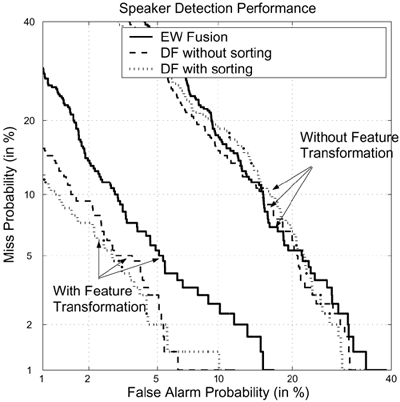
Table 10.3 shows the speaker detection performance of 100 client speakers and 50 impostors for the EW fusion approach and the proposed fusion approach with and without sorting the score sequences. Table 10.3 also clearly shows that the proposed fusion approach outperforms the equal-weight fusion. In particular, after sorting the score sequences, the equal error rates are further reduced. Compared to the unsorted cases, an 11% error reduction has been achieved.
| Fusion Method | Equal Error Rate (%) | ||||||||||
|---|---|---|---|---|---|---|---|---|---|---|---|
| cbl | cb2 | cb3 | cb4 | ell | e12 | e13 | e14 | pt1 | senh | Ave. | |
| No fusion (single utterance) | 6.31 | 6.36 | 19.96 | 15.35 | 5.89 | 10.83 | 11.79 | 8.18 | 9.38 | 4.90 | 9.90 |
| EW fusion | 5.11 | 4.33 | 19.15 | 12.89 | 4.42 | 8.31 | 9.96 | 6.29 | 7.57 | 2.99 | 8.10 |
| DF without sorting | 4.01 | 3.27 | 15.92 | 10.55 | 3.04 | 6.51 | 8.67 | 4.75 | 7.51 | 2.32 | 6.67 |
| DF with sorting | 3.60 | 2.86 | 15.30 | 9.91 | 3.49 | 4.65 | 6.81 | 4.02 | 6.59 | 1.99 | 5.92 |
Experiments on Score Adaptation
Similar to the preceding experiments, HTIMIT and GSM-transcoded HTIMIT were used in the experiments. Speakers in HTIMIT were divided into four sets, as shown in Table 10.2. The pseudo-impostor sets in Table 10.2 were used to train the impostor score model (the one-dimensional GMM mentioned in Section 10.4.3) that characterizes the pseudo-impostor scores. The output of this model was used to adapt the prior score, as detailed in Section 10.4.3.
Two sets of pseudo-impostor scores were collected. For the first set, the SA and SX utterances of all speakers in the speaker set were fed to the background model and each of the speaker models to obtain the pseudo-impostor scores corresponding to the enrollment data. For the second set, the utterances of all speakers in the pseudo-impostor sets were fed to the background model and each of the speaker models to obtain the pseudo-impostor scores corresponding to unseen impostor data. These pseudo-impostor scores were averaged for each utterance. The resulting utterance-based scores were used to create a two-center one-dimensional GMM pseudo-impostor score model (Ωscore in Section 10.4.3).
Optimizing the Adaptation Parameters
In the experiments, the parameters a and b in Eq. 10.4.10 were set to 10 and 5, respectively. These values were empirically found to obtain reasonably good results; that is, parameters a and b would probably not be too large. If a is too large (e.g., a = 20 in Figure 10.12), Eq. 10.4.10 leads to a large adapted prior score ![]() even for utterances with a low normalized likelihood ζ. As a result, almost all of the claimant scores will become smaller than the prior score, which is undesirable. Moreover, a large a will result in poor verification performance when there is a lot of mismatch between the pseudo-impostor score model and the verification scores because, in a severe mismatch situation, Eq. 10.4.9 will produce an incorrect normalized likelihood. This leads to incorrect adaptation of the prior score, which in turn results in incorrect fusion weights. On the other hand, if b is too large, there will be a sharp bend in the adaptation curves, as illustrated in Figure 10.12. As a result, the prior score is adapted only when the verification utterances give a high likelihood in Eq. 10.4.9. The best range for parameter a is 5 to 20 and for parameter b, it is 5 to 8.
even for utterances with a low normalized likelihood ζ. As a result, almost all of the claimant scores will become smaller than the prior score, which is undesirable. Moreover, a large a will result in poor verification performance when there is a lot of mismatch between the pseudo-impostor score model and the verification scores because, in a severe mismatch situation, Eq. 10.4.9 will produce an incorrect normalized likelihood. This leads to incorrect adaptation of the prior score, which in turn results in incorrect fusion weights. On the other hand, if b is too large, there will be a sharp bend in the adaptation curves, as illustrated in Figure 10.12. As a result, the prior score is adapted only when the verification utterances give a high likelihood in Eq. 10.4.9. The best range for parameter a is 5 to 20 and for parameter b, it is 5 to 8.
Results and Discussion
Figure 10.16 depicts the speaker detection performance based on 100 speakers and 50 impostors for the equal-weight fusion (score averaging) approach and the proposed fusion approach. Figure 10.16 clearly shows that with feature transformation, DF is able to reduce error rates significantly. In particular, with feature transformation, the EER achieved by data-dependent fusion with prior score adaptation is 4.01%. When compared to EW fusion, which achieves an EER of 5.11%, a relative error reduction of 22% was obtained.
Figure 10.16. Speaker detection performance for EW fusion (score averaging) and DF.

In Figure 10.16, the speakers in the speaker-set were used to train the pseudo-impostor score model. The distribution of pseudo-impostor scores obtained from unseen data are of interest and are illustrated in Figure 10.17. By comparing Figure 10.17(a) with Figure 10.17(c), it is obvious that there is a mismatch between the pseudo-impostor score distribution and impostor score distribution. In particular, there are more small scores in Figure 10.17(a) than in Figure 10.17(c). This mismatch affects the adaptation of prior scores because the likelihood ζ in Eq. 10.4.9 is no longer accurate. This is evident in Table 10.4 where the EERs using different numbers of pseudo-impostors with speech extracting from different corpora are shown. In particular, the last column of Table 10.4 clearly shows that the improvement after adapting the prior scores is just 3.14% (from 4.14% to 4.01%).
| PI-20 GSM | PI-100 GSM | PI-100 HTIMIT | SS-100 HTIMIT | |
|---|---|---|---|---|
| DF with PS adaptation (a = 20) | 2.80% (2.78%) | 2.57% (2.71%) | 4.22% (4.23%) | 4.05% (3.69%) |
| DF with PS adaptation (a = 10) | 3.01% (2.55%) | 2.92% (2.25%) | 3.68% (3.51%) | 4.01% (3.60%) |
| DF without PS adaptation | 3.61% (2.81%) | 3.52% (2.67%) | 3.92% (3.80%) | 4.14% (3.60%) |
| EW fusion | 5.11% | 5.11% | 5.11% | 5.11% |
| No fusion (single utterance) | 6.31% | 6.31% | 6.31% | 6.31% |
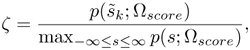
Figure 10.17. Distribution of pseudo-impostor scores for speaker fadg0 obtained by using (a) HTIMIT speech in the speaker set and (b) GSM-transcoded speech in the pseudo-impostor set. (c) Distribution of impostor scores for speaker fadg0 during verification using GSM-transcoded speech.

In Table 10.4, the values inside the parentheses indicate the EERs obtained from different fusion approaches with score sorting. Each figure is based on the average of 100 speakers, each impersonated by 50 impostors. The abbreviations in the first row of the table denote the data used for creating the pseudo-impostor score model, as follows:
PI-20 GSM: Pseudo-impostor set containing 20 speakers, with GSM-transcoded speech from Handset cb1
PI-100 GSM: Pseudo-impostor set containing 100 speakers, with GSM-transcoded speech from Handset cb1
PI-100 HTIMIT: Pseudo-impostor set containing 100 speakers, with HTIMIT speech from Handset senh
SS-100 HTIMIT: Speaker set containing 100 speakers, with HTIMIT speech from Handset senh
To create a more stable and reliable pseudo-impostor score model, another set of speakers (the pseudo-impostor set) was used to train the pseudo-impostor score model. In addition, GSM-transcoded speech, instead of HTIMIT speech, was used to train the model in an attempt to create a verification environment as close to the real one as possible. The GSM-transcoded speech was transformed before calculating the scores. Figures 10.17(b) and 10.17(c) show that the score distributions are much closer after using the transformed features. The improvement after adapting the prior score is 17% (from 3.52% to 2.92%), as demonstrated in the second column of Table 10.4.
Table 10.4 shows that even for a pseudo-impostor set containing as few as 20 speakers, a lower EER (3.01%) can still be obtained by using the GSM-transcoded speech to train the pseudo-impostor score model. System performance can be further improved from 3.01% to 2.55% by applying the prior score adaptation together with score sorting.
By using the GSM-transcoded speech, the real verification environment can be modeled so that parameter a can be increased to obtain a much lower EER (from 3.01% to 2.80% when using 20 pseudo-impostors and from 2.92% to 2.57% when using 100 pseudo-impostors). However, the error rate increases from 3.68% to 4.22% and from 4.01% to 4.05% when there is a mismatch between the pseudo-impostor score distribution and the pseudo-impostor score model. As the fusion weights are an exponential function of the distance between the individual scores and the prior score, Eq. 10.4.7 puts more emphasis on small scores if the prior score increases. Therefore, if the claimant is an impostor, the mean impostor score becomes smaller. On the other hand, if the prior score is wrongly adapted, the mean speaker score also becomes smaller because there are more scores smaller than the prior score. Figure 10.12 shows that for the same likelihood, the increase in prior scores is larger when parameter a is increased from 10 to 20. In other words, even if inaccurate likelihood is obtained, its influence on system performance is small when parameter a is small. Therefore, if a stable and reliable pseudo-impostor score distribution is obtained, parameter a can be increased to further improve verification performance. This step is taken because if an utterance gives high likelihood in Eq. 10.4.9, the claimant is more likely to be an impostor; Eq. 10.4.7 can then be made to emphasize only small scores. On the other hand, when an utterance gives low likelihood in Eq. 10.4.9, the prior score should be increased slightly so that it is close to the optimal prior score (see Figure 10.11), because impostors' utterances can also give low likelihood. The parameter a should be kept small so that system performance is not degraded when a stable and reliable pseudo-impostor score model cannot be obtained.
Large-Scale Evaluations
Data Sets and Feature Extraction
To further demonstrate the capability of DF under practical situations, evaluations were performed using cellular phone speech: the 2001 NIST speaker recognition evaluation set [151], which consists of 174 target speakers (clients), 74 male and 100 female. Another set of 60 speakers is also available for development. Each target speaker has 2 minutes of speech for training, and the duration of each test speech varies from 15 to 45 seconds. The set provides a total of 20,380 gender-matched verification trials. The ratio between target and impostor trials is roughly 1:10.
Twelve MFCCs and their first-order derivative were extracted from the utterances every 14ms using a Hamming window of 28ms. These coefficients were concatenated to form a 24-dimensional feature vector. Cepstral mean subtraction (CMS) [107] was applied to remove linear channel effects.
Enrollment Procedure
A 1024-component universal GMM background model [306] was created based on the speech of all 174 client speakers. A speaker-dependent GMM was then created for each client speaker by adapting the universal background model using maximum a posteriori (MAP) adaptation [306]. Finally, all 60 speakers in the development set were used to create a two-center one-dimensional GMM pseudo-impostor score model (Ωscore in Section 10.4.3).
Verification Procedures
For each verification session, a test sentence was first fed to the claimed speaker model and the universal background model to obtain a sequence of normalized scores. The average of these scores was then used for decision making. This traditional method (referred to as the EW approach) is the baseline. In addition to the equal-weight approach, the proposed fusion algorithm was applied to compute the weight of each score. Because only one test utterance exists for each verification session, the utterance was split into two segments and then fusion was performed. In this case, the length was calculated according to
Equation 10.4.13
![]()
where T is a positive integer and L represents the length of the test utterance.
Performance Measure
In addition to detection error tradeoff (DET) curves and equal error rates, another performance measure for the NIST evaluations is the detection cost function (DCF), which is defined as follows:
Equation 10.4.14
![]()
where Pr(I) and Pr(T) are the prior probability of impostor and target speaker, respectively, and where CFA and CFR are the specific cost factors for false alarm and false rejection, respectively. In this work, Pr(I) = 0.99, Pr(T) = 0.01, CFA = 1 and CFR = 10 were set as recommended by the NIST.
Optimizing the Adaptation Parameters
In the HTIMIT experiments, the parameters a and b in Eq. 10.4.10 were fixed for each speaker. However, in this experiment, a full search method and a set of training data were used to determine the best value of a and b for each client speaker. By feeding a set of pseudo-impostors into a client model, a set of mean fused pseudo-impostor scores were obtained. All 60 speakers in the development set of NIST 2001 were used as the pseudo-impostors. With different values of a and b, different sets of mean fused pseudo-impostor scores were obtained. More precisely, a particular set of a and b results in 60 mean pseudo-impostor scores. Similarly, by feeding the client speech into his or her own model and varying a and b, different mean fused client scores are obtained.
In this experiment, because there was only one utterance for training a client model, only one mean fused client score was obtained for a particular value of a and b. The value of a and b were chosen to
Minimize the number of mean fused pseudo-impostor scores that are greater than the mean fused client scores.
Maximize the difference between the mean fused client score and the largest mean fused pseudo-impostor scores provided that the mean fused client score is larger than the largest mean fused pseudo-impostor scores.
The search range of a is 0 to 10 and b is 3 to 8. The HTIMIT experiments demonstrated that a cannot be too large and b cannot be too small; otherwise, a large mismatch between the pseudo-impostor score model and the verification scores may result in poorer performance.
Results and Discussion
Figure 10.18 depicts the speaker detection performance for the DF approach with different values of a and b. According to Figure 10.12, when a and b are fixed to 10 and 3, respectively, the adapted prior scores are very large, even for small normalized likelihood ζ. This large degree of adaptation of prior scores leads to a reduction in the mean fused client scores. As a result, the miss probability (FRR) becomes larger than without adaptation when the false alarm probability is higher than 13%, as illustrated in Figure 10.18. On the other hand, when a is fixed to 10 and b is fixed to 8, there is a sharp bend in the adaptation curves (see Figure 10.12). Thus, the prior score is adapted only if the verification utterances give a high likelihood in Eq. 10.4.9, and the performance is just slightly better than without prior scores adaptation. Figure 10.18 shows that the best performance is achieved when the full search method is used to determine the value of a and b.
Figure 10.18. Speaker detection performance for DF with and without prior score adaptation.
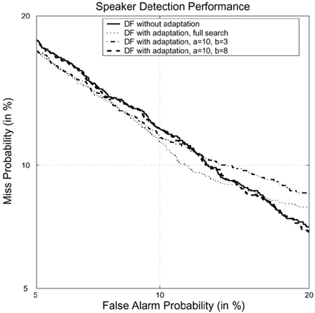
Figure 10.19 depicts the speaker detection performance of the EW fusion approach and the proposed fusion approach (with the parameters a and b obtained by full search). The figure clearly shows that data-dependent fusion reduces error rates. The EER achieved by DF with prior score adaptation is 10.50%. When compared to EW fusion (which achieves an EER of 12.05%), a relative error reduction of 13% was obtained. Data-dependent fusion with prior score adaptation achieves a 4% improvement as compared to the baseline in terms of minimum DCF.
Figure 10.19. Speaker detection performance for baseline (score averaging) and DF. Adaptation parameters a and b were obtained by the full search method.
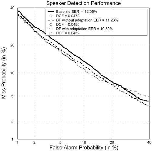
Nevertheless, DF with prior score adaptation has a disadvantage. Figure 10.19 shows that when the false alarm probability is higher than 20%, the performance of data-dependent fusion with prior score adaptation degrades. This phenomenon, which is caused by the large degree of adaptation of the prior scores even for client speakers, decreases the mean fused client scores, resulting in the rejection of more client speakers. However, the proposed algorithm is much preferred for those systems that require low false alarm probability. At low false alarm probability, the proposed fusion algorithm can achieve a lower miss probability as compared to the EW fusion approach.
Figure 10.19 shows that splitting an utterance into two segments and fusing their pattern-based scores can achieve a performance that is better than the result of considering the utterance as only a single segment. Table 10.5 depicts the EERs and minimum detection cost obtained by splitting the verification utterances into different numbers of segments followed by the fusion algorithms. Splitting a verification utterance into two to five segments can achieve a performance better than simply taking the average of all scores (i.e., the EW approach). A much lower DCF can also be obtained by splitting the utterances into three segments—0.0442 for DF with prior score adaptation and 0.0445 for DF without prior score adaptation. These represent a 6.36% and 5.72% reduction in DCF with respect to the baseline.
| DF without PS Adaptation | DF with PS Adaptation | |||
|---|---|---|---|---|
| No. of segments | EER | DCF | EER | DCF |
| K = 1 (Equal Weight) | 12.05% | 0.0472 | 12.05% | 0.0472 |
| K = 2 | 11.23% | 0.0455 | 10.50% | 0.0452 |
| K = 3 | 10.89% | 0.0445 | 10.50% | 0.0442 |
| K = 4 | 10.96% | 0.0449 | 10.56% | 0.0446 |
| K = 5 | 11.10% | 0.0459 | 10.55% | 0.0450 |