Chapter 5. Functions
Functions are preprogrammed mini-programs that perform a certain task. As with mathematics, functions transform values into another result. SQL Server 2005 has a wide range of built-in functions to carry out various tasks. In this chapter, we introduce several of SQL Server 2005’s useful built-in functions, which can be divided into row-level functions, aggregate functions, and other special functions. Row-level functions operate on a row at a time, whereas aggregate functions operate on many rows at once.
In SQL Server, we can group the row-level functions into four types: numeric functions, string functions, conversion functions, and date functions. Numeric functions are used for calculations. An example of a numeric function is the SQUARE function, which would return the square (a row at a time) of every number (row) of a particular column. String functions are used to manipulate strings in a particular column (again, one row at a time). An example of a string function is SUBSTRING, which extracts characters from a string. Conversion functions are used to convert a particular column (a row at a time) from one data type to another. And, date functions (created using the DATETIME data type) operate on a particular data column or attribute, a row at a time. Date functions are also considered fundamental to the operations of a database.
The second category of functions that we will discuss is aggregate functions. Aggregate functions provide a one-number result after calculations based on multiple rows. Examples of aggregate functions are MIN or AVG, which stand for the minimum or average, respectively, and return the minimum or average value respectively, of multiple rows of a particular column.
The third category of functions that we will discuss is a special class of “other” functions. These other functions produce a smaller subset of rows from multiple rows. Example of these other kind of functions would be the DISTINCT function or the TOP function, both of which produce a smaller subset of rows from the complete set.
Note that most of the functions discussed in this chapter are placed in a SELECT statement, and so they are “read-only” or “display-only” functions. Any SELECT statement function will not change the underlying data in the database. To change the underlying data in a database, UPDATE (instead of SELECT) would have to be used (as shown in Chapter 3).
We begin the chapter by discussing aggregate functions. We discuss row-level functions later in the chapter.
Aggregate Functions
An aggregate function (or group function) is a function that returns a result (one number) after calculations based on multiple rows. We use the term “aggregate” (instead of “group”), because it avoids confusion later in the book (we discuss other GROUP functions in Chapter 9). An aggregate function basically combines multiple rows into a single number. Aggregate functions can be used to count the number of rows, find the sum or average of all the values in a given numeric column, and find the largest or smallest of the entries in a given column. In SQL, these aggregate functions are: COUNT,
SUM, AVG, MAX, and MIN, respectively. In this section, we examine several of these aggregate functions.
The COUNT Function
The COUNT function is used to count how many (rows) of something there are, or the number of rows in a result set. Following is the general syntax for the COUNT function.
    SELECT COUNT(*)
    FROM   Table-name(s)
COUNT(*) returns a count of the number of rows in the table(s).
The following query counts the number of rows in the table, Grade_report:
    SELECT COUNT(*) AS [Count]
    FROM   Grade_report
The following is its output:
    Count
    -----------
    209

    (1 row(s) affected)
COUNT(*) counts all rows, including rows that have some (or even all) null values in some columns.
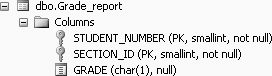
In Figure 5-1, we present the table definition of the Grade_report table to remind you of the columns available in the Grade_report table.
Sometimes we want to count how many items we have in a specific column. The general syntax for counting the number of items in a specific column is:
    SELECT COUNT(attribute_name)
    FROM   Table-name(s)
For example, to count the number of grades in the grade column of the Grade_report table, we could type the following:
    SELECT COUNT(grade) AS [Count of Grade]
    FROM   Grade_report
This produces the following output:
    Count of Grade
    --------------
    114

    (1 row(s) affected)
COUNT(column) counts only non null columns. Although the Grade_report table has 209 rows, you get a count of 114 grades rather than 209 grades, because there are some null grades in the grade column.
The COUNT feature can be quite useful because it can save you from unexpectedly long results. Also, you can use it to answer “how many” queries without looking at the row-values themselves. In Chapter 4, which showed how Cartesian products are generated, you learned that SQL does not prevent programmers from asking questions that have very long or even meaningless answers. Thus, when dealing with larger tables, it is good to first ask the question, “How many rows can I expect in my answer?” This question may be vital if a printout is involved. For example, consider the question, “How many rows are there in the Cartesian product of the Student, Section, and Grade_report tables in our database?” This is answered by the query:
    SELECT COUNT(*) AS Count
    FROM   Student, Section, Grade_report
The following output shows the count from this query, which will be equal to the product of the table sizes of the three tables (the Cartesian product of the three tables). Obviously, in this example, it would be a good idea to first find out the number of rows in this result set before printing it.
    Count
    -----------
    321024

    (1 row(s) affected)
Contrast the previous COUNTing-query and its Cartesian product result to this query:
    SELECT  COUNT(*) AS [Count]
    FROM    Student, Grade_report, Section
    WHERE   Student.stno = Grade_report.student_number
    AND     Grade_report.section_id  = Section.section_id
The following is the result of this query:
    Count
    -----------
    209

    (1 row(s) affected)
What is requested here is a count of a three-way equi-join rather than a three-way Cartesian product, the result of which is something you probably would be much more willing to work with. Note also that you expect a count of about 209 from the sizes of the tables involved: Student (48 rows), Grade_report (209 rows), and Section (32 rows). The expected count of a join operation is of the order of magnitude of the larger number of rows in the tables.
SQL syntax will not allow you to count two or more columns at the same time. The following query will not work:
    SELECT COUNT (grade, section_id)
    FROM   Grade_report
You will get the following error message:
    Msg 174, Level 15, State 1, Line 2
    The COUNT function requires 1 argument(s).
The SUM Function
The SUM function totals the values in a numeric column. For example, suppose you have another table called Employee that looks like this:
    names           wage         hours
    --------------- ------------ -----------
    Sumon Bagui     10.0000      40
    Sudip Bagui     15.0000      30
    Priyashi Saha   18.0000      NULL
    Ed Evans        NULL         10
    Genny George    20.0000      40

    (5 row(s) affected)
In this Employee table, names is defined as a NVARCHAR column, wage is defined as a SMALLMONEY column, and hours is defined as SMALLINT.
Tip
This Employee table has not been created for you in the Student_course database. You have to create and insert rows into it in order to run the following queries.
To find the sum of hours worked, use the SUM function like this:
    SELECT SUM(Hours) AS [Total hours]
    FROM   Employee
This query produces the following output:
    Total hours
    ---------------------
    120

    Warning: Null value is eliminated by an aggregate or other SET operation.
    (1 row(s) affected)
Columns that contain null values are not included in the SUM function (and not in any aggregate numeric functions except COUNT(*)).
The AVG Function
The AVG function calculates the arithmetic mean (the sum of non null values divided by the number of non null values) of a set of values contained in a numeric column (or attribute) in the result set of a query. For example, if you want to find the average hours worked from the Employee table, type:
    SELECT AVG(hours) AS [Average hours]
    FROM   Employee
This produces the following output:
    Average hours
    ---------------------
    30

    Warning: Null value is eliminated by an aggregate or other SET operation.
    (1 row(s) affected)
Again, note that the null value is ignored (not used) in the calculation of the average, so the total hours (120) is divided by 4 rather than 5.
The MIN and MAX Functions
The MIN function finds the minimum value from a column, and the MAX function finds the maximum value (once again, nulls are ignored). For example, to find the minimum and maximum wage from the Employee table, you could type the following:
    SELECT MIN(wage) AS [Minimum Wage], MAX(wage) AS [Maximum Wage]
    FROM   Employee
This query produces the following output:
    Minimum Wage Maximum Wage
    ------------ ------------
    20.0000

    Warning: Null value is eliminated by an aggregate or other SET operation.
    (1 row(s) affected)
The MIN and MAX functions also work with character and datetime columns. For example, if we type:
    SELECT "First name in alphabetical order" = MIN(names)
    FROM   Employee
We will get:
    First name in alphabetical order
    --------------------------------
    Ed Evans

    (1 row(s) affected)
And, if we type:
    SELECT "Last name in alphabetical order" = MAX(names)
    FROM   Employee
We will get:
    Last name in alphabetical order
    -------------------------------
    Sumon Bagui

    (1 row(s) affected)
In the case of strings, the MIN and MAX are related to the collating sequence of the letters in the string. Internally, the column that we are trying to determine the MIN or MAX of is sorted alphabetically. Then, MIN returns the first (top) of the alphabetical list, and MAX returns the last (bottom) of the alphabetical list.
Row-Level Functions
Whereas aggregate functions operate on multiple rows for a result, row-level functions
operate on values in single rows, one row at a time. In this section, we look at row-level functions that are used in calculations—for example, row-level functions that are used to add a number to a column, the ROUND function, the ISNULL function, and others.
Arithmetic Operations on a Column
A row-level “function” can be used to perform an arithmetic operation on a column.
Tip
Strictly speaking a row-level “function” is not a function, but an operation performed in a result set. But the use of arithmetic operations in result sets behaves like functions.
For example, in the Employee table, if we wanted to display every person’s wage plus 5, we could type the following:
    SELECT wage, (wage + 5) AS [wage + 5]
    FROM   Employee
In this query, from the Employee table, first the wage is displayed, then the wage is incremented by five with (wage + 5), and displayed.
This query produces the following output:
    wage         wage + 5
    ------------ ------------
    10.0000      15.0000
    15.0000      20.0000
    18.0000      23.0000
    NULL         NULL
    20.0000      25.0000

    (5 row(s) affected)
Tip
Similarly, values can be subtracted (with the - operator), multiplied (with the * operator), and divided (with the / operator) to and from columns.
Once again, note that (wage + 5) is only a “read-only” or “display-only” function, because we are using it in a SELECT statement. The wage in the Employee table is not actually changing. We are only displaying what the wage + 5 is. To actually increase the wage in the Employee table by 5, we would have to use the UPDATE command. Any other arithmetic operation may be performed on numeric data.
The ROUND Function
The ROUND function rounds numbers to a specified number of decimal places. For example, in the Employee table, if you wanted to divide every person’s wage by 3 (a third of the wage), you would type (wage/3). Then, to round this, you could use ROUND(wage/3), and include the precision (number of decimal places) after the comma. In query form, this would be:
    SELECT names, wage, ROUND((wage/3), 2) AS [wage/3]
    FROM   Employee
This query produces the following output:
    names                wage                  wage/3
    -------------------- --------------------- ---------------------
    Sumon Bagui          10.00                 3.33
    Sudip Bagui          15.00                 5.00
    Priyashi Saha        18.00                 6.00
    Ed Evans             NULL                  NULL
    Genny George         20.00                 6.67

    (5 row(s) affected)
In this example, the values of (wage/3) are rounded up to two decimal places because of the “2” after the comma after ROUND(wage/3).
Other Common Numeric Functions
Other very common numeric functions include:
CEILING(attribute), which returns the next larger integer value when a number contains decimal places.FLOOR(attribute), which returns the next lower integer value when a number contains decimal places.SQRT(attribute), which returns the square root of positive numeric values.ABS(attribute), which returns the absolute value of any numeric value.SQUARE(attribute), which returns a number squared.
The ISNULL Function
The results of the queries in the preceding sections show not only that nulls are ignored, but that if a null is contained in a calculation on a row, the result is always null. We will illustrate, with a couple of examples, how to handle this NULL issue.
Example 1
In the first example, we will illustrate how to handle the NULL problem and also illustrate how to create variables on the fly. SQL Server 2005 allows you to create variables on the fly using a DECLARE statement followed by a @, the variable name (a or b, in our example) and then data type of the variable (both declared as FLOAT in our example). Variables are assigned values using the SET statement. And variables can be added in the SELECT statement.
So, type the following sequence to declare the variables (a and b), assign values to them, and then add them together:
    DECLARE @a FLOAT, @b FLOAT
    SET @a = 3
    SET @b = 2
    SELECT @a + @b AS 'A + B = '
This query gives the result:
    A + B =
    ----------------
    5

    (1 row(s) affected)
SQL Server allows the use of SELECT with no FROM clause for such calculations as we have illustrated.
Now, if you set the variable a to null, as follows:
    DECLARE @a FLOAT, @b FLOAT
    SET @a = NULL
    SET @b = 2
    SELECT @a + @b AS 'A + B = '
You get this:
    A + B =
    ----------------
    NULL

    (1 row(s) affected)
To handle the null issue, SQL Server 2005 provides a row-level function, ISNULL, which returns a value if a table value is null. The ISNULL function has the following form:
ISNULL(expression1, ValueIfNull)
The ISNULL function says that if the expression (or column value) is not null, return the value, but if the value is null, return ValueIfNull. Note that the ValueIfNull must be compatible with the data type. For example, if you wanted to use a default value of zero for a null in the previous example, you could type this:
    DECLARE @a FLOAT, @b FLOAT
    SET @a = NULL
    SET @b = 2
    SELECT ISNULL(@a, 0) + ISNULL(@b, 0) AS 'A + B = '
Which would give:
    A + B =
    -----------------
    2

    (1 row(s) affected)
Here, @b is unaffected, but @a is set to zero for the result set as a result of the ISNULL function. @a is not actually changed, it is replaced for the purposes of the query.
Example 2
For the second example we will use the Employee table. To multiply the wage by hours and avoid the null-result problem by making the nulls act like zeros, a query could read:
    SELECT names, wage, hours, ISNULL(wage, 0)*ISNULL(hours,0) AS [wage*hours]
    FROM   Employee
This query would produce the following output:
    names           wage         hours       wage*hours
    --------------- ------------ ----------- ------------
    Sumon Bagui     10.00         40          400.00
    Sudip Bagui     15.00         30          450.00
    Priyashi Saha   18.00         NULL        0.00
    Ed Evans        NULL          10          0.00
    Genny George    20.00         40          800.00

    (5 row(s) affected)
ISNULL does not have to have a ValueIfNull equal to zero. For example, if you want to assume that the number of hours is 40 if the value for hours is null, then you could use the following expression:
    SELECT names, wage, new_wage = ISNULL(wage, 40)
    FROM   Employee
This query would give:
    names           wage         new_wage
    --------------- ------------ ------------
    Sumon Bagui     10.00        10.00
    Sudip Bagui     15.00        15.00
    Priyashi Saha   18.00        18.00
    Ed Evans        NULL         40.00
    Genny George    20.00        20.00

    (5 row(s) affected)
The NULLIF Function
SQL Server 2005 also has a NULLIF function, which returns a NULL if expression1
=
expression2. If the expressions are not equal, then expression1 is returned. The NULLIF function has the following form:
NULLIF(expression1,expression2)
For example, if we want to see whether the wage is 0, we would type:
    SELECT names, wage, new_wage = NULLIF(wage, 0)
    FROM   Employee
This query would give:
    names           wage         new_wage
    --------------- ------------ ------------
    Sumon Bagui     10.00        10.00
    Sudip Bagui     15.00        15.00
    Priyashi Saha   18.00        18.00
    Ed Evans        NULL         NULL
    Genny George    20.00        20.00

    (5 row(s) affected)
From these results we can see that because none of the wages are equal to 0, the wage (expression1) is returned in every case. Even the NULL wage (Ed Evans’s wage) is not equal to 0, but NULL is returned anyway, as the value in question is NULL.
If, for example, a wage 15 was unacceptable for some reason, you could null out the value of 15 using the NULLIF function like this:
    SELECT names, wage,
           new_wage = NULLIF(wage, 15)
    FROM   Employee
This query would give:
    names           wage         new_wage
    --------------- ------------ ------------
    Sumon Bagui     10.00        10.00
    Sudip Bagui     15.00        NULL
    Priyashi Saha   18.00        18.00
    Ed Evans        NULL         NULL
    Genny George    20.00        20.00

    (5 row(s) affected)
Again, as can be noted from the previous set of results, you have to be very careful about the interpretation of the output obtained from a NULLIF function if there were already nulls present in the columns being tested. Ed Evans’s wage was not equal to15, but had a NULL originally (and this may be wrongly interpreted when the NULLIF function is being used).
Other Row-Level Functions
Other row-level functions in SQL Server 2005 include ABS, which returns the absolute value of a numeric expression. For example, if we wanted to find the absolute value of -999.99, we could type the following:
SELECT ABS(-999.99) AS [Absolute Value]
This query would produce the following output:
    Absolute Value
    --------------
    999.99

    (1 row(s) affected)
There are also several other row-level trigonometric functions available in Server SQL 2005, including SIN, COS, TAN, LOG, and so forth. But, as these functions are less commonly used, we will not discuss them.
Other Functions
This section discusses some other useful functions, such as TOP,
TOP with PERCENT, and DISTINCT. These functions help us in selecting rows from a larger set of rows.
The TOP Function
This function returns a certain number of rows. Often, the TOP function is used to display or return from a result set the rows that fall at the top of a range specified by an ORDER BY clause. Suppose you want the names of the “top 2” (first two) employees with the lowest wages from the Employee table (top 2 refers to the results in the first two rows). You would type:
    SELECT TOP 2 names, wage
    FROM   Employee
    ORDER  BY wage ASC
This query would produce the following output:
    names           wage
    --------------- ------------
    Ed Evans        NULL
    Sumon Bagui     10.00

    (2 row(s) affected)
To get this output, first the wage column was ordered in ascending order, and then the “top” two wages were selected from that ordered result set. The columns with the null wages are placed first with the ascending (ASC) command.
With the TOP command, if you do not include the ORDER BY clause (and the table has no primary key), the query will return rows based on the order in which the rows appear in the table (probably, but not guaranteed to be, the order in which the rows were entered in the table). For example, the following query does not include the ORDER BY clause:
    SELECT TOP 2 names, wage
    FROM   Employee
And this query returns the following output:
    names           wage
    --------------- ------------
    Sumon Bagui     10.00
    Sudip Bagui     15.00

    (2 row(s) affected)
Remember that in relational database, you can never depend on where rows in a table are. Tables are sets of rows and at times the database engines may insert rows in unoccupied physical spaces. You should never count on retrieving rows in some order and always use ORDER BY if you desire an ordering.
Handling the “BOTTOM”
Since there is only a TOP command, and no similar BOTTOM command, if you want to get the “bottom” two employees meaning, the employees with the highest wages (the values in the last two ordered rows) instead of the top two employees from the Employee table, the top two employees (the highest wages) would have to be selected from the table ordered in descending order, as follows:
    SELECT TOP 2 names, wage
    FROM   Employee
    ORDER  BY wage DESC
This query would produce the following output:
    names           wage
    --------------- ------------
    Genny George    20.00
    Priyashi Saha   18.00

    (2 row(s) affected)
Handling a tie
This section answers an interesting question—what if there is a tie? For example, what if you are looking for the top two wages, and two employees have the same amount in the wage column? To handle ties, SQL Server has a WITH TIES option that can be used with the TOP function.
To demonstrate WITH TIES, make one change in the data in your Employee table, so that the value in the wage column of Sudip Bagui is also 10, as shown here:
    names           wage         hours
    --------------- ------------ ------------
    Sumon Bagui     10.0000      40
    Sudip Bagui     10.0000      30
    Priyashi Saha   18.0000      NULL
    Ed Evans        NULL         10
    Genny George    20.0000      40

    (5 row(s) affected)
You can use the following UPDATE statement to make the change in the Employee table:
    UPDATE Employee
    SET WAGE = 10
    WHERE names LIKE '%Sudip%'
Tip
You can also make this change in the Employee table by right-clicking on the table from your Object Explorer and selecting Open Table and changing the data.
Now type the following query:
    SELECT TOP
 2 WITH TIES names, wage
    FROM   Employee
    ORDER  BY wage ASC
Although you requested only the TOP 2 employees, this query produced three rows, because there was a tie in the column that you were looking for (and you used with the WITH TIES option), as shown by the following output:
    names           wage
    --------------- ------------
    Ed Evans        NULL
    Sumon Bagui     10.00
    Sudip Bagui     10.00

    (3 row(s) affected)
The WITH TIES option is not allowed without a corresponding ORDER BY clause.
The TOP Function with PERCENT
PERCENT returns a certain percentage of rows that fall at the top of a specified range. For example, the following query returns the top 10 percent (by count) of the student names from the Student table based on the order of names:
    SELECT TOP 10 PERCENT sname
    FROM   Student
    ORDER  BY sname ASC
This query produces the following output:
    sname
    --------------------
    Alan
    Benny
    Bill
    Brad
    Brenda

    (5 row(s) affected)
Again, there is no BOTTOM PERCENT function, so in order to get the bottom 10 percent, you would have to order the sname column in descending order and then select the top 10 percent, as follows:
    SELECT TOP 10 PERCENT sname
    FROM   Student
    ORDER  BY sname DESC
This query would produce the following output:
    sname
    --------------------
    Zelda
    Thornton
    Susan
    Steve
    Stephanie

    (5 row(s) affected)
Note that the query can be used without the ORDER BY, but because the rows are unordered, the result is simply a sample of the first 10 percent of the data drawn from the table. Here is the same query without the use of the ORDER BY:
    SELECT TOP 10 PERCENT sname
    FROM   Student
As output, this query returns the first 10 percent of the names based on the number of rows. But, as the rows are unordered (and there is no primary key in this table), your output would depend on where in the database these rows reside:
    sname
    --------------------
    Lineas
    Mary
    Zelda
    Ken
    Mario

    (5 row(s) affected)
Once again, ties in this section could be handled in the same way as they were handled in the preceding section, with the WITH TIES option as shown:
    SELECT TOP 10 PERCENT WITH TIES sname
    FROM   Student
ORDER BY sname DESCThe DISTINCT Function
The DISTINCT function omits rows in the result set that contain duplicate data in the selected columns. For example, to SELECT all grades from the Grade_report table, you could type:
    SELECT grade
    FROM   Grade_report
This query results in 209 rows, all the grades in the Grade_report table.
To SELECT all distinct grades from the Grade_report table, you would type:
    SELECT DISTINCT grade
    FROM   Grade_report
The result set would look like this:
    grade
    -----
    NULL
    A
    B
    C
    D
    F

    (6 row(s) affected)
Observe that the syntax requires you to put the word DISTINCT first in the string of attributes, because DISTINCT implies distinct rows in the result set. The preceding statement also produces a row for null grades (regarded here as a DISTINCT grade). Note also that the result set is sorted (ordered). The fact that the result set is sorted could cause some response inefficiency in larger table queries.
Using DISTINCT with other aggregate functions
In SQL Server 2005, DISTINCT can also be used as an option with aggregate functions like COUNT, SUM and AVG. For example, to count the distinct grades from the Grade_report table, we can type:
    SELECT "Count of distinct grades" = COUNT(DISTINCT(grade))
    FROM    Grade_report
This query will give:
    Count of distinct grades
    -----------------------
    5

    Warning: Null value is eliminated by an aggregate or other SET operation.

    (1 row(s) affected)
Because an aggregate function, COUNT, is being used here with an argument, NULL values are not included in this result set.
As another example, to sum the distinct wages from the Employee table, we can type:
    SELECT "Sum of distinct wages" = SUM(DISTINCT(wage))
    FROM    Employee
This query will give:
    Sum of distinct wages
    ---------------------
    63.00

    Warning: Null value is eliminated by an aggregate or other SET operation.

    (1 row(s) affected)
String Functions
SQL Server 2005 has several functions that operate on strings; for example, functions for the extraction of part of a string, functions to find the length of a string, functions to find matching characters in strings, etc. In this section, we explore some of these common and useful string functions. String functions are not aggregates—they are row-level functions, as they operate on one value in one row at a time. String functions are read-only functions and will not change the underlying data in the database unless UPDATEs are performed. We start our discussion of string functions with string concatenation
.
String Concatenation
String manipulations often require concatenation, which means to connect things together. In this section we look at the string concatenation operator available in SQL Server 2005, the +.
To see an example of concatenation, using the Employee table, we will first list the names of the employees using the following statement:
    SELECT names
    FROM   Employee
This query produces the following output:
    names
    ---------------
    Sumon Bagui
    Sudip Bagui
    Priyashi Saha
    Ed Evans
    Genny George

    (5 row(s) affected)
Now, suppose you would like to concatenate each of the names with “, Esq.” Type the following:
    SELECT names + ', Esq.' AS [Employee Names]
    FROM   Employee
This query produces:
    Employee Names
    ---------------------
    Sumon Bagui, Esq.
    Sudip Bagui, Esq.
    Priyashi Saha, Esq.
    Ed Evans, Esq.
    Genny George, Esq.

    (5 row(s) affected)
As another example, suppose you want to add a series of dots (.....) to the left side of the names column. You would type:
    SELECT ('.....'+ names) AS [Employee Names]
    FROM   Employee
to produce the following result set:
    Employee Names
    --------------------
    .....Sumon Bagui
    .....Sudip Bagui
    .....Priyashi Saha
    .....Ed Evans
    .....Genny George

    (5 row(s) affected)
Similarly, to add ..... to the right side of names column, type:
    SELECT (names + '.....') AS [Employee Names]
    FROM    Employee
This query returns:
    Employee Names
    --------------------
    Sumon Bagui.....
    Sudip Bagui.....
    Priyashi Saha.....
    Ed Evans.....
    Genny George.....

    (5 row(s) affected)
String Extractors
SQL has several string extractor functions. This section briefly describes some of the more useful string extractors, like SUBSTRING,
LEFT, RIGHT, LTRIM, RTRIM, and CHARINDEX. Now suppose (again) that the Employee table has the following data:
    names           wage         hours
    --------------- ------------ -----------
    Sumon Bagui     10.0000      40
    Sudip Bagui     15.0000      30
    Priyashi Saha   18.0000      NULL
    Ed Evans        NULL         10
    Genny George    20.0000      40

    (5 row(s) affected)
And suppose you want to display the names in the following format:
    Employee Names
    ------------------------
    Sumon, B.
    Sudip, B.
    Priyashi, S.
    Ed, E.
    Genny, G.

    (5 row(s) affected)
You can achieve this output by using a combination of the string functions to break down names into parts, re-assemble (concatenate) those parts, and then concatenate a comma and period in their respective (appropriate) locations. Before we completely solve this particular problem, in the next few sections we will explain the string functions that you will need to get this output. Then we will show you how to get this result.
The SUBSTRING function
The SUBSTRING function returns part of a string. Following is the format for the SUBSTRING function:
SUBSTRING(stringexpression,startposition,length)
stringexpression is the column that we will be using, startposition tells SQL Server where in the stringexpression to start retrieving characters from, and length tells SQL Server how many characters to extract. All three parameters are required in SQL Server 2005’s SUBSTRING function. For example, type the following:
    SELECT names, SUBSTRING(names,2,4) AS [middle of names]
    FROM   Employee
This query returns:
    names           middle of names
    --------------- ---------------
    Sumon Bagui     umon
    Sudip Bagui     udip
    Priyashi Saha   riya
    Ed Evans        d Ev
    Genny George    enny

    (5 row(s) affected)
SUBSTRING(names,2,4) started from the second position in the column, names, and extracted four characters starting from position 2.
Strings in SQL Server 2005 are indexed from 1. If you start at position 0, the following query will show you what you will get:
    SELECT names, "first letter of names" = SUBSTRING(names,0,2)
    FROM   Employee
You will get:
    names           first letter of names
    --------------- ---------------------
    Sumon Bagui     S
    Sudip Bagui     S
    Priyashi Saha   P
    Ed Evans        E
    Genny George    G

    (5 row(s) affected)
In the previous output, we got the first letter of the names because the SUBSTRING function started extracting characters starting from position zero (the position before the first letter) and went two character positions—which picked up the first letter of the names field.
We could have also achieved the same output with:
    SELECT names, "first letter of names" = SUBSTRING(names,1,1)
    FROM   Employee
Here the SUBSTRING function would start extracting characters starting from position 1 and go only one character position, hence ending up with only one character—which picks up the first letter of the names field.
SQL Server 2005’s SUBSTRING function actually allows you to start at a negative position relative to the string. For example, if you typed:
    SELECT names, "first letter of names" = SUBSTRING(names,-1,3)
    FROM   Employee
You would get the same output as the previous query also, because you are starting two positions before the first character of names, and going three character places, so you get the first letter of the name.
The LEFT and RIGHT functions
These functions return a portion of a string, starting from either the left or right side of stringexpression. Following are the general formats for the LEFT and RIGHT functions respectively:
LEFT(stringexpression,n)
Or:
RIGHT(stringexpression,n)
The LEFT function starts from the LEFT of the stringexpression or column and returns n characters, and the RIGHT function starts from the right of the stringexpression or column and returns n characters.
For example, to get the first three characters from the names column, type:
    SELECT names, LEFT(names,3) AS [left]
    FROM   Employee
This query produces:
    names           left
    --------------- ----
    Sumon Bagui     Sum
    Sudip Bagui     Sud
    Priyashi Saha   Pri
    Ed Evans        Ed
    Genny George    Gen

    (5 row(s) affected)
To get the last three characters from the names column (here the count will start from the right of the column, names), type:
    SELECT names, RIGHT(names,3) AS [right]
    FROM   Employee
This query produces:
    names           right
    --------------- -------
    Sumon Bagui     gui
    Sudip Bagui     gui
    Priyashi Saha   aha
    Ed Evans        ans
    Genny George    rge

    (5 row(s) affected)
The LTRIM and RTRIM functions
LTRIM removes blanks from the beginning (left) of a string. For example, if three blank spaces appear to the left of a string such as ' Ranu', you can remove the blank spaces with the following query:
SELECT LTRIM(' Ranu') AS nameswhich produces:
    names
    -------
    Ranu

    (1 row(s) affected)
It does not matter how many blank spaces precede the non-blank character. All leading blanks will be excised.
Similarly, RTRIM removes blanks from the end (right) of a string. For example, if blank spaces appear to the right of Ranu in the names column, you could remove the blank spaces using the RTRIM, and then concatenate “Saha” with the + sign, as shown here:
SELECT RTRIM('Ranu ') + ' Saha' AS namesThis query produces:
    names
    ------------
    Ranu Saha

    (1 row(s) affected)
The CHARINDEX function
The CHARINDEX function returns the starting position of a specified pattern. For example, if we wish to find the position of a space in the employee names in the Employee table, we could type:
    SELECT names, "Position of Space in Employee Names" = CHARINDEX(' ',names)
    FROM   Employee
This query would give:
    names           Position of Space in Employee Names
    --------------- -----------------------------------
    Sumon Bagui     6
    Sudip Bagui     6
    Priyashi Saha   9
    Ed Evans        3
    Genny George    6

(5 row(s) affected)Now that you know how to use quite a few string extractor functions, you can combine them to produce the following output, which will require a nesting of string functions:
    Employee Names
    ------------------------
    Sumon, B.
    Sudip, B.
    Priyashi, S.
    Ed, E.
    Genny, G.

    (5 row(s) affected)
Following is the query to achieve the preceding output:
    SELECT "Employee Names" = SUBSTRING(names,1,CHARINDEX(' ',names)-1) + ', ' +
    SUBSTRING(names, CHARINDEX(' ',names)+1,1) + '.'
    FROM    Employee
In this query, we get the first name with the SUBSTRING(names,1,CHARINDEX(' ',names)-1) portion. SUBSTRING begins in the first position of names. CHARINDEX(' ',names) finds the first space. We need only the characters up to the first space, so we use CHARINDEX(' ',names) -1. We then concatenate the comma and a space with + (', ' ). Then, to extract the first character after the first space in the original names column, we use SUBSTRING(names, CHARINDEX(' ',names)+1,1), followed by concatenation of a period.
To display the names in a more useful manner—that is, the last name, comma, and then the first initial—we would have to use the following query:
    SELECT "Employee Names" = SUBSTRING(names, (CHARINDEX(' ',names)+1 ), (CHARINDEX(' ',
    names))) + ', ' + SUBSTRING(names,1,1) + '.'
    FROM    Employee
which would produce the following output:
    Employee Names
    ------------------------
    Bagui, S.
    Bagui, S.
    Saha, P.
    Eva, E.
    George, G.

    (5 row(s) affected)
In this query, we get the last name with SUBSTRING(names, (CHARINDEX(' ',names)+1 ), (CHARINDEX(' ', names))). The SUBSTRING begins at the space and picks up the rest of the characters after the space. Then a comma and a space are concatenated, and then the first letter of the first name and a period are concatenated.
The UPPER and LOWER Functions
To produce all the fields in the result set (output) in uppercase or in lowercase, you can use the UPPER or LOWER functions. For example, to produce all the names in the Employee table in uppercase, type:
    SELECT UPPER(names) AS [NAMES IN CAPS]
    FROM   Employee
This query produces the following output:
    NAMES IN CAPS
    ------------------------
    SUMON BAGUI
    SUDIP BAGUI
    PRIYASHI SAHA
    ED EVANS
    GENNY GEORGE

    (5 row(s) affected)
To produce all the names in lowercase, you would type:
    SELECT LOWER(names) AS [NAMES IN SMALL]
    FROM   Employee
To further illustrate the nesting of functions, and to produce, in all uppercase, the first name followed by the first letter of the last name, type:
    SELECT "Employee Names" = UPPER(SUBSTRING(names,1,CHARINDEX(' ',names)-1)) + ', ' +
    SUBSTRING(names,CHARINDEX(' ',names)+1,1) + '.'
    FROM    Employee
This query produces the following output:
    Employee Names
    -----------------------------------
    SUMON, B.
    SUDIP, B.
    PRIYASHI, S.
    ED, E.
    GENNY, G.

    (5 row(s) affected)
The LEN Function
The LEN function returns the length (number of characters) of a desired string excluding trailing blanks. For example, to list the lengths of the full names (including any spaces) in the Employee table, type:
    SELECT names, LEN(names) AS [Length of Names]
    FROM   Employee
This query produces the following output:
    names           Length of Names
    --------------- ---------------
    Sumon Bagui     11
    Sudip Bagui     11
    Priyashi Saha   13
    Ed Evans        8
    Genny George    12

    (5 row(s) affected)
Matching Substrings Using LIKE
Often we want to use part of a string as a condition in a query. For example, consider the Section table (from our Student_course database), which has the following data:
    SECTION_ID COURSE_NUM SEMESTER YEAR INSTRUCTOR BLDG   ROOM
    ---------- ---------- -------- ---- ---------- ------ ------
    85         MATH2410   FALL     98   KING       36     123
    86         MATH5501   FALL     98   EMERSON    36     123
    87         ENGL3401   FALL     98   HILLARY    13     101
    .
    .
    .
We might want to know something about Math courses—courses with the prefix MATH. In this situation, we need an operator that can determine whether a substring exists in an attribute. Although we have seen how to handle this type of question with both the SUBSTRING and CHARINDEX functions, another common way to handle this situation in a WHERE clause is by using the LIKE function.
Using LIKE as an “existence” match entails finding whether a character string exists in a string or value—if the string exists, the row is SELECTed for inclusion in the result set. Again of course, we could use SUBSTRING and/or CHARINDEX for this, but LIKE is a powerful, common and flexible alternative. This existence-type of the LIKE query is useful when the position of the character string sought may be in various places in the substring. SQL Server 2005 uses the wildcard character, %, at the beginning or end of a LIKE-string, when looking for the existence of substrings. For example, suppose we want to find all names that have “Smith” in our Student table, type the following:
    SELECT *
    FROM   Student
    WHERE  sname = 'SMITH'
which produces the following output:
    STNO  SNAME        MAJOR  CLASS  BDATE
    ----- ----------- ------  -----  -------------------------------
    88    Smith        NULL   NULL   10/15/1979 12:00:00 AM

    (1 row(s) affected)
Note that the case (upper or lower) in the statement WHERE sname = 'SMITH' does not matter, because SQL Server 2005 is handled as if it is all uppercase (this is by default, and can be changed), although it is displayed in mixed case (and even if it had been entered in mixed case). In other words, we can say that data in SQL Server 2005 is not case-sensitive by default.
To count how many people have a name of “Smith,” type:
    SELECT COUNT(*) AS Count
    FROM   Student
    WHERE  sname = 'Smith'
which produces:
    Count
    -----------
    1

    (1 row(s) affected)
Using the wildcard character with LIKE
The percentage sign (%) is SQL Server 2005’s wildcard character. For example, if we wanted to find all the names that had some form of “Smith” in their names from the Student table, we would use % on both ends of “Smith,” as shown here:
    SELECT *
    FROM   Student
    WHERE  sname LIKE '%Smith%'
This query produces the following output, showing any “Smith” pattern in sname:
    STNO   SNAME                MAJOR CLASS  BDATE
    ------ -------------------- ----- ------ -----------------------
    88     Smith                NULL  NULL   1979-10-15 00:00:00
    147    Smithly              ENGL  2      1980-05-13 00:00:00
    151    Losmith              CHEM  3      1981-01-15 00:00:00

    (3 row(s) affected)
To find any pattern starting with “Smith” from the Student table, you would type:
    SELECT *
    FROM   Student
    WHERE  sname LIKE 'Smith%'
This query would produce:
    STNO   SNAME                MAJOR CLASS  BDATE
    ------ -------------------- ----- ------ -----------------------
    88     Smith                NULL  NULL   1979-10-15 00:00:00
    147    Smithly              ENGL  2      1980-05-13 00:00:00

    (2 row(s) affected)
Tip
By default, it is not necessary to use UPPER or LOWER before sname in the previous query since data in SQL Server 2005 is not case sensitive. You can change this however, by changing SQL Server 2005’s database configurations.
To find the Math courses (any course_num starting with MATH) from the Section table, you could pose a wildcard match with a LIKE as follows:
    SELECT *
    FROM   Section
    WHERE  course_num LIKE 'MATH%'
This query would produce the following output:
    SECTION_ID COURSE_NUM SEMESTER YEAR INSTRUCTOR BLDG  ROOM
    ---------- ---------- -------- ---- ---------- ----- -----
    85         MATH2410   FALL     98   KING       36    123
    86         MATH5501   FALL     98   EMERSON    36    123
    107        MATH2333   SPRING   00   CHANG      36    123
    109        MATH5501   FALL     99   CHANG      36    123
    112        MATH2410   FALL     99   CHANG      36    123
    158        MATH2410   SPRING   98   NULL       36    123

    (6 row(s) affected)
Finding a range of characters
SQL Server 2005 allows some POSIX-compliant regular expression patterns in LIKE clauses. We will illustrate some of these extensions for pattern matching.
LIKE can be used to find a range of characters. For example, to find all grades between C and F in the Grade_report table, type:
    SELECT DISTINCT student_number, grade
    FROM   Grade_report
    WHERE  grade LIKE '[c-f]'
    AND    student_number > 100
This query produces 15 rows of output:
    student_number grade
    -------------- -----
    125            C
    126            C
    127            C
    128            F
    130            C
    131            C
    145            F
    147            C
    148            C
    151            C
    153            C
    158            C
    160            C
    161            C
    163            C

    (15 row(s) affected)
Tip
By default, note that LIKE is also case-insensitive. You can change this, however, by changing SQL Server 2005’s database configurations.
To find all grades from the Grade_report table that are not between C and F, we use a caret (^) before the range we do not want to find:
    SELECT DISTINCT student_number, grade
    FROM   Grade_report
    WHERE  grade LIKE '[^c-f]'
    AND    student_number > 100
This query produces the following 21 rows of output:
    student_number grade
    -------------- -----
    121            B
    122            B
    123            A
    123            B
    125            A
    125            B
    126            A
    126            B
    127            A
    127            B
    129            A
    129            B
    132            B
    142            A
    143            B
    144            B
    146            B
    147            B
    148            B
    155            B
    157            B

    (21 row(s) affected)
As another example, to find all the courses from the Section table that start with “C,” but do not have “h” as the second character, we could type:
    SELECT *
    FROM   Section
    WHERE  course_num LIKE 'C[^h]%'
This query would give the following 10 rows of output:
    SECTION_ID COURSE_NUM SEMESTER YEAR INSTRUCTOR BLDG  ROOM
    ---------- ---------- -------- ---- ---------- ----- -----
    90         COSC3380   SPRING   99   HARDESTY   79    179
    91         COSC3701   FALL     98   NULL       79    179
    92         COSC1310   FALL     98   ANDERSON   79    179
    93         COSC1310   SPRING   99   RAFAELT    79    179
    96         COSC2025   FALL     98   RAFAELT    79    179
    98         COSC3380   FALL     99   HARDESTY   79    179
    102        COSC3320   SPRING   99   KNUTH      79    179
    119        COSC1310   FALL     99   ANDERSON   79    179
    135        COSC3380   FALL     99   STONE      79    179
    145        COSC1310   SPRING   99   JONES      79    179

    (10 row(s) affected)
Finding a particular character
To find a particular character using LIKE, we would place the character in square brackets []. For example, to find all the names from the Student table that begin with a B or G and end in “ill,” we could type:
    SELECT sname
    FROM    Student
    WHERE sname LIKE '[BG]ill'
We would get:
    sname
    --------------------
    Bill

    (1 row(s) affected)
Finding a single character or single digit—the underscore wildcard character
A single character or digit can be found in a particular position in a string by using an underscore, _, for the wildcard in that position in the string. For example, to find all students with student_numbers in the 130s (130...139) range from the Student table, type:
    SELECT DISTINCT student_number, grade
    FROM   Grade_report
    WHERE  student_number LIKE '13_'
This query would produce the following:
    student_number grade
    -------------- -----
    130            C
    131            C
    132            B

    (3 row(s) affected)
Using NOT LIKE
In SQL Server 2005, the LIKE operator can be negated with the NOT. For example, to get a listing of the non math courses and the courses that do not start in “C” from the Section table, we would type:
    SELECT *
    FROM   Section
    WHERE  course_num NOT LIKE 'MATH%'
    AND    Course_num NOT LIKE 'C%'
This query would give the following 14 rows of output:
    SECTION_ID COURSE_NUM SEMESTER YEAR INSTRUCTOR BLDG   ROOM
    ---------- ---------- -------- ---- ---------- ------ ------
    87         ENGL3401   FALL     98   HILLARY    13     101
    88         ENGL3520   FALL     99   HILLARY    13     101
    89         ENGL3520   SPRING   99   HILLARY    13     101
    94         ACCT3464   FALL     98   RODRIGUEZ  74     NULL
    95         ACCT2220   SPRING   99   RODRIQUEZ  74     NULL
    97         ACCT3333   FALL     99   RODRIQUEZ  74     NULL
    99         ENGL3401   FALL     99   HILLARY    13     101
    100        POLY1201   FALL     99   SCHMIDT    NULL   NULL
    101        POLY2103   SPRING   00   SCHMIDT    NULL   NULL
    104        POLY4103   SPRING   00   SCHMIDT    NULL   NULL
    126        ENGL1010   FALL     98   HERMANO    13     101
    127        ENGL1011   SPRING   99   HERMANO    13     101
    133        ENGL1010   FALL     99   HERMANO    13     101
    134        ENGL1011   SPRING   00   HERMANO    13     101

    (14 row(s) affected)
CONVERSION Functions
Sometimes data in a table is stored in a particular data type, but you need to have the data in another data type. For example, let us suppose that columnA of TableA is of character data type, but you need to use this column as a numeric column in order to do some mathematical operations. Similarly, there are times where you have a table with numeric data types and you need characters. What do you do? SQL Server 2005 provides three functions for converting data types--CAST,
CONVERT, and STR. In the following subsections, we discuss each of these functions.
The CAST Function
The CAST function is a very useful SQL Server 2005 function that allows you to change a data type of a column. The CAST result can then be used for:
Concatenating strings
Joining columns that were not envisioned as related
Performing unions of tables (unions are discussed in Chapter 7)
Performing mathematical operations on columns that were defined as character but which actually contain numbers that need to be calculated.
Some conversions are automatic and implicit, so using CAST is not necessary. For example, converting between numbers with types INT, SMALLINT, TINYINT, FLOAT, NUMERIC, and so on is done automatically and implicitly as long as an overflow does not occur. But, converting numbers with decimal places to integer data types truncates values to the right of the decimal place without a warning, so you should use CAST if a loss of precision is possible.
The general form of the syntax for the CAST function is:
CAST (original_expression AS desired_datatype)
To illustrate the CAST function, we will use the Employee table that we created earlier in this chapter. In this table, names was defined as a NVARCHAR column, wage was defined as a SMALLMONEY column, and hours was defined as a SMALLINT column. We will use CAST to change the display of the hours column to a character column so that we can concatenate a string to it, as shown in the following query:
    SELECT names, wage, hours = CAST(hours AS CHAR(2)) + ' hours worked per week'
    FROM   Employee
This query will give us:
    names                wage         hours
    -------------------- ------------ ------------------------
    Sumon Bagui          10.0000      40 hours worked per week
    Sudip Bagui          15.0000      30 hours worked per week
    Priyashi Saha        18.0000      NULL
    Ed Evans             NULL         10 hours worked per week
    Genny George         20.0000      40 hours worked per week

    (5 row(s) affected)
CAST will truncate the value or column if the character length is smaller than the size required for full display.
CAST is a subset of the CONVERT function, and was added to SQL Server 2005 to comply with ANSI-92 specifications.
The STR Function
STR is a specialized conversion function that always converts from a number (for example, float or numeric) to a character data type. It allows you to explicitly specify the length and number of decimal places that should be formatted for the character string.
The general form of the syntax for the STR function is:
STR(float_expression,character_length,number_of_decimal_places)
character_length
and
number_of_decimal_places are optional arguments.
character_length must include room for a decimal place and a negative sign. STR rounds a value to the number of decimal places requested.
We will illustrate the use of the STR function using the Employee table that we created earlier in this chapter. In this table, the hours column is a SMALLINT column. To format it to two decimal places, we can use STR. Note that we have to make the character length 5 in this case in order to accommodate the .00 (the decimal point and zeros). Following is the query showing this:
    SELECT names, wage, hours = STR(hours, 5, 2)
    FROM   Employee
which produces:
    names                wage                  hours
    -------------------- --------------------- -----
    Sumon Bagui          10.00                 40.00
    Sudip Bagui          15.00                 30.00
    Priyashi Saha        18.00                 NULL
    Ed Evans             NULL                  10.00
    Genny George         20.00                 40.00

    (5 row(s) affected)
The CONVERT Function
Just like the CAST function, the CONVERT function is also used to explicitly convert to a given data type. But, the CONVERT function has additional limited formatting capabilities.
The general syntax for the CONVERT function is:
CONVERT(desired_datatype[(length)],original_expression[,style])
CONVERT has an optional third parameter, style, which is used for formatting. If style is not specified, it will use the default style. Because the CONVERT function has formatting capabilities, it is widely used when displaying dates in a particular format. Examples of the use of the CONVERT function are presented in the section, "Default Date Formats and Changing Date Formats" later in this chapter.
DATE Functions
Using the DATETIME and SMALLDATETIME data type, SQL Server 2005 gives you the opportunity to use several date functions like DAY, MONTH, YEAR, DATEADD, DATEDIFF, DATEPART, and GETDATE for extracting and manipulating dates (adding dates, taking the differences between dates, finding the day/month/year from dates, and so on).
Before we start discussing date functions, we will create a table, DateTable, using the SMALLDATETIME data type. Then we will discuss date formats and formatting dates.
Creating a Table with the DATETIME Data Type
Suppose that you define SMALLDATETIME types in a table like this:
    CREATE TABLE DateTable     (birthdate        SMALLDATETIME,
                                school_date      SMALLDATETIME,
                                names            VARCHAR(20))
Data can now be entered into the birthdate and school_date columns, which are both SMALLDATETIME columns, and into the names column. Inserting dates is usually done by using an implicit conversion of character strings to dates. Following would be an example of an INSERT into DateTable:
    INSERT INTO DateTable
    VALUES ('10-oct-01', '12/01/2006', 'Mala Sinha')
You will get:
(1 row(s) affected)
Note that single quotes are required around date values. As SMALLDATETIME is not really a character column, the character strings representing date are implicitly converted provided that the character string is in a form recognizable by SQL Server.
Now if you type:
    SELECT *
    FROM   DateTable
The following appears in the DateTable table:
    birthdate             school_date             names
    --------------------- ----------------------- --------------------
    2001-10-10 00:00:00   2006-12-01 00:00:00     Mala Sinha

    (1 row(s) affected)
The DateTable table has not been created for you. Create it and insert the following data into it:
    birthdate               school_date             names
    ----------------------- ----------------------- ------------------
    2001-10-10 00:00:00     2006-12-01 00:00:00     Mala Sinha
    2002-02-02 00:00:00     2006-03-02 00:00:00     Mary Spencer
    2002-10-02 00:00:00     2005-02-04 00:00:00     Bill Cox
    1998-12-29 00:00:00     2004-05-05 00:00:00     Jamie Runner
    1999-06-16 00:00:00     2003-03-03 00:00:00     Seema Kapoor

    (5 row(s) affected)
Default Date Formats and Changing Date Formats
By default, SQL Server 2005 reads and displays the dates in the yyyy/mm/dd format. We can change the format in which SQL Server reads in dates by using SET DATEFORMAT. DATEFORMAT controls only how SQL Server 2005 interprets date constants that are entered by you, but does not control how date values are displayed. For example, to have SQL Server 2005 first read the day, then month, and then year, we would type:
    SET DATEFORMAT dmy
    SELECT 'Format is yyyy/mon/dd' = CONVERT(datetime, '10/2/2003')
And we will get:
    Format is yyyy/mon/dd
    -----------------------
    2003-02-10 00:00:00.000

    (1 row(s) affected)
In SQL Server 2005, if incorrect dates are used, we will get an out-of-range error. For example, if we tried to do the following insert with the 32nd day of a month:
    INSERT INTO DateTable
    VALUES ('10-oct-01', '32/01/2006', 'Mita Sinha')
We would get the following error message:
    Msg 296, Level 16, State 3, Line 1
    The conversion of char data type to smalldatetime data type resulted in an out-of-
    range smalldatetime value.
    The statement has been terminated.
In SQL Server 2005, if two-digit year dates are entered, SQL Server 2005’s default behavior is to interpret the year as 19yy if the value is greater than or equal to 50 and as 20yy if the value is less than 50.
Date Functions
In this section we discuss some useful SQL Server 2005 date functions--DATEADD,
DATEDIFF, DATEPART, YEAR, MONTH, DAY, and GETDATE.
The DATEADD function
The DATEADD function produces a date by adding a specified number to a specified part of a date.
The format for the DATEADD function is:
DATEADD(datepart,number,date_field)
datepart would be either dd, mm, or yy. number would be the number that you want to add to the datepart. date_field would be the date field that you want to add to.
For example, to add 2 days to the birthdate of every person in DateTable we would type:
    SELECT names, 'Add 2 days to birthday' = DATEADD(dd, 2, birthdate)
    FROM   Datetable
This query would give:
    names                Add 2 days to birthday
    -------------------- -----------------------
    Mala Sinha           2001-10-12 00:00:00
    Mary Spencer         2002-02-04 00:00:00
    Bill Cox             2002-10-04 00:00:00
    Jamie Runner         1998-12-31 00:00:00
    Seema Kapoor         1999-06-18 00:00:00

    (5 row(s) affected)
You can also subtract two days from the birthdate of every person in DateTable by adding a -2 (minus or negative 2) instead of a positive 2, as shown by the following query:
    SELECT names, 'Add 2 days to birthday' = DATEADD(dd, -2, birthdate)
    FROM   Datetable
This query would give:
    names                Add 2 days to birthday
    -------------------- -----------------------
    Mala Sinha           2001-10-08 00:00:00
    Mary Spencer         2002-01-31 00:00:00
    Bill Cox             2002-09-30 00:00:00
    Jamie Runner         1998-12-27 00:00:00
    Seema Kapoor         1999-06-14 00:00:00

    (5 row(s) affected)
The DATEDIFF function
The DATEDIFF function returns the difference between two parts of a date. The format for the DATEDIFF function is:
DATEDIFF(datepart,date_field1,date_field2)
Here again, datepart would be either dd, mm, or yy. And, date_field1 and date_field2 would be the two date fields that you want to find the difference between.
For example, to find the number of months between the two fields, birthdate and school_date of every person in DateTable, we would type:
    SELECT names, 'Months between birth date and school date' = DATEDIFF(mm, birthdate,
    school_date)
    FROM Datetable
This query would give:
    names                Months between birth date and school date
    -------------------- -----------------------------------------
    Mala Sinha           62
    Mary Spencer         49
    Bill Cox             28
    Jamie Runner         65
    Seema Kapoor         45

    (5 row(s) affected)
The DATEPART function
The DATEPART function returns the specified part of the date requested. The format for the DATEPART function is:
DATEPART(datepart,date_field)
Here too, datepart would be either dd, mm, or yy. And, date_field would be the date field that you want to request the dd, mm, or yy from.
For example, to find year from the birthdate of every person in DateTable we would type:
    SELECT names, 'YEARS' = DATEPART(yy, birthdate)
    FROM   Datetable
This query would give:
    names                YEARS
    -------------------- -----------
    Mala Sinha           2001
    Mary Spencer         2002
    Bill Cox             2002
    Jamie Runner         1998
    Seema Kapoor         1999

    (5 row(s) affected)
The YEAR function
The YEAR(column) function will extract the year from a value stored as a SMALLDATETIME data type. For example, to extract the year from the school_date column of every person in DateTable, type:
    SELECT names, YEAR(school_date) AS [Kindergarten Year]
    FROM   Datetable
This query produces the following output:
    names                Kindergarten Year
    -------------------- -----------------
    Mala Sinha           2006
    Mary Spencer         2006
    Bill Cox             2005
    Jamie Runner         2004
    Seema Kapoor         2003

    (5 row(s) affected)
We can also use the YEAR function in date calculations. For example, if you want to find the number of years between when a child was born (birthdate) and when the child went to kindergarten (the school_date column) from DateTable, type the following query:
    SELECT names, YEAR(school_date)-YEAR(birthdate) AS [Age in Kindergarten]
    FROM   DateTable
This query produces the following output:
    names                Age in Kindergarten
    -------------------- -------------------
    Mala Sinha           5
    Mary Spencer         4
    Bill Cox             3
    Jamie Runner         6
    Seema Kapoor         4

    (5 row(s) affected)
Here, the YEAR(birthdate) was subtracted from YEAR(school_date).
The MONTH function
The MONTH function will extract the month from a date. Then, to add six months to the birth month of every person in DateTable, we can first extract the month by MONTH(birthdate), and then add six to it, as shown here:
    SELECT names, birthdate, MONTH(birthdate) AS [Birth Month], ((MONTH(birthdate)) + 6 )
    AS     [Sixth month]
    FROM   DateTable
This query produces the following output:
    names              birthdate               Birth Month Sixth month
    ------------------ ----------------------- ----------- -----------
    Mala Sinha         2001-10-10 00:00:00     10          16
    Mary Spencer       2002-02-02 00:00:00     2           8
    Bill Cox           2002-10-02 00:00:00     10          16
    Jamie Runner       1998-12-29 00:00:00     12          18
    Seema Kapoor       1999-06-16 00:00:00     6           12

    (5 row(s) affected)
The DAY function
The DAY function extracts the day of the month from a date. For example, to find the day from the birthdate of every person in DateTable, type the following query:
    SELECT names, birthdate, DAY([birthdate]) AS [Date]
    FROM   DateTable
which produces the following output:
    names                birthdate               Date
    -------------------- ----------------------- -----------
    Mala Sinha           2001-10-10 00:00:00     10
    Mary Spencer         2002-02-02 00:00:00     2
    Bill Cox             2002-10-02 00:00:00     2
    Jamie Runner         1998-12-29 00:00:00     29
    Seema Kapoor         1999-06-16 00:00:00     16

    (5 row(s) affected)
The GETDATE function
The GETDATE function returns the current system date and time.
For example:
SELECT 'Today ' = GETDATE()
will give:
    Today
    -----------------------
    2006-01-17 23:17:52.340

    (1 row(s) affected)
To find the number of years since everyone’s birthdate entered in our Datetable, and the current date, we could type:
    SELECT names, 'Number of years ' = DATEDIFF(yy, birthdate, GETDATE())
    FROM   Datetable
This query will give us:
    names                Number of years
    -------------------- ----------------
    Mala Sinha           5
    Mary Spencer         4
    Bill Cox             4
    Jamie Runner         8
    Seema Kapoor         7

    (5 row(s) affected)
Inserting the current date and time
Using the GETDATE() function, we can insert or update the current date and time into a column. To illustrate this, we will add a new record (row) to our DateTable, inserting the current date and time into the birthdate column of this row using the GETDATE() function, and then add five years to the current date for the school_date column of this new row. So type:
    INSERT INTO DateTable
    VALUES (GETDATE(), GETDATE()+YEAR(5), 'Piyali Saha')
Then type:
    SELECT *
    FROM   DateTable
This query produces the following output (note the insertion of the sixth row):
    birthdate               school_date             names
    ---------------------   ---------------------   ------------------
    2001-10-10 00:00:00     2006-12-01 00:00:00     Mala Sinha
    2002-02-02 00:00:00     2006-03-02 00:00:00     Mary Spencer
    2002-10-02 00:00:00     2005-02-04 00:00:00     Bill Cox
    1998-12-29 00:00:00     2004-05-05 00:00:00     Jamie Runner
    1999-06-16 00:00:00     2003-03-03 00:00:00     Seema Kapoor
    2006-01-17 23:19:00     2011-04-01 23:19:00     Piyali Saha

    (6 row(s) affected)
Summary
This chapter provided an overview of the functions available in SQL Server 2005. In this chapter, we looked at several of SQL Server 2005’s aggregate, row-level and other functions. We also presented conversion as well as date functions.
Table of Functions
|
Aggregate Functions | |
|
|
Averages a group of row values. |
|
|
Counts the total number of rows in a result set. |
|
|
Returns the highest of all values from a column. |
|
|
Returns the lowest of all values from a column. |
|
|
Adds all the values in a column. |
|
Row-level Functions | |
|
|
Returns an absolute value. |
|
|
Returns the next larger integer value. |
|
|
Returns the next lower integer value. |
|
|
Returns a true value if a data item contains a |
|
|
Returns a |
|
|
Rounds numbers to a specified number of decimal places. |
|
|
Converts from a number to a character data type. |
|
|
Returns the square root of positive numeric values. |
|
|
Returns the square of a number. |
|
String Functions | |
|
|
Returns the starting position of a specified pattern. |
|
|
Returns the left portion of a string up to a given number of characters. |
|
|
Returns the length of a string. |
|
|
Option that matches a particular pattern. |
|
|
Converts a string to lower case. |
|
|
Returns the right portion of a string. |
|
|
Removes blanks from the right end of a string. |
|
|
Returns part of a string. |
|
|
Displays all output in upper case. |
|
Date Functions | |
|
|
Adds to a specified part of a date. |
|
|
Returns the difference between two dates. |
|
|
Returns the specified part of the date requested. |
|
|
Extracts a day from a date. |
|
|
Returns the current system date and time. |
|
|
Extracts the month from a date. |
|
|
Changes the format in which SQL Server reads in dates. |
|
|
Extracts the year from a date. |
|
Conversion Functions | |
|
|
Changes a data type of a column in a result set. |
|
|
Explicitly converts to a given data type in a result set. |
|
Other Functions | |
|
|
Omits rows that contain duplicate data. |
|
|
Return a certain percentage of records that fall at the top of a range specified. |
|
|
Returns a specified number of records from the top of a result set. |
Review Questions
What are functions?
What are aggregate functions? Give examples of aggregate functions. What is another term for an aggregate function?
What are row-level functions? Give examples of row-level functions.
Is
COUNTan aggregate function or a row-level function? Explain why. Give at least one example of when theCOUNTfunction may come in handy. Does theCOUNTfunction take nulls into account?Is
AVGan aggregate function or a row-level function?What is the
NULLIFfunction? Explain.How are ties handled in SQL Server?
How does the
DISTINCTfunction work?Are string functions (for example,
SUBSTRING,RIGHT,LTRIM) aggregate functions or row-level functions?What is the
SUBSTRINGfunction used for?What is the
CHARINDEXfunction used for?What function would you use to find the leftmost characters in a string?
What are the
LTRIM/RTRIMfunctions used for?What function would produce the output in all lowercase?
What function would you use to find the length of a string?
What characters or symbols are most commonly used as wildcard characters in SQL Server 2005?
What is the concatenation operator in Server SQL 2005?
What does the
YEARfunction do?What does the
MONTHfunction do?What does the
GETDATEfunction do?What will the following query produce in SQL Server 2005?
    SELECT ('.....'+ names) AS [names]
    FROM Employee
Does Server SQL allow an expression like
COUNT(DISTINCT column_name)?How is the
ISNULLfunction different from theNULLIFfunction?What function would you use to round a value to three decimal places?
Which functions can the
WITH TIESoption be used with?What clause does the
WITH TIESoption require?What is the default date format in SQL Server 2005?
How do dates have to be entered in Server SQL 2005?
What function is used to convert between data types?
What function is useful for formatting numbers?
What function is useful for formatting dates?
Exercises
Unless specified otherwise, use the Student_course database to answer the following questions. Also, use appropriate column headings when displaying your output.
Display the
COUNTof tuples (rows) in each of the tablesGrade_report,Student, andSection. How many rows would you expect in the Cartesian product of all three tables? Display theCOUNT(not the resulting rows) of the Cartesian product of all three and verify your result (useSELECT COUNT(*) ...).Display the
COUNTofsection-idsfrom theSectiontable. Display theCOUNTofDISTINCT section-idsfrom theGrade_reporttable. What does this information tell you? (Hint:section_idis the primary key of theSectiontable.)Write, execute, and print a query to list student names and grades (just two attributes) using the table alias feature. Restrict the list to students that have either As or Bs in courses with
ACCTprefixes only.Here’s how to complete this problem:
Get the statement to work as a
COUNTof a join of the three tables,Student,Grade_report,Section. Use table aliases in the join condition. Note that a join of n tables requires (n - 1) join conditions, so here you have to have two join conditions: one to join theStudentandGrade_reporttables, and one to join theGrade_reportandSectiontables. Note the number of rows that you get (expect no more rows than is in theGrade_reporttable). Why do you get this result?Modify the query and put the
Accountingcondition in theWHEREclause. Note the number of rows in the result—it should be a good bit less than in question 3a.Again, modify the query and add the grade constraints. The number of rows should decrease again. Note that if you have
WHEREx and y or z, parentheses are optional, but then the criteria will be interpreted according to precedence rules.
The reason that we want you to “start small” and add conditions is that it gives you a check on what you ought to get and it allows you to output less nonsense. Your minimal starting point should be a count of the join with appropriate join conditions.
Using the
Studenttable, answer the following questions:How many students have names like Smith?
How many have names that contain the letter sequence Smith?
How many student names end in LD?
How many student names start with S?
How many student names do not have “i” as the second letter?
Would
SELECT * FROM Student WHERE sname LIKE 'Smith%'find someone whose name is:LA SMITH
SMITH-JONES
SMITH JR.
SMITH, JR
Using the
Coursetable, answer the following questions:List the junior-level COSC courses (LIKE COSC3xxx) and the name of the courses.
List all the courses except the junior-level COSC courses (use
NOT LIKE).
Using the
COUNTfeature, determine whether there are duplicate names or student numbers in theStudenttable.Assume that all math courses start with
MATH. How many math courses are there in theSectiontable? From the count of courses, does it appear that there any math courses in theSectiontable that are not in theCoursetable? Again, usingCOUNTs, are there any math courses in theCoursetable that are not in theSectiontable? Does it appear that there are any courses at all that are in theGrade_report,Section, orCoursetables that are not in the others? (We will study how to ask these questions in SQL in a later chapter.) Note that a query like the following would not work:SELECT g.section_id FROM Grade_report g, Section t WHERE g.section_id <> t.section_idExplain why
WHERE .. <> ..will not work to produce the desired output.For every table in the
Student_coursedatabase, we would like to compile the following information: attributes, number of rows, number of distinct rows, and rows without nulls. Find this information using different queries and compile the information in a table as shown here:Table
Attribute
Rows
Distinct Rows
Rows without Nulls
StudentStno48
48
48
Sname48
47
48
Major48
8
Classetc.
etc.
etc.
SectionSection_idetc.
etc.
etc.
The other tables in the
Student_coursedatabase areGrade_report,Dependent,Section,Room,Course,Prereq, andDepartment_to_major.Hint: You can use the following query:
    SELECT COUNT(*)
    FROM Student
    WHERE sname IS NULL
Find the count, sum, average, minimum, and maximum capacity of rooms in the database. Format the output using the
STRfunction.Where there is a null value for the capacity, assume the capacity to be 40, and find the average room size again.
Using the
Studenttable, display the first 10 rows with an appended initial. For the appended initial, choose the halfway letter of the name, so that if a name is Evans, the initial is A (half of the length +1). If the name is Conway, the initial is W (again, (half of the length +1)). You do not need to round up or down, just use(LEN(Name)/2)+1as the starting place to create the initial. Use appropriate column aliases. Your result should look like this (actual names may vary depending on the current database):PERSON# NAMES --------- ------------------------ 1 Lineas, E. 2 Mary, R. 3 Brenda, N. 4 Richard, H. 5 Kelly, L. 6 Lujack, A. 7 Reva, V. 8 Elainie, I. 9 Harley, L. 10 Donald, A.Display the preceding output in all capital letters.
Find the names of the bottom 50 percent of the students, ordered by grade.
Find the names of the top 25 percent of the seniors, ordered by grade.
Now use the
WITH TIESoption with part (b). Is there any difference in the output?
Count the number of courses taught by each instructor.
Count the number of distinct courses taught by each instructor.
Count the number of classes each student is taking.
Display all the names that are less than five characters long from the
Studenttable.List all the students with student numbers in the 140s range.
Find all the students (the student names should be listed only once) who received As and Bs.
Would you call
TOPan aggregate function? Why or why not?Add an asterisk (
*) to the names of all juniors and seniors who received at least one A. (This question will take a few steps, and you will have to approach this problem in a step-by-step manner.)In this chapter, we used a table called
Employee. Add abirthdatecolumn and anemployment_datecolumn to theEmployeetable. Insert values into both the columns.Display the current ages of all the employees.
Find the youngest employee.
Find the oldest employee.
Find the youngest employee at the time of employment.
Find the oldest employee at the time of employment.
Add five years to the current ages of all employees. Will any of the employees be over 65 in five years?
List the birth months and names of all employees.