
Chapter 9
Measuring Process Performance
Baselining and Refining the Problem Statement

WHEN A TEAM MOVES INTO MEASUREMENT, some members will comment, “But we can’t measure that!” They are often referring to things that have never been measured before, such as services provided in direct customer contact— things we can see, but can’t measure directly.
Of course, there is someone measuring what we do: our customers. Formally or informally, internal and external customers are constantly evaluating everything we do for them. With external customers, that evaluation includes “Do I want to keep giving this company my business?”
That’s why it’s necessary for teams to push past any initial denial around measuring what they do. Without facts and measures, the team will be lost in a sea of subjectivity and go nowhere.
Measurement is a key transitional step on the Six Sigma road, one that helps the team refine the problem and begin the search for root causes—which will be the objective of the Analyze step in DMAIC. Deciding what measures to take is often difficult, especially for teams working on their first Six Sigma project. Data collection can be difficult and time-consuming. It’s easy to collect data you can’t use or that doesn’t tell you what you need to know. Initially, you may have no choice but to rely on educated guesses to identify what and where to measure; with experience, you will get better at knowing what kind of data to collect to help you answer specific questions such as “How is this process performing?” “What’s the impact of variation on the customer?” Where are the causes of this problem?” etc. Just be clear that any data you collect should throw light on why or how your process does or does not meet customer requirements profitably.
Basic Measurement Concepts
If working with data and using measures is new to many of your team members, be sure to review the following basic concepts:
1. Observe first, then measure.
2. Know the difference between discrete and continuous measures.
3. Measure for a reason.
4. Have a measurement process.
Measurement Concept #1: Observe First, Then Measure
Even if some of your team members work on the process being studied every day, your first step should be to go and watch what happens with that process, or talk to people involved. You’ll be amazed at what you learn simply by observing a process at work. You’ll start to notice where people have to redo a step to correct errors. You may see the face of the customer who walks away either delighted or disappointed with the service. You might pick up on the fact that there is little consistency in how different people perform a step.
This observational experience will help you decide what and where to measure the process. It works whether you’re interested in something as concrete as the dimensions of a brick or as elusive as attentiveness to a hotel guest’s needs. Go stand in the hotel lobby and watch the interactions between guests and with hotel staff. Maybe you’ll notice long lines at the check-in counter. If so, observe check-ins periodically for a week or two, record the time it takes for guests to check-in. Calculate the average check-in time and variation in the process, and start to interpret the data.
If we can observe an event (or even its effects) we can measure it. If we can measure it, we can improve it.
Measurement Concept #2: Continuous vs. Discrete Measures
Understanding the difference between “continuous” data and “discrete” (or, as it’s sometimes called, “attribute”) data is important, because the difference influences how you define your measures, how you collect your data, and what you can learn from it. The difference also affects the sampling of data and how you’ll analyze it.
Sometimes the difference between these two types of measures may seem a little confusing, so we’ll make the rule as clear as possible:
♦ Continuous measures are only those things that can be measured on an infinitely divisible continuum or scale. Examples: time (hours, minutes, seconds), height (feet, inches, fractions of an inch), sound level (decibels), temperature (degrees), electrical resistance (ohms), and money (dollars, yen, euros, and fractions thereof).
♦ Discrete measures are those where you can sort items into distinct, separate, non-overlapping categories. Examples: types of aircraft, categories of different types of vehicles, types of credit cards. Discrete measures include artificial scales like the ones on surveys, where people are asked to rate a product or service on a scale of 1 to 5. Discrete measures are sometimes called attribute measures because they count items or incidences that have a particular attribute or characteristic that sets them apart from things with a different attribute or characteristic: Is the customer male or female? Was the delivery on time or late? Was the address correct or incorrect?
The confusing part is that sometimes discrete data shows up disguised in continuous form. Say you find that 37.81% of your customers are between the ages of 66 and 70. Just because you’ve got decimals and numbers here doesn’t make this continuous data. You’re still counting people who share one common characteristic or attribute: they fall into the category called “age 66 to 70.” The other 62.19% apparently fall into some other distinct age categories.
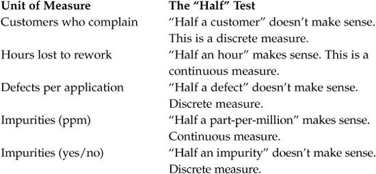
Here’s a quick test for distinguishing between discrete and continuous measures. Think about the “unit of measure”—the thing being measured—and ask yourself if “half of that thing” makes sense. If the answer is yes, the measure is continuous; if no, you have a discrete measure. For example:
The second confusing issue is that some things that can be measured on a continuous scale are sometimes converted into discrete measures. For example, delivery times can be measured as “on time” or “late” (discrete categories) rather than in days, hours, minutes, and seconds (continuous data). On many automobile dashboards, oil pressure gauges showing continuous data have been replaced by warning lights that tell you when pressure is too low, versus OK. Figure 9-1 provides some examples of discrete and continuous data, and how continuous data can be converted to discrete.
The concept of discrete data is important because Six Sigma performance is based on measures of defects, which are usually discrete data, or measures that are converted to discrete items (such as “defects”). Ordinarily, continuous data is preferred because it gives a greater sense of the true variation in the process. Also, if you start with continuous data, you can always convert it to discrete categories by comparing the data against some threshold or criteria—“anything below 50 is a defect” or “any customer with revenues smaller than $500,000 is ‘small.’” In contrast, if you start with discrete data, it’s usually impossible to convert it to continuous data. However, discrete data does have some advantages. Here are some of the reasons in favor of or against discrete data.
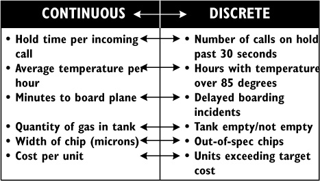
Figure 9-1. Continuous and Discrete Measures of the same variable
The Pros of Discrete Data
♦ Ease of collection. Collecting discrete data is often easier and faster than collecting continuous data because you are measuring whether something meets a standard or not, like a pass/fail test in school, or people who say they liked a movie or didn’t. Many business processes are set up to automatically record discrete data, such as locations (country, state, city, street), customer type (new versus repeat, home versus business user), product number, and product condition (damaged/undamaged).
♦ Ease of interpretation. Intangible factors that would be difficult to measure on a continuous scale can often be converted into discrete measures. Customer satisfaction surveys convert the intangible “customer attitude” into a scale of 1 to 5.
♦ Ease of determining sigma performance level. A sigma calculation tells you how many defects fall within customer requirements—which is an attribute measure (in or out of spec; “OK” vs. “defective”).
The Cons of Discrete Data
♦ A loss of precision. Which would you rather have, a doctor who puts her hand on your forehead and says you’re “feverish” or one who takes your temperature with a thermometer and says your temperature is 102.3 degrees? Continuous data offers more precision than discrete data and, if your time and resources allow it, you’ll want to capture continuous data whenever you can.
♦ The need to collect more data. Interpreting discrete data is basically a question of uncovering patterns in the data categories. And you need a lot of data to accurately judge whether a pattern exists. For example, you should have 50 or 100 data points to use even simple tools like a Pareto chart or some types of bar charts. (In contrast, tools based on continuous data—such as frequency plots and run charts—can often be interpreted with far fewer data points.) The need for more data will stretch out your data collection chores. And the closer your process is to Six Sigma—as you approach as few as 50-60 defects per million opportunities to have something go wrong—you’ll have to collect lots of data just to catch the defects.
♦ Increased likelihood of missing important information. Because of its “either/or” nature, discrete data can hide important detailed information about a service or product.
In short, whenever possible, start with continuous data if time and your budget allows.
Measurement Concept #3: Measure for a Reason
Ever notice how much useless data gets collected at work? It’s probably because the computer has made it easy to collect tons of numbers, however trivial. But don’t let your team get sucked into that quagmire. Unless there’s a clear reason to collect data—a key variable you want to track—don’t bother. There are basically two reasons for collecting data:
1. Measuring efficiency and/or effectiveness
♦ Looking at measures in terms of efficiency and effectiveness keeps your team focused on who will benefit from your improvement efforts: your organization, your customers, or (we hope) both.
♦ Efficiency measures focus on the volume and cost of resources consumed in your processes, and on the improvements you’ve made inside the process resulting in lower costs, less time, fewer materials and staff, etc. Your own organization benefits directly from such reductions, but they will benefit your external customers only if you pass the savings along in some form.
♦ Effectiveness measures reveal what your product or service looks like to the customer. How closely have you met or exceeded their requirements? What defects were delivered to them?
2. Discovering how variables (Xs or causes) upstream in the process affect the outputs (Ys or effects) delivered to the process customer.
♦ This can be described as looking at the relationship between “Predictors” and “Results” (or “leading indicators” and “lagging indicators”). It’s typical to start by measuring outputs or results delivered to customers—be it “good” or “defective.” In the course of your project, you’ll then work your way back into the process to discover measures that predict certain outcomes. For example, a measure of internal cycle time can be a predictor of decreased customer satisfaction if the cycle time means we’ll deliver our product late to the customer.
Being clear about what you want to accomplish with data is the first step in making sure you will be measuring for the right reasons. In choosing measures for your Six Sigma project, make sure you have not focused only on output measures, but have a balance between output and process measures, predictor and results measures. Teams (and their Champions) are tempted to boost efficiency (with its quick bottom-line impact) by streamlining internal processes while forgetting the long-term impact of such measures and changes on the customer.
Measurement Concept #4: A Process for Measurement
Remember the old carpenter’s saying, “Measure twice; cut once”? It should remind us of the importance of getting our measures right the first time. There is nothing more tedious and frustrating than having to collect data a second time because it wasn’t done right the first time. Treating data collection as a process that can be defined, documented, studied, and improved is the best way to make sure you only have to “cut once.” A detailed process is described below.
Two Components of Measure
The guidelines for data collection given above have been incorporated into the two procedures that comprise the Measure stage of DMAIC:
A. Plan and measure performance against customer requirements.
B. Develop baseline defect measures and identify improvement opportunities.
A. Plan and Measure Performance Against Customer Requirements
The following five-step measurement collection plan can help you avoid the most common problems with data collection:
Step A1. Select what to measure.
Step A2. Develop operational definitions.
Step A3. Identify data sources.

Use the Measurement Planning Worksheet in Chapter 10, p. 163, to document your team’s data collection decisions.
Step A4. Prepare a data collection and sampling plan.
Step A5. Implement and refine the measurement process.
Each of these steps is described in more detail below.
Step A1. Select What to Measure
In the Define stage, your team identified the primary problem your DMAIC project will tackle, along with critical customer requirements. Here, start by measuring to validate or refine your understanding of the size and frequency of the problem, along with how well you are meeting the customer requirements (these may be one and the same). In most cases these initial measures will amount to counting the defects that show up in your process’s outputs. Your team will also want to measure the performance of those process steps that seem to contribute most to the output defects (the suspected Xs). In general, pay attention to two areas in selecting measures: what’s valuable for analyzing the problem and what’s feasible to collect. Figure 9-2 shows some criteria for selecting measures.
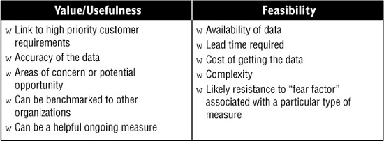
Figure 9-2. Criteria for useful measures
What key questions do you need to answer? What data will provide the answers? What output or Service requirements will best gauge performance against customer needs? What upstream variables in the process will predict problems downstream in the process? How will we display/analyze the data?
Since this is a DMAIC project, one set of data you gather should focus on defects, because you’ll need that data for Step B, in which you refine your process baseline measure—often accompanied by determining baseline sigma levels.
Using the CTQ Tree to Identify Measures
Another approach to identifying measures that relate to customer requirements is called the CTQ Tree. This diagram is like a tree chart except here the focus is on defining measures that are “critical to quality.” Figure 9-3, for example, shows where the team was interested in measuring “timely resolution of service disruptions.” They decided that the measure had two broad components (disruptions fixed per day, and time to restore service), then identified specific, easily measurable data they could collect that would allow them to measure those broad components.

Identify Potentially Related Factors (Stratification)
Imagine that you are collecting complaint data about a product sold nationwide by your company. Now imagine you have that data in hand. What are some questions you’d like that data to answer? For example …
♦ Are there differences by state or region?
♦ Are there differences by demographic factors such as gender, age, or income level?
♦ Are there differences by month of purchase?
All of these questions represent different ways you will want to “slice and dice” your data once you have it in hand. In Six Sigma terms, they are discrete categories (e.g., state, gender, month) that you will use to stratify the data.
Why is this important? Stratification of information can give you clues about where to look for the causes of problems. For example, you might discover that customers in the southwest complain twice as often as those in other parts of the country. That would raise a host of questions for your team: what is it about people in the southwest and how they obtain or use your product that is different from everyone else?
Here’s another example. In one recent nationwide product recall, the cause of the problem wasn’t uncovered until the investigators stratified their data first by product type, then by product size, then by manufacturing plant, and finally by product age at time of failure. Just having data on the number of products that failed couldn’t lead to a solution; this company needed all of that stratification information—product type, size, manufacturing plant, and product age—to dig out the root cause.
Now here’s the key lesson: You can’t stratify data unless you gather the stratification information at the same time as you gather the data. So you need to think about what stratification data you are interested in beforehand, and build those questions into your data collection plan.
There are endless ways to stratify a set of data: knowing which ways will be most useful to your team is five parts experience and five parts guesswork. You’ll find some instructions in Chapter 10 to help you get started.
See Stratification Instructions on p. 165.
Measurement Assessment
A third approach to identifying data that may be useful to your team combines the concepts of a CTQ Tree and stratification. It’s called the Measurement Assessment Tree (see Figure 9-4).
This tree started with an important output for the Six Sigma Pizza Company: number of late deliveries. The metrics—such as “# late by region”—can be directly linked back to the key defect (number of late deliveries) and to important questions about that defect (“what trends or patterns do we see?”).
See the Measurement Assessment Instructions on p. 166. Document your decisions on your Measurement Planning Worksheet, p. 163.
This kind of Measurement Assessment Tree helps your team keep a clear connection between what you’re trying to accomplish and what data will help you get there. By linking the various levels of detail in defining a measure, you can avoid measuring the wrong things and improve the odds of measuring the right things correctly.
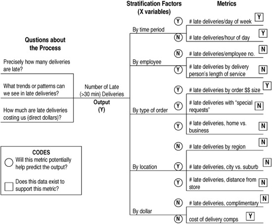
Figure 9-4. Measurement Assessment Tree
Before moving on…
At the end of Measure Step A1: Select What to Measure, you should have:
![]() At least one target measure linked to the project problem and goal—often called the “project Y.”
At least one target measure linked to the project problem and goal—often called the “project Y.”
![]() Potentially one or more target measures of predictors or Xs in the process or inputs that you suspect may help you find or narrow the causes of the problem.
Potentially one or more target measures of predictors or Xs in the process or inputs that you suspect may help you find or narrow the causes of the problem.
![]() An idea of where you’ll gather the data and a fair degree of certainty that the data is available and feasible to be collected (to be refined in coming steps).
An idea of where you’ll gather the data and a fair degree of certainty that the data is available and feasible to be collected (to be refined in coming steps).

Step A2. Develop Operational Definitions
Saying that your team will count the number of defects in a product or service is easy. But what exactly do you mean by “defect,” “product,” and “service”? Without having precise definitions for the things you’re trying to measure, different people will count different things in different ways. To avoid this confusion, you need to have operational definitions:
Operational definition: a clear, understandable description of what’s to be observed and measured, such that different people taking or interpreting the data will do so consistently.
In a recent example of a failure to have such a clear definition, recall the Mars Polar Orbiter that crashed onto the planet surface because one group of engineers had written procedures in English units (pound-seconds) and the computer interpreted the data in metric units (newton-seconds). Or think back to the Florida ballot recounts in the presidential election of 2000: how consistently do you think people interpreted a “pregnant chad”?
The purpose of your operational definition is to translate what you want to know into something you can observe and measure. (As noted, nothing can be measured until it can be observed.)
You’ll find instructions for writing an operational definition in Chapter 10. To make sure your operational definition is airtight, factor in …
♦ Different ways people interpret the same words.
♦ The ability to stay focused on what needs to be observed and/or measured.
♦ Changes or situations that might emerge that require special interpretation.
♦ Events or observations that can fit under more than one grouping or that might be interpreted/measured several ways.
See the Operational Definition Worksheet on p. 169. Document your decisions on your Measurement Planning Worksheet, p. 163.
Step A3. Identify Data Sources
There are two main sources of data available for the team:
1. Data that is already being collected in your organization and has been around for some time (usually called “historical” data).
2. New data your team collects now.
At the end of Measure Step A2: Develop Operational Definitions, you should have:
![]() A clear, detailed, and unambiguous description of what’s being measured.
A clear, detailed, and unambiguous description of what’s being measured.
![]() Guidelines for data collectors on how to interpret routine and/or unusual instances or items.
Guidelines for data collectors on how to interpret routine and/or unusual instances or items.
![]() An initial plan for collecting the data (when and how)—still to be finalized in coming steps.
An initial plan for collecting the data (when and how)—still to be finalized in coming steps.

Historical data can be handy, when you have it—it requires fewer resources to gather, it’s often computerized, and you can start using it right away. But be warned: existing data may not be suitable if…
♦ It was originally collected for reasons other than improving a process or detecting defects.
♦ It was collected using different definitions and methods than what your team has developed.
♦ The data is structured in a way that makes it hard to apply to your needs. For example, key “stratification factors” may not be present. Or the database may not have the capability to sort the specific data you want.
To see if historical data will meet your needs, compare your new operational definition with whatever definition was used at the time the old data was collected. You may be able to adjust your operational definition to fit what’s in the data—as long as it still works in giving the answers you need. Checking the existing data will require a little research, but it’ll be worth it (for example, to make sure that what the shipping department counted as “late deliveries” is the same thing that your customers who take deliveries count as “late”).
Step A4. Prepare a Data Collection and Sampling Plan
A data collection and sampling plan covers three main issues:
A4.1: Identify or confirm the stratification factors.
A4.2: Develop a sampling scheme.
A4.3: Create data collection forms.
At the end of Measure Step A3: Identify Data Sources, you should have:
![]() A decision on whether you need to gather new data or can rely on existing or historical data.
A decision on whether you need to gather new data or can rely on existing or historical data.
![]() Validation of the ability to access and sort existing data (if that’s the choice).
Validation of the ability to access and sort existing data (if that’s the choice).

Step A4.1: Identify or Confirm the Stratification Factors
Stratification was introduced earlier in this chapter (pp. 135-136) as a technique for gathering information that can help in tracking down clues to root causes. Your decisions about what stratification questions you’re interested in will affect how you gather and sample data. For example, if you want to compare survey results between the Central Rockies and West Coast regions, you need to make sure that you’ve collected enough information from both regions to draw valid conclusions.
If you have already identified stratification information, you just need to confirm those decisions here. If not, make sure that you don’t want to gather such information before proceeding with your sampling strategy.
Step A4.2: Develop a Sampling Scheme
Deciding how you will collect sample data involves logical thinking about how your potential data sources are structured. In the example below, pay attention to the italicized words—they reflect key concepts in sampling.
A Brief Sampling Saga: HomeHealth Products
HomeHealth Products distributes medical supplies and equipment to healthcare resellers throughout the United States. As part of its implementation of Six Sigma in its eight regional centers, HHP (as its employees call it) has taken on a chronic problem that has been an issue for the company and its reseller clients for years: the variance between what appears on the bills of lading HHP sends with its shipments and the data for the same materials that appears in the internal logistics computer system. The differences between the numbers lead to billing and inventory problems that a recent survey of HHP’s top customers described as “unprofessional,” “intolerable,” and “likely to lead to non-renewal of existing contracts.”
“The Voice of the Customer is talking loud and clear,” said Bill Wrigley, Directing Manager of the Eastern Regional Center, to Ed Magos, who managed several of the processes under review, and Jane Medawar, a Six Sigma Black Belt who had been leading a team working on the problem for the last few weeks. The team had finished the “Define” stage and was about to get into “Measure.”
“Just measuring the problem is a bear,” said Ed Magos. “We take in nearly 800 shipments at the warehouse every day, and send out 1000 shipments of our own to the resellers every day.”
“Obviously you can’t check them all,” said Bill Wrigley. “You’ll have to do some sampling.”
“Our team is putting together its data collection plan now,” said Jane Medawar, “and sampling is part of the plan. But we’re worried about bias getting in the way of a good sample.”
“I don’t know about bias,” said Bill. “What you need is a good sampling plan.”
Ed suggested that the team might sample the shipments by having the packers and shippers collect data when they’re not so busy, like on the swing shift.
“We talked about that,” said Jane, “but the data will be biased if we just collect data when it’s convenient for us.”
“Well,” said Bill, “I’m no statistician, but why not have the shippers pick out the shipments they think are most representative of a normal day? After all, they know more about shipping than the rest of us.”
“I agree,” Jane replied, “and we’ve got three people from shipping on the team. But when I asked them which shipments they judged most representative of a normal day, they all had different ideas and disagreed with one another.”
Bill seemed a little frustrated as he spoke next.
“So how are you going to sample the shipments, Jane?”
“We’ve pretty much decided to take a systematic approach. We’ll take some measures on every tenth or twentieth shipment. We haven’t figured out yet exactly how often or how many we’ll look at. That’s coming up at the next meeting. Once we’ve figured that out we’ll have more confidence in our data collection plan.”
“I know you’re the Black Belt,” said Ed, who was the project Champion and Jane’s boss, “but isn’t it always better to take a random sample?”
Jane smiled. The team had been through all this at their last meeting.
“In theory, yes. Random is best, but in practice it’s not all that easy. Systematic sampling will help us spot any patterns in the data from the shipments. Of course, we’ll have to make sure our systematic sample isn’t based on some hidden pattern itself, like always picking samples right after break or something like that.”
“Well, Jane,” said Bill, “it sounds like you’ve thought it through. Good luck. If we can get some improvement on this problem it’ll save us a ton of rework, and maybe just two or three key customers.”
Jane’s team still had some work to do on the sampling plan….
In data collection, sampling means measuring some of the items in a group or process to represent them all. If you’re processing large numbers of things, you can’t count every item. But if you only pick out a few, how can you be confident they represent the whole group?
If you’ve taken a statistics course, you know how big a part sampling plays. Most college statistics courses focus on “population statistics,” which assume that we have a large, standing pool of water (or data), and that if you take a dipperful at any point, it will represent all the rest of the water (or data).
In the business world, however, there isn’t much standing water, so your team may be more interested in “process statistics,” or taking a sample from a running stream of water that may be changing minute by minute, depending on what you’re measuring. Table 9-1 shows examples of both types.
Whether you’re sampling a whole population of data or a moving process, you still need a valid sample—one that actually represents the whole. The next few pages cover some sampling basics to get you started. If your situation is complex and the results are critical, contact a statistical expert for specific advice.
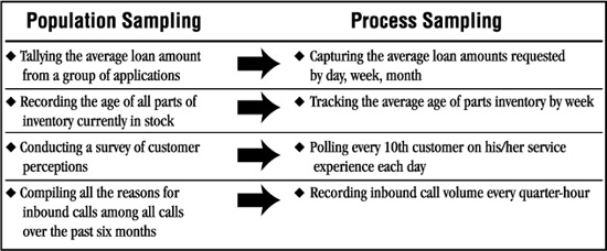
Table 9-1. Examples of Population and Process Sampling on similar items
Sampling Concept #1: Bias
Bias is the difference between the data collected in a sample and the true nature of the entire population or process flow. Bias that goes undetected will influence your interpretation and conclusions about the problem and process. Here are some examples of types of sampling bias:
♦ Convenience sampling: Collecting data simply because it’s easy to collect. Example: collecting data every afternoon 20 minutes before closing time because “things are quiet then,” thus ignoring data when things are busy— which might be very different data.
♦ Judgment sampling: Making educated guesses about which items or people are representative of your process. Example: surveying only those customers who scored high on your last customer satisfaction survey.
Better sampling strategies—better able to avoid bias—include:
♦ Systematic sampling: This is the method we’d recommend for most business processes. By systematic sampling of a process we mean taking data samples at certain intervals (every half-hour or every 20th item). A systematic sample from a population would be to check every 10th item in the database. But beware! Make sure your systematic sampling doesn’t correspond to some hidden pattern that will bias the data. Example: Sampling every 10th insurance claim might mean that you always get claims reviewed by the same clerk on the same computer, while ignoring four other clerks and their computers.
♦ Random sampling: By random we mean that every item in a population or a process has an equal chance to be selected for counting. Selecting data randomly has its own challenges, not least of which are unconscious biases or hidden patterns in the data. Most random sampling is done by assigning computer-generated random numbers to items being surveyed.
♦ Stratified sampling: Suppose your company had a customer base of 10,000 purchasers, and your job is to survey a sample to determine customer satisfaction. Are you equally interested in what all 10,000 customers have to say? The answer is probably “no.” It’s likely more important that you understand the needs and perceptions of your biggest customers or most reliable purchasers than it is that you find out what a onetime customer thinks. (The opposite would be true if you were trying to expand market share; in this case, you might want to understand how you could convert infrequent customers into regular purchasers/users.)
If there are cases like this where there is structure in the population or process flow, you can develop a stratified sampling scheme—either random or systematic. In the customer satisfaction example, that might mean dividing the 10,000 names into, say, four groups: large regular purchasers, small regular purchasers, infrequent but recent purchasers, and lapsed customers. You could then use different schemes to randomly sample from each of these groups, perhaps choosing one out of every five large regular purchases but only a handful of lapsed customers.
See the Sampling Definitions and Worksheets on pp. 170-173.
Attach your sampling plan to your Measurement Planning Worksheet, p. 163.
A stratified sample helps avoid the gaps that can come up if data are collected over a large population where key subgroups of the population are underrepresented.
Sampling Concept #2: Confidence Level or Interval
This is your level of confidence that the data you sample actually represents the entire population or process under study, provided the sample was gathered randomly. In the business world, a confidence level of 95% is standard. It means that you have five chances out of 100 of drawing the wrong conclusion from your data.
There’s a “Catch 22” to developing a good sampling plan: You already have to know something about the data you’re collecting before you collect it. As a result, your first measures won’t be as reliable as you’d like because they’re based on educated “guesstimates.” The longer you take measures, however, the better you’ll know your process and the better your sampling plan will be.
Instructions for Developing a Sampling Plan
The Sampling Worksheets in Chapter 10 will help you develop a sampling scheme appropriate for your project. As a preview, you will need to know whether you are measuring from a process or population; the form itself will walk you through the decisions necessary to determine an appropriate sampling scheme.
If you have trouble making the decisions required to complete the sampling worksheets, contact a statistician familiar with your processes and operations.
Step A4.3: Create Data Collection Forms
Now that you’ve made decisions about what data and stratification information you want to collect and what sample sizes are appropriate, you need to document those decisions on a Data Collection Form. Spreadsheets or checksheets are the workhorses of data collection. While each checksheet will vary depending on the data collected, the following guidelines will help you avoid some common pitfalls in collection forms:
See Checksheet Development Instructions on pp. 175-176.
♦ Keep it simple. If the form is cluttered, hard to read, or confusing, there’s a risk of errors or nonconformance.
♦ Label it well. Make sure there is no question about where data should go on the form.
♦ Include space for date, time, and collector’s name. These obvious details are often omitted, causing headaches later.
♦ Organize the data collection form and compiling sheet (the spreadsheet you’ll use to compile all the data) consistently.
♦ Include key factors to stratify the data.
Common types of checksheets include …
♦ Defect or Cause Checksheet. Used to record types of defects or causes of defects. Examples: reasons for field repair calls, types of operating log discrepancies, causes of late shipments.
♦ Data Sheet. Captures readings, measures or counts. Examples: transmitter power level, number of people in line, temperature readings.
♦ Frequency Plot Checksheet. Records a measure of an item along a scale or continuum. Examples: gross income of loan applicants, cycle time for shipped orders, weight of packages.
♦ Concentration Diagram Checksheet. Shows a picture of an object or document being observed on which collectors mark where defects actually occur. Examples: damage done to rental cars, noting errors on application forms.
♦ Traveler Checksheet. Any checksheet that actually travels through the process along with the product or service being produced. The check-sheet lists the process steps down one column, then has additional columns for documenting process data. Figure 9-5, for example, shows a simple traveler checksheet where the team monitoring how long it took loan applications to complete each step of the process (time information should almost always be collected) and the number of defects found. Some examples of traveler checksheet uses are capturing cycle time data for each step in an engineering change order, noting time or number of people working on a part as it is assembled, tracking rework on an insurance claim form.
Before moving on…
At the end of Measure Step A4: Prepare a Collection and Sampling Plan, you should have:
![]() A list of stratification factors that are potentially important to your project.
A list of stratification factors that are potentially important to your project.
![]() A completed sampling plan.
A completed sampling plan.
![]() Data collection forms.
Data collection forms.

Step A5. Implement and Refine the Measurement Process
There are five steps in implementing and refining the measurement process:
A5.1: Review and finalize your data collection plans.
A5.2: Prepare the workplace.
A5.3: Test your data collection procedures.
A5.4: Collect the data.
A5.5: Monitor accuracy and refine procedures as appropriate.
Step A5.1: Review and Finalize Your Data Collection Plans
Complete your Measurement Planning Worksheet. Determine how you will assess the accuracy and reliability of the measurements. Measurement practices and measuring devices themselves are subject to variation. No matter how well you train people, it’s likely they will vary slightly in how they collect data; and instruments are known to degrade in precision over time. Six Sigma teams need to take this variation into account. Especially if you repeat measurements over time, you’ll have to keep an eye on several factors:
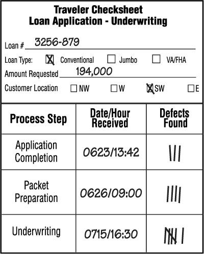
Figure 9-5. Example of a Traveler Checksheet (one that is attached to a document or product as it goes through a process)
♦ Accuracy: How precise is the measurement: hours, minutes, seconds, millimeters, two decimal places?
♦ Repeatability: If the same person measures the same unit with the same measuring device, will they repeat the same results every time they do it? How much variation is there between measurements?
♦ Reproducibility: If two or more people or devices measure the same thing, will they produce the same results? What is the variation?
♦ Stability: How much do accuracy, repeatability, and reproducibility change over time? Do we get the same variation in measures that we did a week ago? A month ago?
Part of your plan should include procedures to ensure that your data continue to be valid throughout the data collection process.
Step A5.2: Prepare the Workplace
Explain clearly why you’re gathering the data. Describe what you plan to do with the data—including your plan to share the results with the data collectors, keeping identities confidential, and the like.
Step A5.3: Test Your Data Collection Procedures
Be careful whom you choose as data collectors; avoid making data collection a reward or punishment. When you collect new data using your operational definitions, it’s best to experiment a little at first, gathering data manually from people in the process. (There’s a temptation for many teams to create an elaborate IT computerized system right away. But you’ll learn more and be able to better refine your system if you do some initial data collection with pencil and paper or your own laptop.)
In manufacturing, accuracy of gathering continuous data is ensured through the calibration of measuring devices. With discrete measures—either in service or manufacturing—one method of testing repeatability and reproducibility is to have one or more people count the number of defects on documents that have been carefully inspected before by an expert who has counted the precise type and number of defects. The results of the counters are then compared to those of the expert, and the variation measured.
Step A5.4: Collect the Data
Implement your plans. Remember that part of your plan includes the “sample size,” that is, the number of data points you have to collect. Your data collection should stop when you’ve reached the appropriate sample size, unless there were problems with some of that data. Do not continue to collect data unless there are plans to make it a standard part of the process.
Step A5.5: Monitor Accuracy and Refine Procedures as Appropriate
Throughout the data collection, be sure to monitor both the procedures and devices (if any) used to collect the data.
At the end of Measure Step A5: Implement and Refine the Measurement Process, you should have data in hand that:
![]() Meet your data collection priorities.
Meet your data collection priorities.
![]() Were sampled according to your plan.
Were sampled according to your plan.
![]() Reflect accurate, repeatable, reproducible, and reliable measurement practices.
Reflect accurate, repeatable, reproducible, and reliable measurement practices.

B. Develop Baseline Defect Measures and Identify Improvement Opportunities
The measurement and sampling methods described above are important any time your team is gathering data. At this point on the road to Six Sigma, however, your team needs to baseline the performance of the process under investigation—determine how the process and product/service are working today, before you start making changes. You’ll gauge improvements against this baseline later.
Instructions for completing this process appear later in this chapter (starting on p. 150). Before you begin, however, you need to understand what it means to measure the sigma performance of a process. Typically, people start by looking at measures for process outputs, then work their way upstream to look for measures of how the process itself is performing.
See the Sigma Calculation Worksheet on p. 178 and the Sigma Conversion
Output Performance Measures
Six Sigma performance measures are most often based on defects produced by the process. There are several advantages to basing measurements on defects, including:
♦ Simplicity: Anyone who can understand “good” and “bad” can understand “good” and “defective.”
♦ Consistency: Defect measures apply to any process for which there are customer requirements, whether we are measuring manufacturing or services, using continuous or discrete data.
♦ Comparability: Motorola and other Six Sigma companies use defects to track and compare performance in very different areas across the business. The same measure allows teams to measure their improvements over the course of their projects and beyond.
A drawback of looking only at good versus defective is that defect counts may hide important variations in the numbers—especially with continuous data like time. The aim here is not to burden you with lots of qualifiers, but to give you a good foundation for measuring what’s actually going on in your processes and determine the causes of problems and unwanted variation.
Here are three steps that will help translate the concepts about sigma capability into concrete numbers useful to your team:
Step B1. Calculate baseline sigma levels for the process as a whole.
Step B2. Calculate final and first-pass yield.
Step B3. Determine the “Cost of Poor Quality.”
Step B1. Calculate Baseline Sigma Levels for the Process as a Whole
Calculating baseline sigma for process, product, or service is a simple four-step process. You’ll need to do some simple math and consult one conversion table. A worksheet for the sigma calculation is in Chapter 10 (p. 178); you’ll need to be familiar with the following terms and concepts in order to complete that worksheet.
The Key Definitions: Units, Defects, and Defect Opportunities
The Six Sigma team needs to understand a few key terms both to collect and analyze data used to determine the capability of its process:
♦ Unit: An item being processed, or the final product or service being delivered either to internal customers (other employees working for the same company as the team) or external customers (the paying customers). Examples: a car, a mortgage loan, a computer platform, a medical diagnosis, a hotel stay, or a credit card invoice.
♦ Defect: Any failure to meet a customer requirement or performance standard. Examples: a poor paint job, a delay in closing a mortgage loan, the wrong prescription, a lost reservation, or a statement error.
♦ Defect Opportunity: A chance that a product or service might fail to meet a customer requirement or performance standard.
Of these terms, defect opportunity is the trickiest to implement and most critical for calculating a reliable sigma capability figure. The defect opportunity component of a Six Sigma calculation is what enables us to compare processes of different complexity. As a simple example, consider two people who are both making phone calls. Rita is calling local numbers and only has to dial seven numbers per customer. Gordie has a long-distance calling card (with a PIN) and is making international calls. He often has to dial two or three times as many numbers as Rita just to complete one call.
The data show that both Rita and Gordie have one wrong number for each 100 calls they make. But is that an accurate comparison? In Six Sigma terms, Gordie’s process has many more “opportunities” for making a mistake when dialing a phone number because he has to dial so many more numbers. Looked at another way, Rita is making one mistake in every 700 digits she dials; Gordie is making one mistake in every 1,400 to 2,500 numbers he dials. So whose process has fewer defects?
In a world where Murphy’s Law is widely understood, you might think that there are thousands and thousands of chances for things to go wrong. In reality, that is seldom the case, though in some very complex systems it could actually be more than that.
Two guidelines prevent the use of defect opportunities from becoming a nightmare:
♦ First, you need to focus on defects that are important to the customer. Consider a bank that regularly makes two kinds of mistakes: (1) mailing out monthly statements a day late, and (2) entering interest payments a day late. Which of these defects do you think is really important to most customers? So we link opportunities in most cases to a CTQ Tree (see p. 135).
♦ Second, defect opportunities reflect the number of places where something in a process can go wrong, not all the ways it can go wrong. So, for example, you would define “wrong address” as one opportunity for a defect on a database record rather than describing all the ways in which that address could be wrong (incorrect street number, street name, wrong ZIP code, etc.). The more opportunities we add, the more things look fishy—because more opportunities mean better-looking performance.
Here’s an example. Any time a clerk types a form, application, report, etc., every key stroke could theoretically be counted as a defect opportunity. However, that is not only impractical, but it would also clump important defects along with lots of unimportant defects. In many cases, reports and forms like applications have standard templates that are filled automatically with identical text. The key in these kinds of situations would be to focus on defects that are important to and would be noticed by either the customer or the next step in your process.
For example, here’s a list of 16 opportunities for defects on a generic invoice:
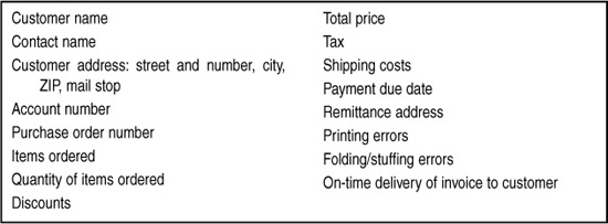
Your team might feel that list of defect opportunities is still too long: it might be difficult to measure all these defects, and some of them are less important to customers than others. So another option would be to combine the various individual defects into four categories of opportunities, as follows:
1. Customer data (name, billing address, purchase order number)
2. Order information (items, quantity, shipping address)
3. Pricing (unit price, tax, discounts)
4. Production (print quality, mailers included)
The shorter list of categories still reflects the complexity of the invoice and the importance of the information to the customer, but makes it easier to capture the data. In fact, as long as the team is consistent in the counting of defect opportunities, and your reasoning is sound, you can make a case for either 16 or four as the number to use.
For the sake of convenience and practicality, it makes sense to define defect opportunities in a way that keeps the number fairly low. On the other hand, you can artificially inflate your sigma level by making the number high.
Consider this example. You know your order entry process generally results in three typos per form. If, like the invoice example above, you define four defect opportunities on the form, you’re looking at a defect rate of three out of four— and a sigma level near zero! On the other hand, if you count every key stroke as an “opportunity,” you’re looking at something closer to three defects per 200 opportunities, and a sigma level of about 3.7. Which sigma level would you rather report? Which would you rather have?
Tips for Defining Defect Opportunities
Here are a few more tips on using defect opportunities for your products and services:
♦ Focus on “routine” defects: Defects that are extremely rare shouldn’t be considered as opportunities.
♦ Group closely related defects into one opportunity category: This will simplify the work of gathering data.
♦ Be consistent: As Six Sigma spreads throughout your company, you should consider using standard definitions of defect opportunities across the board.
♦ Change definitions only when necessary: The team will use the number of defect opportunities to calculate a baseline sigma measure at the beginning of the project, and then compare that number to the improved sigma number near the end of the project. So stick with the same defect opportunities throughout the project.
Example of a Six Sigma Calculation
Figure 9-6 shows some examples of Six Sigma levels calculated using the worksheet in Chapter 10 and applying the definitions given above (DPMO = defects per million opportunities).
If the data is accurate and the defect opportunities are consistently applied, the microchip manufacturing process is functioning most effectively and the advertising contract process is worst. Another way to say this is that the manufacturing process does a better job of meeting customer requirements and has the least amount of rework to fix defects.
Assuming that your team did a good job identifying customer requirements and carrying out your data collection plan, you should have the correct data you need to calculate the baseline sigma number for your output measures. Outputs, or Ys, you’ll recall, are the products and services you deliver to external, paying customers or to other internal customers within your own organization.
See Sigma Calculation Worksheet on p. 178.
Once your team has completed the sigma level, keep that number handy; you’ll want to recalculate the sigma level after you’ve made improvements and compare it to this original baseline.

Figure 9-6. Sample Six Sigma calculation
Before moving on…
At the end of Measure Step B1: Calculate Baseline Sigma, you should have:
![]() Defined units, defects, and defect opportunities for your process.
Defined units, defects, and defect opportunities for your process.
![]() Calculated baseline sigma.
Calculated baseline sigma.

Step B2. Calculate Final and First-Pass Yield
The previous discussion has focused on determining sigma capability at the end of a process, based on the results (output). That’s fine if all you want to do is focus on the capability of our process to meet external customer requirements. But a low output sigma number obviously means that the “innards” of our process are not working very well.
Imagine a process in either services or manufacturing. As Figure 9-7 shows, data collected at the output of the process showed a final yield of .985 (98.5%) and a sigma level of 3.7. Of the original 1,500 units (orders, parts, etc.) that entered the process, only 1,477 emerged “defect-free” as outputs at the end of the process.
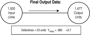
Figure 9-7. Overall process sigma based on final output
Now look inside this process. It has three major subprocesses, each of which operates with a yield of good product in the upper 90th percentile range. The company catches and reworks defects, and over the course of the whole process, 89 units have to be reworked before delivery to the paying customer (see Figure 9-8). So of those 1,500 units, only 1,411 remained defect-free throughout the whole process; the other 89 needed some rework. (Apparently, some of that rework was beneficial since customers received 1,477 “defect-free” units!)
The comparison of these two types of yield introduces two important Six Sigma terms:
♦ The figure of 1,477 is called the final yield, because it measures how many units finally came through the process without defects.
♦ The figure of 1,411 is called first-pass yield, because it measures the number of units that made it through the first time without needed rework.
As Figure 9-8 shows, once you take into account all the rework that has to take place, the percentage of “defect-free” items falls to 94%.
The comparison of these two measures of yield points out the difference between focusing only on outputs (final yield) versus looking at what happens inside a process (first-pass yield). Yields that are measured only as outputs hide defects and the costs associated with them. In some service businesses the costs associated with a low first-pass yield can reach 20% or more of total sales revenues.
See Proportion Defective and Yield Calculation Instructions on p. 180.
Your Six Sigma team will have to decide whether to focus on output results only, or look at the various components of a process. Looking at internal subprocesses can help you target your improvement efforts. Figure 9-9 shows the first-pass yield for the three component steps in our imaginary process. As you can see, the third step has the lowest yield, and therefore might be ripest for improvement.
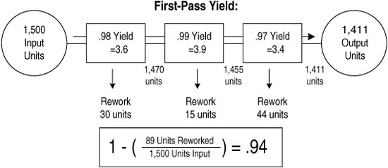
Figure 9-8. Calculating first-pass yield
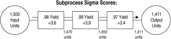
Figure 9-9. Sigma calculation based on subprocess capability
If you choose to take the latter approach, remember that just as the outputs for the entire process are measured against the requirements of the external customer, the outputs of key internal process steps are measured against the requirements of the internal customer. These internal customers are other people who work for the same company as you and are your customer in the sense that they are closer to the external customer and their requirements help determine what you do in your own process.
Step B3. Measuring the “Cost of Poor Quality”
Neither defect counts nor sigma measures directly capture the costs associated with poor quality. Two different processes may both measure in at 3.5 sigma, meaning that their capabilities are roughly equal, but the dollars lost due to the defects in the processes can be very different. For example, a malpractice suit costs more than retaking an x-ray picture.
Before moving on…
At the end of Measure Step B2: Calculate Final and First-Pass Yield, you should have:
![]() Calculation of final yield.
Calculation of final yield.
![]() Calculation of first-pass yield.
Calculation of first-pass yield.

For this reason, you should measure the Cost of Poor Quality (COPQ) as soon as you have collected defect data. This means translating problems or defects into dollar costs per defect—including labor and materials costs for rework. Measuring COPQ can help get support for improvements the team creates, and gets the attention of managers who may find the language of sigma measures a little strange at first, but who recognize the value of increased revenues or savings when they see them.
See Cost of Poor Quality instructions on p. 181 and Measure Checklist on p. 183.
Before moving on…
At the end of Measure Step B3: Measuring the “Cost of Poor Quality,” you should have:
![]() Identified labor and materials costs for rework.
Identified labor and materials costs for rework.
![]() Translated defects into dollar costs per defect.
Translated defects into dollar costs per defect.

Getting Ready for Analyze
By the end of the Measure phase of DMAIC, your team has data that will inform your improvement decisions, and a baseline against which your progress will be measured. The measurement of sigma, yield, defects, and cost of poor quality lay the foundation for what every Six Sigma company needs: a reliable and thorough system of measuring both processes and outputs for customers.
Three of the last steps for completing Measure are the same as for Define, but there is an additional first step:
1. Revisit your problem statement.
2. Create a plan for Analyze.
3. Update your Project Storyboard.
4. Prepare for your tollgate review by your Sponsor or Leadership Council.
5. Celebrate.
1. Revisit Your Problem Statement
Even before completing a thorough analysis of your data, it’s likely your team has learned more about the initial problem that sparked this project. Refine the Problem Statement as appropriate, perhaps by providing more specificity about what the problem is or how it impacts the organization.
2. Create a Plan for Analyze
By the end of Define, you know how much data you’ve collected, and probably have a gut feeling for how easy or difficult it’s going to be to analyze that data. Think ahead and create a plan for the Analyze work. As before, if you are a novice team leader, you can keep the plan simple:
♦ Assign responsibilities within the team for completing the data analysis (often, the initial work is completed by a subteam, who presents the results to the team for discussion).
♦ Set or confirm a target date for completion of the data analysis.
♦ Have your team meetings scheduled.
♦ If most people on the team are new to data analysis, you may want to check with your Coach/Black Belt or a Master Black Belt to arrange for extra support.
3. Update Your Storyboard
The Measure section of your storyboard should display your data collection plan, a few data collection forms, and a revised Problem Statement (if you changed it). You might also consider including a process diagram that highlights problem areas. There may be measures of the sigma level of the process here, as well as rough estimates of the cost of defects and their rework in the process.
4. Prepare for the Tollgate Review
Before you prepare for the Measure Tollgate Review, do a debrief with the team on what happened last time:
♦ What did you do well as a team in the Define review?
♦ What could have been done better?
♦ What did the reviewers (your customers!) say?
♦ Which of the support materials (slides, overheads, handouts, flipcharts, etc.) worked and which didn’t?
See the Measure Tollgate Preparation Worksheet on p. 185.
♦ How did you do on time? If it was too long, what could you do this time to make sure you keep it brief? If it was too short, do you need to add in more detail? Speak more slowly?
After this general review, start your preparation for the Measure Tollgate Review. The main difference between this review and that for Define is that you need to clearly link the work you did here with what came before and what you expect to come after.
Review the tips given in the Measure Tollgate Instructions (p. 182).
5. Celebrate
Once again, take time to celebrate the work and progress on your Six Sigma projects. Be sure to point out particular challenges that the team handled well in its Measure work; for example:
♦ Coming up with innovative data collection ideas.
♦ People maintaining their level of commitment, carrying through on assignments.
♦ Finally having a sigma level for the process (which might be the first time an objective measure has been used!).
Once these steps are complete, your team is ready for Analyze.