Calculus
4.1 Differentiation
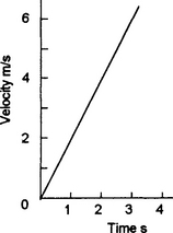
Suppose we have an equation describing how the distance covered in a straight line by a moving object varies with time. We could plot a graph of displacement against time and determine the velocity at some instant as the gradient of the tangent to the curve at that instant. By taking a number of such gradient measurements we could then determine how the velocity varied with time. However, differentiation is a mathematical technique which can be used to determine the rate at which functions change and hence the gradients, this thus enabling the velocity to be obtained from the equation without drawing the graph and tangents. We could also, for example, describe how the deflection of an initially horizontal beam in the y-direction alters with distance along the beam in the x-direction, or how the volume of a gas changes with temperature, or how electric charge at a point in a circuit changes with time (called current), etc. The list of uses is endless!
Limits
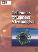
Consider the problem of determining the gradient of a tangent at a point on a graph. It might, for example, be a distance–time graph for a moving object to determine velocity as the rate at which distance is covered or a current–time graph for the current in an electrical circuit in order to determine the rate of change of current with time. Suppose we want to determine the gradient at point A on the curve shown in Figure 4.1. We can select another point B on the curve and join them together and then find the gradient of the line AB. The value of the gradient determined in this way will depend on where we locate the point B. If we let B slide along the curve towards A then the closer B is to A the more the line approximates to the tangent at point A. Thus the line AB1 is a better approximation to the tangent than the line AB. The method we can use to determine the gradient of the tangent at point A is:
1. Take another point B on the same curve and determine the gradient of the line joining A and B.
2. Then move B closer and closer to A. In the limit, as the distance between A and B becomes infinitesimally small, i.e. as AB tends to zero (written as AB → 0), the gradient of the line becomes the gradient of the tangent at A.
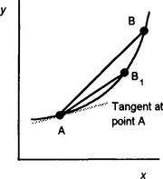
Consider the gradient of the line AB in Figure 4.2:
The gradient is the difference in the value of y between points A and B divided by the difference in the value of x between the points. We can write this difference in the value of x as δx and this difference in the value of y as δy. The δ symbol in front of a quantity means ‘a small bit of it’ or ‘an interval of’. Thus the equation can be written as
An alternative symbol which is often used is Δx, with the Δ symbol being used to indicate that we are referring to a small bit of the quantity x. These forms of notation do not mean that we have δ or Δ multiplying x. The δx or Δx should be considered as a single symbol representing a single quantity.
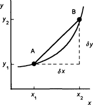
As we move B closer to A then the interval δx is made smaller. The gradient of the line AB then becomes closer to the tangent to the curve at point A (Figure 4.3). Eventually when the difference in x between A and B, i.e. δx, tends to zero then we have the gradient of the tangent at point A. We can write this as:
This reads as: the limiting value of δy/δx as δx tends to a zero value equals dy/dx. A limit is a value to which we get closer and closer as we carry out some operation. Thus dy/dx is the value of the gradient of the tangent to the curve at A. Since the tangent is the instantaneous rate of change of y with x at that point then dy/dx is the instantaneous rate of change of y with respect to x. dy/dx is called the derivative of y with respect to x. The process of determining the derivative for a function is called differentiation. The notation dy/dx should not be considered as d multiplied by y divided by d multiplied by x, but as a single symbol representing the gradient of the tangent and so the rate of change of y with x; if you like, it is a shorthand way of writing ‘the rate of change of y with respect to x’.
For any graph of y = f(x), if A is the point (x, y), i.e. (x, f(x)), and B the point (x + dx, y + δy), i.e. (x + δx, f(x + δx)), then the gradient of the tangent at point P at the limiting value as the δx tends to zero:
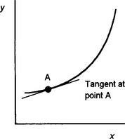
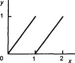
Since we can interpret the derivative as representing the slope of the tangent to a graph of a function at a particular point, this means with a continuous function, i.e. a function which has values of y which smoothly and continuously change as x changes for all values of x, that we have derivatives for all values of x. However, with a discontinuous graph there will be some values of x for which we can have no derivative. For example, with the graph shown in Figure 4.4, there is no derivative for x = 1.
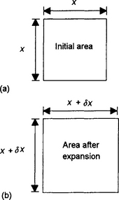
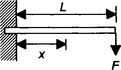
There are situations in engineering where, given an initial condition of some variable, we need to determine its rate of change with respect to some parameter. As an illustration, consider a square flat metal plate of side length x (Figure 4.5(a)). The initial condition we are concerned with is the area A of the plate:
Now suppose the plate is heated and the dimension x changes by an amount δx (which is small compared with the original dimension x but which may have an effect on such things as tolerances in assembly). The plate, which expands equally in all directions, now has sides of length (x + δx) (Figure 4.5(b)). The new area is thus:
If we denote the changes in area as δA, then:
Since dx is very small, then (δx)2 → 0 and in this limiting condition we can write:
We now have an expression which describes how the rate of change of the area with side length depends on the side length. We have determined the derivative.
4.1.1 Derivatives of common functions
The above examples illustrate how, given some initial condition, we can determine the derivative of a function. Rather than always work from first principles in this way, it is useful to work out some general rules we can use. The following illustrates how some commonly used functions can be differentiated.
Derivative of a constant
A graph of a constant, e.g. y = 2, has a gradient of 0. Thus its derivative is zero. Thus for y = c, where c is a constant:
Derivative of xn
If we differentiate from first principles y = x we obtain dy/dx = 1. If we differentiate y = x2, as in the above example and maths in action, we obtain dy/dx = 2x. If we differentiate y = x3 we obtain dy/dx = 3x2. The pattern in these differentiations is that if we have y = xn, then:
This relationship applies for positive, negative and fractional values of n.
Derivatives of trigonometric functions
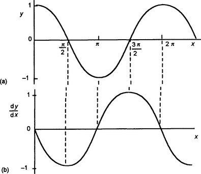
Consider the determination of how the gradients of the graph of y = sin x (Figure 4.6(a)) vary with x. Examination of the graphs shows that:
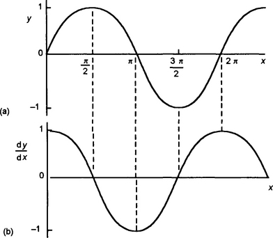
1. As x increases from 0 to π/2 then the gradient, which is positive, gradually decreases to become zero at x = π/2.
2. As x increases from π/2 to π then the gradient, which is now negative, becomes steeper and steeper to reach a maximum value at x = π.
3. As x increases from π to 3 π/2 then the gradient, which is negative, decreases to become zero at x = 3 π/2.
4. As x increases from 3 π/2 to 2 π the gradient, which is now positive again, increases to become a maximum at x = 2 π.
Figure 4.6(b) shows the result that is obtained by plotting the gradients against x; it is a cosine curve. Thus, the derivative of y = sin x is:
We can prove that the above is the case as follows. For the function f(x) = sin x, we have f(x + δx) − f(x) = sin(x + δx) − sin x. Using equation [28] from chapter 1 for the sum of two angles, sin (x + δx) = sin x cos δx + cos x sin δx. As δx tends to 0 then cos δx tends to 1 and sin δx to δx. Thus, the derivative can be written as:
If we had considered the function sin ax then we would have obtained:
The derivatives of tan ax, cosec ax, sec ax and cot ax can be derived using the quotient rule (see later in this chapter) as:
The derivatives of sin (ax + b), cos (ax + b), etc. can be derived by using the chain rule (see later in this chapter) as:
In a similar manner we can consider y = cos x (Figure 4.7(a)) and the gradients at various points along the graph.
1. Between x = 0 and x = π/2 the gradient, which is negative, becomes steeper and steeper and reaches a maximum value at x = π/2.
2. Between x = π/2 and x = π the gradient, which is negative decreases until it becomes zero at x = π.
3. Between x = π and x = 3π/2 the gradient, which is positive, increases until it becomes a maximum at x = 3π/2.
4. Between x = 3π/2 and x = 2π the gradient, which is positive, decreases to become zero at x = 2π.
Figure 4.7(b) shows how the gradient varies with x. The result is an inverted sine graph. Thus, for y = cos x:
If we had considered y = cos ax, where a is a constant, then we would have obtained for the derivative:
We can prove that the above is the case in a similar way to that used for the sine.
Consider a sinusoidal current i = Im sin ωt passing through a pure inductance. A pure inductance is one which has only inductance and no resistance or capacitance. With an inductance a changing current produces a back e.m.f. of −L × the rate of change of current, i.e. L di/dt, where L is the inductance. The applied e.m.f. must overcome this back e.m.f. for a current to flow. Thus the voltage across the inductance is L di/dt. Hence:
Since cos ωt = sin (ωt + 90°), the current and the voltage are out of phase with the voltage leading the current by 90°.
Consider a circuit having just pure capacitance with a sinusoidal voltage v = Vm sin ωt being applied across it. A pure capacitance is one which has only capacitance and no resistance or inductance. The charge q on the plates of a capacitor is related to the voltage v by q = Cv. Thus, since current is the rate of movement of charge dq/dt.

i.e. i = C dv/dt. Since current is the rate of change of charge q:
Since cos ωt = sin (ωt + 90°), the current and the voltage are out of phase, the current leading the voltage by 90°.
Derivatives of exponential functions
Consider the exponential equation y = ex and a small increase in x of δx. The corresponding increase in the value of y is δy where:
Thus:
If we let δx = 0.01 then (e0.01 − 1)/0.01 = 1.005. If we take yet smaller values of dx then in the limit this has the value 1. Thus:
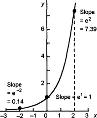
The derivative of ex is ex. Thus the gradient of the graph of y = ex at a point is equal to the value of y at that point (Figure 4.8). For example, at the point x = 0 on the graph the gradient is y = e0 = 1. At x = 2 the gradient is y = e2 = 7.39. At x = −2 the gradient is y = e−2 = 0.14.
The variation with time t of the displacement y of a system oscillating with simple harmonic motion is described by the equation:
where A is the amplitude and ω the angular frequency. The linear velocity v is the rate of change if displacement with time, i.e. dy/dt, and so:
The acceleration a is the rate of change of velocity, i.e. dv/dt, and so:
The acceleration is thus proportional to the displacement and the minus sign indicates that it is always in the opposite direction to that in which y increases, i.e. it is always directed towards the central rest position. This is the definition used for harmonic motion or cyclic motion which is referred to as simple harmonic motion or, for short, SHM.
4.1.2 Rules of differentiation
In this section the basic rules are developed for the differentiation of constant multiples, sums, products and quotients of functions and the chain rule for functions of functions.
Multiplication by a constant
Consider a multiple of some function, e.g. cf(x) where c is a constant.
The derivative of some function multiplied by a constant is the same as the constant multiplying the derivative of the function.
Sums of functions
Consider a function which can be considered to be a sum of a number of other functions, e.g. y = f(x) + g(x):
The derivative of the sum of two differentiable functions is the sum of their derivatives.
As an illustration, consider the differentiation of the hyperbolic function y = sinh x. This function (see Section 1.8) can be written as ½(ex − e−x). Thus:
In a similar way we can differentiate sinh ax and cosh ax, obtaining:
The hyperbolic function tanh ax can be differentiated using the quotient rule (see later in this Section).
The product rule
Consider a function y = f(x)g(x) which is the product of two other differentiable functions, e.g. y = x sin x:
We can simplify this by adding and subtracting the same quantity to the numerator, namely f(x + δx)g(x), to give:
This is often written in terms of u and v, where u = f(x) and v = g(x):
The derivative of the product of two differentiate functions is the sum of the first function multiplied by the derivative of the second function and the second function multiplied by the derivative of the first function.
The quotient rule
Consider obtaining the derivative of a function which is the quotient of two other functions, e.g. f(x)/g(x):
Adding and subtracting f(x)g(x) to the numerator enables the above equation to be simplified:
This is often written in terms of u and v, where u = f(x) and v = g(x):
Note that if we have just the reciprocal of some function, i.e. l/g(x), then we have f(x) = 1 and so equation [18] gives:
Equation [18] can be used to determine the derivative of tan x, since tan x = sin x/cos x. Thus f(x) = sin x and g(x) = cos x. Hence:
Likewise, equation [18] can be used to determine the derivative of tanh x.
Determine the derivative of y = (2x2 + 5x)/(x + 3).
Using equation [18] with f(x) = 2x2 + 5x and g(x) = x + 3:
The chain rule
Suppose we have y = cos x4 and, in order to differentiate it, write it in the form y = cos u and u = x4. We can then obtain dy/du and du/dx, but how from them do we obtain dy/dx?
Consider the function y = f(u) where u = g(x) and the obtaining of the derivative of y = f(g(x)). For u = g(x) a small increase of δx in the value of x causes a corresponding small increase of δu in the value of u. But y = f(u) and so the small increase δu causes a correspondingly small increase of δy in the value of y. We can write, since the δu terms cancel:
Thus:
and so:
This is known as the function of a function rule or the chain rule.
The chain rule can be used to determine the derivative a function such as y = sin xn, for n being positive or negative or fractional. Let u = xn and so consequently y = sin u. Then du/dx = nxn−1 and dy/du = cos u. Hence, using the chain rule (equation [22]) we have dy/dx = cos u × nxn−1 = nxn−1 cos xn.
Another application of the chain rule is to determine the derivatives of functions of the form y = (ax + b)n, y = eax+b, y = sin(ax + b), etc. With such functions we let u = ax + b and so then we have, for the three examples, y = un, y = eu, y = sin u. Then we have du/dx = a and dy/du = nxn−1, dy/du = eu, dy/du = cos u. Using the chain rule we then obtain dy/dx = anun−1, dy/dx = a eax + b and dy/dx = a cos u. Thus, for the three examples, we have:
Determine the derivative of y = (2x − 5)4.
Let u = 2x − 5 and so y = u4. Then du/dx = 2 and dy/du = 4u3 and so, using equation [22]:
Determine the derivative of y = sin x3.
Let u = x3 and so y = sin u. Then dy/du = 3x2 and dy/du = cos u and so, using equation [22]:
4.1.3 Higher-order derivatives
Consider a moving object for which we have a relationship between the displacement s of the object and time t of the form:
where u and a are constants. We can plot this equation to give a distance−time graph. If we differentiate this equation we obtain:
ds/dt is the gradient of the distance–time graph. It also happens to be the velocity. The gradient varies with time. We could thus plot a velocity–time graph, i.e. a ds/dt graph against t. Then differentiating for a second time, to obtain the gradients to this graph, we obtain the acceleration a.
The derivative of a derivative is called the second derivative and can be written as:
The first derivative gives information about how the gradients of the tangents change. The second derivative gives information about the rate of change of the gradient of the tangents.
If the second derivative is then differentiated we obtain the third derivative.
This, in turn, may be differentiated to give a fourth derivative, and so on.
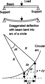
This illustrates how differential calculus may be used in the analysis of a beam which is deflected in one plane as a result of loading. Consider a beam which is bent into a circular arc and the radius R of the arc. For a segment of circular arc (Figure 4.9), the angle δθ subtended at the centre is related to the arc length δs by δs = Rδθ. Because the deflections obtained with beams are small δx is a reasonable approximation to δs and so we can write δx = Rδθ and 1/R = δθ/δx. The slope of the straight line joining the two end points of the arc is δy/δx and thus tan δθ = δy/δx. Since the angle will be small we can make the approximation that δθ = δy/δx. Hence:
In the limit we can thus write:
When a beam is bent as a result of the application of a bending moment M it curves with a radius R given by the general bending equation as:
where E is the modulus of elasticity and I the second moment of area (a property of the shape of the beam) and so we can write:
This differential equation provides the means by which the deflections of beams can be determined.
In Section 4.1.3 the determination of maximum and minimum points is discussed. We can use the criteria for a maximum in order to determine the conditions necessary for the deflection of the beam to be a maximum. In Section 4.2 we then use the above differential equation, with the condition for maximum deflection, to determine the maximum deflection of a beam.
4.1.4 Maxima and minima
There are many situations in engineering where we need to establish maximum or minimum values. For example, with a projectile we might need to determine the maximum height reached. With an electrical circuit we might need to determine the condition for maximum power to be dissipated.
Consider a graph of y against x when the values of y depend in some way on the values of x. Points on the graph at which dy/dx = 0 are called turning points and can be:
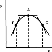
The term local is used because the value of y is only necessarily a maximum for points in the locality and there could be higher values of y elsewhere on the graph. Figure 4.10 shows such a maximum. At the maximum point A we have zero gradient for the tangent, i.e. dy/dx = 0. Consider two points P and Q close to A, with P having a value of x less than that at A and Q having a value greater than that at A. The gradient of the tangent at P is positive, the gradient of the tangent at Q is negative. Thus for a maximum we have the gradient changing from being positive prior to the turning point to negative after it.
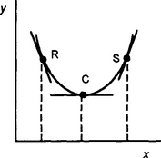
The term local is used because the value of y is only necessarily a minimum for points in the locality and there could be lower values of y elsewhere on the graph. Figure 4.11 shows such a minimum. At the minimum point C we have zero gradient for the tangent, i.e. dy/dx = 0. Consider two points R and S close to A, with R having a value of x less than that at C and S having a value greater than that at C. The gradient of the tangent at R is negative, the gradient of the tangent at S is positive. Thus for a minimum we have the gradient changing from being negative prior to the turning point to positive after it.
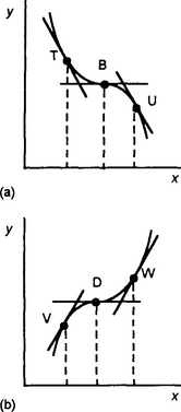
Consider points of inflexion, as illustrated in Figure 4.12. At such points dy/dx = 0. However, in neither of the graphs is there a local maximum or minimum. In Figure 4.12(a), the gradient at a point T prior to the point is negative and the gradient at a point U after the point is also negative. In Figure 4.12(b), the gradient at a point V prior to the point is positive and the gradient at a point W after the point is also positive. For a point of inflexion the sign of the gradient prior to the point is the same as that after the point.
The gradient at a point on a graph is given by dy/dx. We can thus determine whether a turning point is a maximum, a minimum or a point of inflexion by considering how the value of dy/dx changes for a value of x smaller than the turning point value compared to that for a value of x greater than the turning point value.
There is an alternative method we can use to distinguish between maximum and minimum points. We need to establish how the gradient changes in going from points before to after turning points. Consider, for a maximum, a graph of the gradients plotted against x (Figure 4.13(a)). The gradients prior to the maximum are positive and decrease in value to become zero at the maximum. They then become negative and as x increases become more and more negative. The second derivative d2y/dx2 measures the rate of change of dy/dx with x, i.e. the gradient of the dy/dx graph. The gradient of the gradient graph is negative before, at and after the maximum point. Hence at a maximum d2y/dx2 is negative.
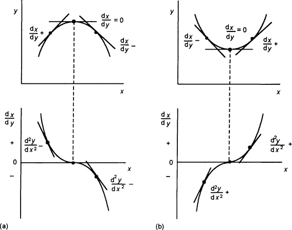
Consider a minimum (Figure 4.13(b)). The gradients prior to the minimum are negative and become less negative until they become zero at the minimum. As x increases beyond the minimum the gradients become positive, increasing in value as x increases. The second derivative d2y/dx2 measures the rate of change of dy/dx with x, i.e. the gradient of the dy/dx graph. The gradient of the gradient graph is positive before, at and after the minimum point. Hence at a minimum d2y/dx2 is positive.
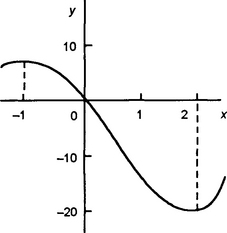
Determine, and identify the form of, the turning points on a graph of the equation y = 2x3 − 3x2 − 12x.
Differentiating the equation gives
Thus the gradient of the graph is zero when 6x2 − 6x − 12 = 0. We can rewrite this as:
The gradient is zero, and hence there are turning points, at x = −1 and x = 2.
To establish the form of these turning points consider the gradients just prior to and just after them.
Prior to the x = −1 turning point at x = −2, the gradient is 6x2 − 6x − 12 = 6 × (−2)2 − 6 × (−2) − 12 = 12. After the point at x = 0 we have a gradient of −12. Thus the gradient prior to the x = −1 point is positive and after the point it is negative. The point is thus a maximum.
Consider the x = 2 turning point. Prior to the turning point at x = 0 the gradient is −12. After the turning point at x = 3 the gradient is 6 × 32 − 6 × 3 − 12 = 24. Thus the gradient prior to the x = 2 point is negative and after the point it is positive. The point is thus a minimum.
Alternatively we could determine the form of the turning points by considering the sign of the second derivative at the points. The second derivative is obtained by differentiating the dy/dx equation. Thus
At x = −1 then the second derivative is 12 × (−1) − 6 = −18. The negative value indicates that the point is a maximum. At x = 2 the second derivative is 12 × 2 − 6 = 18. The positive value indicates that the point is a maximum.
Figure 4.14 shows a graph of the equation y = 2x3 − 3x2 − 12x, showing the maximum at x = −1 and the minimum at x = 2.
The displacement y in metres of an object is related to the time t in seconds by the equation y = 5 + 4t − t2. Determine the maximum displacement.
Differentiating the equation gives:
dy/dt is 0 when t = 2 s. There is thus a turning point at the displacement y = 5 + 4 × 2 − 22 = 9 m. We need to check that this is a maximum displacement. The gradient prior to the turning point at t = 1 has the value 4 − 2 = 2. After the turning point at t = 3 it has the value 4 − 6 = −2. The gradient changes from a positive value prior to the turning point to a negative value afterwards. It is thus a maximum.
Alternatively we could have established this by determining the second derivative. Differentiating 4 − 2t gives d2y/dx2 = −2. Thus, the turning point is a maximum.
If the sum of two numbers is 40, determine the values which will give the minimum value for the sum of their squares.
Let the two numbers be x and y. Then we must have x + y = 40. We have to find the minimum value of S when we have S = x2 + y2. We need an equation which expresses the sum in terms of just one variable. Thus substituting from the previous equation gives
Differentiating this equation, then
The value of x to give a zero value for dS/dx is when 4x − 80 = 0 and so when x = 20.
We can check that this is the value giving a minimum by considering the values of dS/dx prior to and after the point. Thus prior to the point at x = 19 we have dS/dx = 4 × 19 − 80 = −4. After the point at x = 21 we have dS/dx = 4 × 21 − 80 = 4. Thus dS/dx changes from being negative to positive. The turning point is thus a minimum. Alternatively we could check that this is a minimum by obtaining the second derivative. Differentiating 4x − 80 gives d2S/dx2 = 4. Since this is positive then we have a minimum. Thus the two numbers which will give the required minimum are 20 and 20.
Determine the maximum area of a rectangle with a perimeter of 32 cm.
If the width of the rectangle is w and its length L then the area A = wL. But the perimeter has a length of 32 cm. Thus 2w + 2L = 32. If we eliminate w from the two equations:
Hence:
dA/dL is zero when 16 − 2L = 0 and so when L = 8.
We can check that this gives a maximum area by considering values of the gradient at values of L below and above 8. At L = 7 the gradient is 2 and at L = 9 it is −2. It is thus a maximum. Alternatively we could have considered the second derivative. Since d2A/dL2 = −2 and so is negative, we have a maximum.
For a maximum area we must therefore have L = 8 cm, and, after substituting this value in 2w + 2L = 32, w = 8 cm.
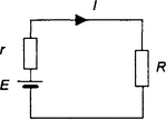
Consider the circuit shown in Figure 4.15 where a d.c. source of e.m.f. E and internal resistance r supplies a load of resistance R. The power P supplied to the load is PR with the current I being E/(R + r). Thus:
Differentiating with respect to x by using the quotient rule gives:
dP/dR = 0 when:
and so R = r. We can check that this is the condition for maximum power transfer by considering the second derivative. We have the sum of two terms and so for the E2/(R + r)2 term, let u = R + r and y = E2/u2. Then, du/dR = 1 and dy/du = −2E2/u3 and dy/dR = −2E2/(R + r)3. For y = 2E2R/(R + r)3 we can use the quotient rule to give dy/dR = [(R + r)32E2 − 2E2R3(R + r)2]/(R + r)6 which can be simplified to 2E2/(R + r)3 − 6E2R/(R + r)4. Hence:
With R = r the second derivative is negative and so we have maximum power transfer.
4.1.5 Inverse functions
If we have a function y which is a continuous function of x then the derivative, i.e. the slope of the tangent to a graph of y plotted against x, is dy/dx. However, if we have x as a continuous function of y then the derivative, i.e. the slope of the tangent to a graph of x plotted against y, is dx/dy. How are these derivatives related? We might, for example, have y = x2 and so dy/dx = 2x. For the inverse function x = √y and dx/dy = ½y−1/2.
If we have a function y = f(x) then we can write for the inverse x = g(y). Thus x = g{f(x)}. Differentiating both sides of this equation with respect to x, using the chain rule for the right-hand side, gives:
Hence, with y = f(x), the derivatives of the inverse function can be derived by using:
For example, for y = x2 we have dy/dx = 2x; the inverse function is ![]() and dx/dy = ½y−1/2. Then
and dx/dy = ½y−1/2. Then ![]()
Determine dy/dx for the function described by the equation x = y2 + 2y.
It is easier to obtain dx/dy from the equation and thus the problem is tackled by doing that operation first. Thus dx/dy = 2y + 2. Then, using equation [23]:
Problems 4.1
1. Determine the derivatives of the following functions:
2. Determine the second derivatives of the following functions:
3. Determine the velocity and acceleration after a time of 2 s for an object which has a displacement x which is a function of time t and given by x = 12 + 15t − 2t2, with t being in seconds.
4. Determine the velocity and acceleration at a time t for an object which has a displacement x in metres given by x = 3 sin 2t + 3 cos 3t, t being in seconds.
5. The voltage v, in volts, across a capacitor of capacitance 2 μF varies with time t, in seconds, according to the equation v = 3 sin 5t. Determine how the current varies with time.
6. The current i, in amps, through an inductor of inductance 0.05 H varies with time t, in seconds, according to the equation i = 10(1 − e−100t). Determine how the potential difference across the inductor varies with time.
7. The volume of a cone is one-third the product of the base area and the height. For a cone with a height equal to the base radius, determine the rate of change of cone volume with respect to the base radius.
8. The volume of a sphere of radius r is ![]() Determine the rate of change of the volume with respect to the radius.
Determine the rate of change of the volume with respect to the radius.
9. With the Doppler effect, the frequency fo heard by an observer when a sound source of frequency fs is moving away from the observer with a velocity v is given by fo = fs/(1 + v/c), where c is the velocity of sound. Determine the rate of change of the observed frequency with respect to the velocity.
10. The length L of a metal rod is a function of temperature T and is given by the equation L = Lo(1 + aT + bT2). Determine an equation for the rate of change of length with temperature.
11. Determine and identify the form of the turning points on graphs of the following functions:
12. A cylindrical container, open at one end, has a height of h m and a base radius of r m. The total surface area of the container is to be 3π m2. Determine the values of h and r which will make the volume a maximum.
13. A cylindrical metal container, open at one end, has a height of h cm and a base radius of r cm. It is to have an internal volume of 64π cm3. Determine the dimensions of the container which will require the minimum area of metal sheet in its construction.
14. The bending moment M of a uniform beam of length L at a distance x from one end is given by M = ½wLx − ½wx2, where w is the weight per unit length of beam. Determine the value of x at which the bending moment is a maximum.
15. The deflection y of a beam of length L at a distance x from one end is found to be given by y = 2x4 − 5Lx3 + 2L2x2. Determine the values of x at which the deflection is a maximum.
16. Determine the maximum value of the alternating voltage described by the equation v = 40 cos 1000t + 15 sin 1000t V.
17. The intensity of illumination from a point light source of intensity I at a distance d from it is I/d2. Determine the point along the line between two sources 10 m apart at which the intensity of illumination is a minimum if one of the sources has eight times the intensity of the other.
18. Determine the maximum rate of change with time of the alternating current i = 10 sin 1000t mA, the time t being in seconds.
19. The deflection y of a propped cantilever of length L at a distance x from the fixed end is given by:
where w is the weight per unit length and E and Is are constants. Determine the value of x at which the deflection is a maximum.
20. The e.m.f. E produced by a thermocouple depends on the temperature T and is given by E = aT + bT2. Determine the temperature at which the e.m.f. is a maximum.
21. The horizontal range R of a projectile projected with a velocity v at an angle θ to the horizontal is given by R = (v2/g) sin 2θ. Determine the angle at which the range is a maximum for a particular velocity.
22. A 100 cm length of wire is to be bent to form two squares, one with side x and the other with side y. Determine the values of x and y which give the minimum area enclosed by the squares.
23. The rate r at which a chemical reaction proceeds depends on the quantity x of a chemical and is given by r = k(a − x)(b + x). Determine the maximum rate.
24. A cylinder has a radius r and height h with the sum of the radius and height being 2 m. Determine the radius giving the maximum volume.
25. A rectangle is to have an area of 36 cm2. Determine the lengths of the sides which will give a minimum value for the perimeter.
26. An open tank is to be constructed with a square base and vertical sides and to be able to hold, when full to the brim, 32 m3 of water. Determine the dimensions of the tank if the area of sheet metal used is to be a minimum.
4.2 Integration
Integration can be considered to be the mathematical process which is the reverse of the process of differentiation. It also turns out to be a process for finding areas under graphs.
As an illustration of the application of integration in engineering as the reverse of differentiation, consider the situation where the velocity v of an object varies with time t, say v = 2t (Figure 4.14). Since velocity is the rate of change of distance x with time we can write this as:
Thus we know how the gradient of the distance–time graph varies with time. Integration is the method we can use to determine from this how the distance varies with time. We thus start out with the gradients and find the distance–time graph responsible for them, the reverse of the process used with differentiation.
4.2.1 Integration as the reverse of differentiation
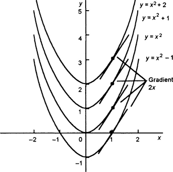
Suppose we have an equation y = x2. When this equation is differentiated we obtain the derivative of dy/dx = 2x. Thus, in this case, when given the gradient as 2x we need to find the equation which on being differentiated gave 2x. Thus, integrating 2x should give us x2. However, the derivative of x2 + 1 is also 2x, likewise the derivative of x2 + 2, the derivative of x2 + 3, and so on. Figure 4.15a shows part of the family of graphs which all have the gradients given by 2x.
Thus, for each of the graphs, at a particular value of x, such as x = 1, they all give the same gradient of 2. Thus in the integration of 2x we are not sure whether there is a constant term or not, or what value it might have. Hence a constant C has to be added to the result. Thus the outcome of the integration of 2x has to be written as being x2 + C. The integral, which has to have a constant added to it, is referred to as an indefinite integral.
To indicate the process of integration a special symbol:
is used. This sign indicates that integration is to be carried out and the dx that x is the variable we are integrating with respect to. Thus the integration referred to above can be written as
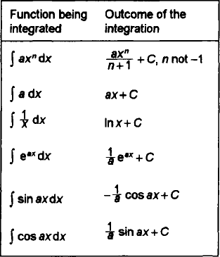
Integrals of common functions
The integrals of functions can be determined by considering what equation will give the function when differentiated. For example, consider:
Considering integration as the inverse of differentiation, the question becomes as to what function gives xn when differentiated. The derivative of xn+1 is (n + 1)xn. Thus, we have the derivative of xn+1/(n + 1) as xn. Hence:
This is true for positive, negative and fractional values of n other than n = −1, i.e. the integral of x−1. For the integral of x−1 i.e.

then since the derivative of ln x is 1/x:
This only applies if x is positive, i.e. x > 0. If x is negative, i.e. x < 0, then the integral of 1/x in such a situation is not ln x. This is because we cannot have the logarithm of a negative number as a real quantity. To show that only positive values of a quantity are to be considered, we write it as |x|.
Consider the integral of the exponential function ex, i.e.
The derivative of ex is ex. Thus:


Integral of a sum
The derivative of, for example, x2 + x is the derivative of x2 plus the derivative of x, i.e. it is 2x + 1. The integral of 2x + 1 is thus x2 + x + C. Thus, the integral of the sum of a number of functions is the sum of their separate integrals.
Finding the constant of integration
The solution given by the above integration is a general solution and includes a constant. As was indicated earlier in Figure 4.15 the integration of 2x gives y = x2 + C. This solution indicates a family of possible equations which could give dy/dx − 2x. We can, however, find a particular solution if we are supplied with information giving specific coordinate values which have to fall on the graph curve. Thus, in this case, we might be given the condition that when y = 1 we have x = 1. This must fit the equation y = x2 + C and can only be the case when C = 0. Hence the solution is y = x2.
Note that when we integrate a relationship for dy/dx with respect to x we obtain a relationship for y; when we integrate a relationship for d2y/dx2 with repect to x we obtain a relationship for dy/dx.
Determine the equation of a graph if it has to have y = 0 when x = 2 and has a gradient given by:
To obtain the general solution, i.e. the family of curves which fit the above gradient equation, we integrate. Thus:
The particular curve we require must have y = 0 when x = 2. Putting this data into the equation gives 2 = 0 + 0 + C. Hence C = 2 and so the particular solution is:
A curve is such that its gradient is described by the equation dy/dθ = cos θ and y = 1 when θ = π/2 radians. Find the equation of the curve.
Here we have the relationship dy/dθ = cos θ, and so integration gives:
This is the general solution. To find the specific equation we need to evaluate C by substituting the known conditions, namely that y = 1 when θ = π/2 radians. Thus:
Therefore C = 0 and the required equation is:
At any point on a curve we have a gradient of dy/dt = 3 sin t. Find the equation of the curve given that y = 2 when t has the value of 25°.
Given the relationship dy/dt = 3 sin t, integration gives:
The general equation is thus y = −3 cos t + C. But y = 2 when t = 25° and so:
Thus C = 4.73 and the specific equation, which is the required equation, is:
See the Maths in action in Section 4.1.3 for a preliminary discussion of the bending of beams.
The deflection y of a beam can be obtained by integrating the differential equation:
with respect to x to give:
with A being the constant of integration and then carrying out a further integration with respect to x to give:
with B being a constant of integration.
At the point where maximum deflection occurs, the slope of the deflection curve will be zero and thus the point of maximum deflection can be determined by equating dy/dx to zero.
As an illustration, consider a horizontal cantilever supporting a load at its free end (Figure 4.16). The bending moment a distance x from the fixed end is given by M = −F(L − x) and so the differential equation becomes:
Integrating with respect to x gives:
Since the slope of the beam dy/dx = 0 at the fixed end where x = 0, then we must have A = 0 and so:
Integrating again gives:
Since, at the fixed end we have zero deflection, i.e. we have y = 0 at x = 0, then we must have B = 0 and so:
When x = L:
For beams with a number of concentrated loads, there will be discontinuities in the bending moment diagram and so we cannot write a single bending moment equation to cover the entire beam but have to write separate equations for each part of the beam between adjacent loads. Integration of each expression then gives the deflections relationship for each part of the beam. There is an alternative and that involves writing a single equation using, what are termed, Macaulay’s brackets. For a discussion and examples of this method, see the companion book: Mechanical Engineering Systems by R. Gentle, P. Edwards and W. Bolton.
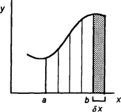
4.2.2 Integration as the area under a graph
Consider a moving object and its graph of velocity v against time t (Figure 4.17). The distance travelled between times of t1 and t2 is the area under the graph between those times. If we divide the area into a number of equal width strips then we can represent this area under the velocity–time graph as being the sum of the areas of these equal width strip areas, as illustrated in Figure 4.17. If t is the value of the time at the centre of a strip of width δt and v the velocity at this time, then a strip has an area of v δt. Thus the area under the graph between the times t1 and t2 is equal to the sum of the areas of all such strips between the times t1 and t2,
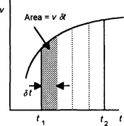

We can write this summation as:

The Σ sign is used to indicate that we are carrying out a summation of a number of terms. The limits between which this summation is to be carried out are indicated by the information given below and above the sign. If we make δt very small, i.e. let δt tend to 0, then we denote it by dt. The sum is then the sum of a series of very narrow strips and is written as:
The integral sign is an “S” for summation and the t1 and t2 are said to be the limits of the range of the variable t. Here x is the integral of the v with time t between the limits t1 and t2. The process of obtaining x in this way is termed integration. Because the integration is between specific limits it is referred to as a definite integral.
Integration as reverse of differentiation and area under a graph
The definitions of integration in terms of the reverse of differentiation and as the area under a graph describe the same concept. Suppose we increase the area A under a graph of y plotted against x by one strip (Figure 4.18). Then the increase in the area δA is the area of this strip. Thus:
with no limits specified stands for any antiderivative of f(x). When we evaluate such an integral there will be a constant in the answer.
is termed a definite integral because it takes a definite value, representing an area under a curve. When we evaluate such an integral there is no constant in the answer. The integral gives the area under the curve of the function f(x) between x = a and x = b and:
The term inside the square brackets is the result of the integration before the limits have been applied.
So we can write:
In the limit as δx tends to 0 then we can write dA/dx and so
With integration defined as the inverse of differentiation then the integration of the above equation gives the area A, i.e.
This is an indefinite integral, which is the same as that given by the definition for integration as the area under a graph when limits are imposed. An indefinite integral has no limits and the result has a constant of integration. Integration between specific limits gives a definite integral.
Areas under graphs
Consider the integration of y with respect to x when we have y = 2x. This has no specified limits and so is an indefinite integral, with the solution as the function which differentiated would give 2x:
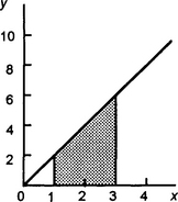
Now consider the area under the graph of y = 2x between the limits of x = 1 and x = 3 (Figure 4.19). We can write this as the definite integral:
The square brackets round the x2 + C are used to indicate that we have to impose the limits of 3 and 1 on it. Thus the integral is the value of x2 + C when x = 3 minus the value of x2 + C when x = 1.
The constant term C vanishes when we have a definite integral.: Note that an area below the x-axis is negative. If the area is required when part of it is below the x-axis then the parts below and above the x-axis must be found separately and then added, disregarding the sign of the area.
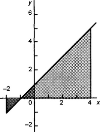
Determine the area between a graph of y = x + 1 and the x-axis between x = −2 and x = 4.
Figure 4.20 shows the graph. The area required is that between the values of x of −2 and 4. We can break this area down into a number of elements. The area under the graph between x = 0 and x = 4 is that of a rectangle 4 × 1 plus a triangle ½(4 × 4) and so is +12 square units. The area between x = −1 and 0 is that of a triangle ½(1 × 1) = 0.5 square units and the area between x = −1 and x = −2 is a triangular area below the axis and so is negative and given by ½(1 × 1) = −0.5 square units. Hence the total area under the graph is + 12 + 0.5 − 0.5 = 12 square units.
Alternatively we can consider this area as the integral:
and so:
Find the areas under the curve y = x3 between (a) x = 0 and x = 1, (b) x = −1 and x = 1.
(a) Figure 4.21 shows the graph. The area is:
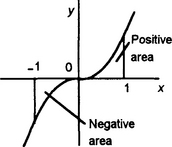
The area is zero because the area between x = −1 and x = 0 is negative. What we have is the sum of two areas:
The sum of the two areas is thus zero. If we want the total area, regardless of sign, between the axis and the curve for any function then we have to determine the positive and negative elements separately and then, ignoring the sign, add them. For this curve this gives ½.
With a constant force F acting on a body and a displacement x in the direction of the force, then the work done W on a body, i.e. the energy transferred to it, is given by W = Fx.
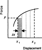
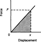
Consider a variable force described by the graph shown in Figure 4.22 for the force applied to an object and how it varies with the displacement of that object. For a small displacement δx we can consider the force to be effectively constant at F. Thus the work done for that displacement is F δx. This is the area of the strip under the force–distance graph. If we want the work done in changing the displacement from x1 to x2 then we need to determine the sum of all such strips between these displacements, i.e. the total area under the graph between the ordinates for x1 and x2. Thus:
If we make the strips tend towards zero thickness then the above summation becomes the integral, i.e.
Consider the work done in stretching a spring when a force F is applied and causes a displacement change in its point of application, i.e. an extension, from 0 to x if F = kx, where k is a constant. Figure 4.23 shows the force–distance graph.
The work done is the area under the graph between 0 and x. This is the area of a triangle and so the work done is ½Fx. Since F = kx we can write this as ½kx2.
We could have solved this problem by integration. Thus:
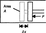
As a further illustration, consider the work done as a result of a piston in Figure 4.24 being moved to reduce the volume of a gas. The work done in moving the piston through a small distance δx when the force is F is F δx. Since pressure is force per unit area, then if the force acts over an area A the pressure p = F/A. Thus:
But A δx is the change in volume δV of the gas. Hence, the work done = p δV. The total work done in changing the volume of a gas from V1 to V2 is thus:
If we consider δV tending to zero then we can write
For a gas that obeys Boyle’s law, i.e. pV = a constant k, the work done in compressing a gas from a volume V1 to V2 is thus:
Hence the work done is ln V2 − ln V1.
Centre of gravity and centroid
The weight of a body is made up of the weights of each constituent particle, each such particle having its weight acting at a different point. However, it is possible to replace all the weight forces of an object by a single weight force acting at a particular point, this point being termed the centre of gravity.
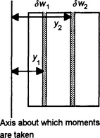
If we consider a sheet to be made of a large number of small strip elements of mass at different distances from an axis (Figure 4.25) then the weight of each element will give rise to a moment about that axis. Thus the total moment due to all the weight elements is δw1x1 + δw2x2 + δw3x3 + …. If a single weight W at a distance ![]() is to give the same moment, then:
is to give the same moment, then:
Thus the distance of the centre of gravity from the chosen axis is:

For a thin flat plate of uniform density, the weight of an element is proportional to its area. We then refer to the centroid since it is purely geometric. The distance of the centroid from the chosen axis is thus:

where δa represents the area of an elemental strip. The product of an area and its distance from an axis is known as the first moment of area of that area about the axis. Thus the centroid distance from an axis is the sum of the first moments of all the area elements divided by the sum of all the areas of the elements.
If we consider infinitesimally small elements, i.e. δa → 0, then we can write:
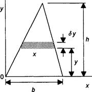
Consider the determination of the centroid of a triangular area (Figure 4.26). Consider a small strip of area δA = x δy. By similar triangles x/(h − y) = b/h and so x δy = [b(h − y)/h] δy. The total area A = ½bh. Hence, the y coordinate of the centroid is:
The centroid is located at one-third the altitude of the triangle. The same result is obtained if we consider the location with respect to the other sides. The centroid is at one-third the altitude along of the lines drawn from each apex to the opposite side.
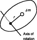
Consider a rigid body rotating with a constant angular acceleration a about some axis (Figure 4.27). We can consider the body to be made up of small elements of mass δm. For such an element a distance r from the axis of rotation we have a linear acceleration of a = rα. Thus the force acting on the element is δm × rα. The moment of this force is thus Fr = r2α δm. The total moment, i.e. torque T, due to all the elements of mass in the body is thus:
Thus if we have elements of mass at radial distance from 0 to R, in the limit as δm → 0:
Since a is a constant we can write the above equation as:
where I is the moment of inertia
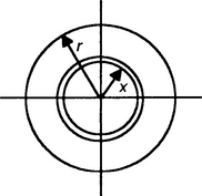
As an illustration consider the determination of the moment of inertia of a uniform disc about an axis through its centre and at right angles to its plane. Figure 4.28 shows the disc with an element of mass being chosen as a disc with a radius x and width δx. The element is a strip of length 2πx and so an area of 2πx δx. If the mass of the disc is m per unit area, then the mass of the element is δm = 2πmx δx. The moment of inertia of the element is x2 δm = 2πmx3 δx. Thus the moment of inertia of the disc is:
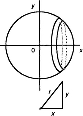
As another illustration, consider a sphere of radius r and mass per unit volume m. If we take a thin slice of thickness δx of the sphere perpendicular to the diameter about which the moment of inertia is to be determined and a distance x from the sphere centre (Figure 4.29), then with the slice radius y we have an element of volume πy2 δx and hence mass πmy2 δx. The moment of inertia of a disc is ½ mass × radius2 (see the previous example) and thus the moment of inertia of the slice is ½(πmy2 δx)y2 and the moment of inertia of the sphere as the sum of all the slices as δx → 0 is:
The total mass M of the sphere is ![]() so
so ![]()
Consider a beam that has been bent into the arc of a circle so that the uppermost surface is in tension and the lower surface in compression (Figure 4.30). The upper surface has increased in length and the lower surface decreased in length; between the two there is a plane which is unchanged in length; this is called the neutral plane and the line where the plane cuts the cross-section of the beam is the neutral axis.
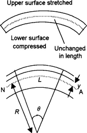
Figure 4.30 Bending stretches the upper surface and contracts the lower surface, in-between there is an unchanged in length surface
An initially horizontal plane through the beam which is a distance y from the neutral axis changes in length as a consequence of the beam being bent and the strain it experiences is the change in length ΔL divided by its initial unstrained length L. For circular arcs, the arc length is the radius of the arc multiplied by the angle it subtends, and thus, L + ΔL = (R + y)θ. The neutral axis NA will, by definition, be unstrained and so for it we have L = Rθ. Hence, the strain on aa is:
Provided we can use Hooke’s law, the stress due to bending which is acting this plane is:
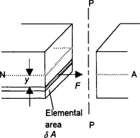
Looking at a cross-sectional slice of the beam cut by PP we have Figure 4.31. The moment M of the elemental force F about the neutral axis is Fy and the stress σ acting on the elemental area is F/δA. Therefore the moment is (σ δA)y. Hence, using the equation we derived above for the stress, the moment of this element about the neutral axis is:
The total moment M produced over the entire cross-section is the sum of all the moments produced by all the elements of area in the cross-section. Thus, if we consider each such element of area to be infinitesimally small, we can write:
The integral is termed the second moment of area I of the section:
Thus we can write:
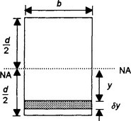
For a rectangular cross-section of breadth b and depth d (Figure 4.32) with a segment of thickness δy a distance y from the neutral axis, the second moment of area for the segment is:
The total second moment of area for the section about the neutral axis is thus:
4.2.3 Techniques for integration
There are a number of techniques which can aid in the integration of functions. In this section we look at integration by substitution, integration by parts and partial fractions.
Integration by substitution
This involves simplifying integrals by making a substitution. The term integration by change of variable is often used since the variable has to be changed as a result of the substitution. The aim of making a substitution is to put the integral into a simpler form for integration. As an illustration, consider the integral:
The substitution u = 5x reduces e5x to eu. However, we also need to change dx in the variable to du for the integration. Since du/dx = 5, we can write the integral as:
∫ cosm ax sinn ax dx, when n is od
Let u = cos ax. Use sin2 ax + cos2 ax = 1 in the simplification.
∫ cosm ax sinn ax dx, when m is od
Let u = cos ax. Use sin2 ax + cos2 ax = 1 in the simplification.
∫ cosm ax sinn ax dx, when m and are both even or both odd Rewrite the integral using:
In the above case the substitution of u for 5x seemed a sensible way to simplify the integral. However, there are no general rules for finding suitable substitutions and the key points show some of the more commonly used substitutions.
Determine the indefinite integral ![]()
If we let u = 3x2 + 4, then du/dx = 6x and so x dx = (1/6) du. Hence:
The modulus sign is used with the integration of 1/u because no assumption is made at that stage as to whether u is positive or negative. The sign is dropped when the substitution is made because 3x2 + 4 is always positive.
Trigonometric substitutions
A useful group of substitutions is to use trigonometric functions. For example, for integrals involving √(a2 − x2) terms, we can use the substitution x = a sin θ. Then √(a2 − x2) = √(a2 − a2 sin2 θ) = a cos θ, since we have 1 − sin2 θ = cos2 θ. Since dx/dθ = a cos θ then a cos θ dθ. The key points give other such substitutions.
Determine the indefinite integral ![]()
Let x = sin θ. Then √(1 − x2) = √(1 − sin2 θ) = cos θ. Since dx/dθ = cos θ then dx = cos θ dθ. Thus the integral becomes:
Since cos 2θ = 2 cos2 θ − 1, we have:
Back substitution using θ = sin−1 x gives:
However, a simpler expression is obtained if we first replace the sin 2θ using sin 2θ = 2 sin θ cos θ = 2sinθ √(1 − sin2 θ).
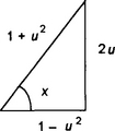
Another form of useful substitution, when we have integrals involving sin x, cos x, tan x terms, is to let u = tan ½x. Then du/dx = ½ sec2 ½x. But sec2 x = 1 + tan2 x, thus du/dx = ½(1 + tan2 x) = ½(1 + u2). Thus dx = 2 du/(1 + u2). The trigonometric functions can all be expressed in terms of u. Thus:
Figure 4.33 shows the right-angled triangle with such an angle. Hence:
Note that integration of the squares of trigonometric functions can be obtained by using trigonometric identities to put the functions in non-squared form. Thus:

Substitution with definite integrals
The above has discussed the substitution procedure with indefinite integrals where the variable was changed from x to u. When we have definite integrals we can do the same procedure and take account of the limits of integration at the end after reversing the substitution. The limits are in terms of values of x. However, it is often simpler to express the limits in terms of u and take account of the limits before reversing the substitution. To illustrate this, consider the integration of cos3 x between the limits 0 and ½π. If we let u = sin x then du/dx = cos x and so cos x dx = du. When x = 0 then u = 0 and when x = ½π then u = 1. Thus the integral can be written as:
Integration by parts
The product rule for differentiation gives:
Integrating both sides of this equation with respect to x gives:
Hence:
This is the formula for integration by parts. This is often written in terms of u = f(x) and v = g(x) as:
With a definite integral the equation becomes:
Determine the indefinite integral ∫ x ex dx.
The integral consists of the product of two factors. If we let u = x and dv/dx = ex, then v = ∫ex dx and equation [32] gives:
Integration by partial fractions
Integrals involving fractions can often by simplified by expressing the integral as the sum or difference of two or more partial fractions which then lend themselves to easier integration. For example:
can be expressed as the partial fractions:
When the degree of the denominator is greater than that of the numerator then an expression can be directly resolved into partial fractions. The form taken by the partial fractions depends on the type of denominator concerned.
• If the denominator contains a linear factor, i.e. a factor of the form (x + a), then for each such factor there will be a partial fraction of the form:
where A is some constant.
• If the denominator contains repeated linear factors, i.e. a factor of the form (x + a)n, then there will be partial fractions:
with one partial fraction for each power of (x + a).
• If the denominator contains an irreducible quadratic factor, i.e. a factor of the form ax2 + bx + c, then there will be a partial fraction of the form:
for each such factor.
• If the denominator contains repeated quadratic factors, i.e. a factor of the form (ax2 + bx + c)n, there will be partial fractions of the form:
with one for each power of the quadratic.
The values of the constants A, B, C, etc. can be found by either making use of the fact that the equality between the fraction and its partial fractions must be true for all values of the variable x or that the coefficients of xn in the fraction must equal those of xn when the partial fractions are multiplied out.
When the degree of the denominator, i.e. the power of its highest term, is equal to or less than that of the numerator, the denominator must be divided into the numerator until the result is the sum of terms with the remainder fraction term having a denominator which is of higher degree than its numerator. Consider, for example, the fraction:
The numerator has a degree of 3 and the denominator a degree of 2. Thus, dividing has to be used. Thus
The fractional term can then be simplified using partial fractions.
to give:
Simplify into its partial fraction form: ![]()
This has two linear factors in the denominator and so the partial fractions are of the form:
with one partial fraction for each linear term. Thus for the expressions to be equal we must have:
Thus
Consider the requirement that this relationship is true for all values of x. Then, when x = −1 we must have:
Hence A = 1. When x = −2 we must have:
Hence B = 2.
Alternatively, we could have determined these constants by multiplying out the expression and considering the coefficients, i.e.
Thus, for the coefficients of x to be equal we must have 3 = A + B and for the constants to be equal 4 = 2A + B. These two simultaneous equations can be solved to give A and B. The partial fractions are thus:
Determine the indefinite integral ![]()
The fraction 1/(x2 − 1) can be written as:
Hence, equating coefficients of x gives A + B = 0 and equating integers gives A − B = 1. Thus A = ½ and B = −½. Hence the integral can be expressed as:
We can determine these integrals by substitution. Thus if we let u = x − 1 then du/dx = 1 and so:
Likewise the integral of 1/(x + 1) is ln |x + 1| + B. Hence:

Determine the indefinite integral 
Expressed as partial fractions:
Equating the constant terms gives A = 1. Equating the coefficients of x gives C = 0. Equating the coefficients of x2 gives A + B = 0, and so B = −1. Thus the integral becomes:
The integration of 1/(x2 + 1) can be carried out by using a substitution. Let u = x2 + 1 and so du/dx = 2x. Thus:
and so:
The technique of using partial fractions to simplify expressions has many uses. In chapter 6, we shall see how partial fractions can help in the solution of differential equations using the Laplace transform. As an illustration, consider a differential equation relating rotational displacement θ to time t for a rotating power transmission shaft:
Given that when t = 0 we have θ = 4 and dθ/dt = 25/2, the Laplace transform enables the differential equation to be written in the form:
We can use the method of partial fractions to simplify the expression. Let the fraction be replaced by:
If we let s = 2, then 32 − 78 + 84 − 40 = B(2)(4 − 12 + 10) and so B = −1/2. If we let s = 0, then −40 = A(−2)(10) and so A = 2. Comparing coefficients of s gives 42 = 22A + 10B − 2D and so D = −3/2. Comparing coefficients of s3 gives 4 = A + B + C and so C = 5/2. Putting these values into the partial fraction equation gives:
This is a lot easier to handle than the original equation.
4.2.4 Means
The mean of a set of numbers is their sum divided by the number of numbers summed. The mean value of a function between x = a and x = b is the mean value of all the ordinates between these limits. Suppose we divide the area into n equal width strips (Figure 4.34), then if the values of the mid-ordinates of the strips are y1, y2, … yn the mean value is:
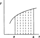
If δx is the width of the strips, then n δx = b − a. Thus:
Hence, as δx → 0:
Since the sum of all the y δx terms is the area under the graph between x = a and x = b:
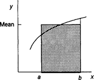
But the product of the mean value and (b − a) is the area of a rectangle of height equal to the mean value and width (b − a). Figure 4.35 shows this mean value rectangle.
Root-mean-square values
The power dissipated by an alternating current i when passing through a resistance R is i2R. The mean power dissipated over a time interval from t = 0 to t = T will thus be:
If we had a direct current I generating the same power then we would have:
and:
This current I is known as the root-mean-square current. There are other situations in engineering and science where we are concerned with determining root-mean-square quantities. The procedure is thus to determine the mean value of the squared function over the required interval and then take the square root.
Determine the root-mean-square value of the waveform shown in Figure 4.36 over a period of 0 to 2 s.
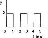
From t = 0 to t = 1 s the waveform is described by y = 2. From t = 1 s to t = 2 s the waveform is described by y = 0. Thus the root-mean-square value is given by:
An alternating current is defined by the equation:
Determine its mean value over half-a-cycle and the root-mean-square value over a cycle.
We have 100π = 2πf = 2π/T, where f is the frequency and T the periodic time. Hence the periodic time is 0.02 s and the time for half-a-cycle is 0.01 s.
Using equation [34], the mean value over half-a-cycle is:
We can use the standard form for the integral of sin ax to give the mean value as:
Thus the mean value over half-a-cycle is 15.92 mA. Note that for a sinusoidal signal the mean value over a full cycle is zero.
The root-mean-square value over a cycle is given by equation [35] as:
Since sin2θ = ½(1 − cos 2θ), we can write:
and so the r.m.s. current 25/√2 = 17.68 mA. Note, that in general, the root-mean-square value of a sinusoidal signal is always the maximum value divided by √2.
Problems 4.2
1. Determine the integrals of the following:
2. Determine the areas under the following curves between the specified limits and the x-axis:
(a) y = 4x3 between x = 1 and x = 2,
(b) y = x between x = 0 and x = 4,
(c) y = 1/x between x = 1 and x = 3,
(d) y = x3 − 3x2 − 2x + 2 between x = −1 and x = 2,
(e) y = x2 − x − 2 between x = −1 and x = 2,
(f) y = x2 − 1 between x = −1 and x = 2,
(g) the area between x = 0 and x = 2 for the curve defined by y = x2 between x = 0 and x = 1 and by y = 2 − x between x = 1 and x = 2.
3. Determine the areas bounded by graphs of the following functions and between the specified ordinates:
4. Determine the geometrical area enclosed between the graph of the function y = x(x − 1)(x − 2) and the x-axis.
5. Determine the area bounded by graphs of y = x3 and y = x2.
6. Determine the area bounded by the graph of y = sin x, the x-axis and the line x = π/2.
7. Determine the area bounded by graphs of y = x2 − 2x + 2 and y = 4 − x.
8. Determine the values, if they exist, of the following definite integrals:

9. Determine the following indefinite integral by using the given substitutions:
10. Determine the following indefinite integrals by making appropriate substitutions:
11. By making appropriate substitutions, evaluate the following definite integrals:
12. Using the method of integration by parts, determine the following indefinite integrals:
13. Using the method of integration by parts, evaluate the following definite integrals:
14. Determine the following indefinite integrals:
15. Determine the moment of inertia for a uniform triangular sheet of mass M, base b and height h about (a) an axis through the centroid and parallel to the base and (b) about the base. The centroid is at one-third the height.
16. Determine the moment of inertia of a flat circular ring with an inner radius r, outer radius 2r and mass M about an axis through its centre and at right angles to its plane.
17. Determine the moment of inertia of a uniform square sheet of mass M and side L about (a) an axis through its centre and in its plane, (b) an axis in its plane a distance d from its centre.
18. Determine the mean values of the following functions between the specified limits:
(a) y = 2x between x = 0 and x = 1,
(b) y = x2 between x = 1 and x = 4,
19. With simple harmonic motion, the displacement x of an object is related to the time t by x = A cos ωt. Determine the mean value of the displacement during one-quarter of an oscillation, i.e. between when ωt = 0 and ωt = o.
20. The number N of radioactive atoms in a sample is a function of time t, being given by N = N0 e−λt. Determine the mean number of radioactive atoms in the sample between t = 0 and t = 1/λ.
21. Determine the root-mean-square values of the following functions between the specified limits:
(a) y = x2 from x = 1 to x = 3,
(b) y = x from x = 0 to x = 2,
(c) y = sin x + 1 from x = 0 to x = 2π,
22. Determine the root-mean-square value of a half-wave rectified sinusoidal voltage. Between the times t = 0 and t = π/ω the equation is v = V sin ωt and between t = π/ω and t = 2π/ω we have v = 0.