
Probability and statistics
9.1 Probability
What is the chance an engineering system will fail? What is the chance that a product emerging from a production line is manufactured to the required engineering tolerances, thus avoiding reworking or scrap? What is the chance that if you make a measurement in some experiment that it will be the true value of that quantity? Within what range of experimental error might you expect a measurement to be the true value? These, and many other questions in engineering and science, involve a consideration of chances of events occurring. The term probability is more often used in mathematics than chance and has the same meaning in the above questions. This section is about probability, its definition and determination in a number of situations.
9.1.1 Basic definitions
If you flip a coin into the air, what is the chance that it will land heads uppermost? We can try such an experiment and determine the outcomes. The result of a large number of trials leads to the result that about half the time it lands heads uppermost and half the time tails uppermost. If n is the number of trials then we can define probability P as:
This view of probability is the relative frequency in the long run with which an event occurs. In the case of the coin this leads to a probability of ½ = 0.5. If an event occurs all the time then the probability is 1. If it never occurs the probability is 0.
The result of flipping the coin might seem obvious since there are just two ways a coin can land and just one of the ways leads to heads uppermost. If there is no reason to expect one way is more likely than the other then we can define probability P as the degree of uncertainty about the way an event can occur and as:
In the case of the coin, this also gives a probability of 0.5. If every possible way events can occur is the required way, then the probability is 1. If none of the possible ways are the event required, then the probability is 0.
Consider a die-tossing experiment. A die can land in six equally likely ways, with uppermost 1, 2, 3, 4, 5, or 6. Of the six possible ways the die could land, only one way is with 6 uppermost. Thus using definition [2], the probability of obtaining a 6 is 1/6. The probability of not obtaining a 6 is 5/6 since there are 5 ways out of the 6 possible ways we can obtain an outcome which is not a 6.
Another way the term probability is used is as degree of belief. Thus we might consider the probability of a particular horse winning a race as being 1 in 5 or 0.2. The probability in this case is highly subjective.
Probability of events
If an event can occur in two possible ways, e.g. a piece of equipment can be either operating satisfactorily or have failed, then if the probability of one way is P1 and the probability of the other way is P2, we must have:
The probability of either event 1 or event 2 occurring equals 1, i.e. a certainty, and is the sum of the probability of event 1 occurring, i.e. P1, added to the probability of event 2, i.e. P2, occurring.
Suppose with the die-tossing experiment we were looking for the probability that the outcome would be an even number. Of the six possible outcomes of the experiment, three ways give the required outcome. Thus, using definition [2], the probability of obtaining an even number is 3/6 = 0.5. This is the sum of the probabilities of 2 occurring, 4 occurring and 6 occurring, i.e. 1/6 + 1/6 + 1/6. The 2, the 4 and the 6 are mutually exclusive events in that if the 2 occurs then 4 or 6 cannot also be occurring. Thus:
If A and B are mutually exclusive, the probability of A or B occurring is the sum of the probabilities of A occurring and of B occurring.
9.1.2 Ways events can occur
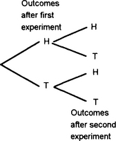
Suppose we flip two coins. What is the probability that we will end up with both showing heads uppermost? The ways in which the coins can land are:
There are four possible results with just one of the ways giving HH. Thus the probability of obtaining HH is ¼ = 0.25.
There were two possible outcomes from the experiment of tossing the first coin and two possible outcomes from the experiment of tossing the second coin. For each of the outcomes from the first experiment there were two outcomes from the second experiment. Thus for the two experiments the number of possible outcomes is 2 × 2 = 4. This is an example of, what is termed, the multiplication rule.
Tree diagrams can be used to visualise the outcomes in such situations, Figure 9.1 showing this for the two experiments of tossing coins.
A company is deciding to build two new factories, one of them to be in the north and one in the south. There are four potential sites in the north and two potential sites in the south. Determine the number of possible outcomes.
For the first experiment there are 4 possible outcomes A, B, C and D and for the second 2 possible outcomes E and F. Thus the total number of possible outcomes is given by the multiplication rule as 8. Figure 9.2 shows the tree diagram.

Permutations
Suppose we had to select two items from a possible three different items A, B, C. The first item can be selected in three ways. Then, since the removal of the first item leaves just two remaining, the second item can be selected in two ways. Thus the selections we can have are:
Each of the ordered arrangements is known as a permutation, each representing the way distinct objects can be arranged.
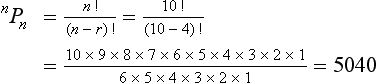
If there are n ways of selecting the first object, there will be (n − 1) ways of selecting the second object, (n − 2) ways of selecting the third object and (n − r + 1) ways of selecting the rth object. Thus, by the multiplication rule, the total number of different permutations of selecting r objects from n distinct objects is thus:
The number n(n − 1)(n − 2) … (3)(2)(1) is represented by n!. The number of permutations of k objects chosen from n distinct objects is represented by nPr or nPr or ![]() and is thus:
and is thus:
r taking values from 0 to n. Note that 0! is taken as having the value 1. The number of permutations of n objects chosen from n distinct objects is represented by nPn or ![]() and is thus:
and is thus:
In the wiring up of an electronic component there are four assemblies that can be wired up in any order. In how many different ways can the component be wired?
This involves determining the number of permutations of four objects from four. Thus, using equation [5]:
How many four-digit numbers can be formed from the digits 0 to 9 if no digit is to be repeated within any one number?
This involves determining the number of permutations of 4 objects from 10. Thus, using equation [4]:
Combinations
There are often situations where we want to know the number of ways r items can be selected from n objects without being concerned with the order in which the objects are selected. Suppose we had to select two items from a possible three different items A, B, C. The selections, i.e. permutations, we can have are:
But if we are not concerned with the sequence of the letters then we only have the three ways AB, AC and BC. Such an unordered set is termed a combination.
Consider the selection of a combination of r items from n distinct objects. In the selected r items there will be r! permutations (equation [5]) of distinct objects so that the permutation of r items from n contains each group of r items r! times. Since there are n!/(n − r)! different permutations of r items from n we must have:
where nCr, nCr or ![]() is used to represent the combination of r items from n. Thus:
is used to represent the combination of r items from n. Thus:
nCr is often termed a binomial coefficient. This is because numbers of this form appear in the expansion of (x + y)n by the binomial theorem (see Section 7.1.2).
When r items are selected from n distinct objects, n − r items are left. The number of ways of selecting r items from n is given by equation [6] as n!/r!(n − r)!. The number of ways of selecting n − r items from n is given by equation [6] as:
Thus we can say that there are as many ways of selecting r items from n as selecting n − r objects from n:
There is just one combination of n items from n objects. Thus nCn = 1. If we select 0 items from n, then because equation [6] gives nC0 = n!/0! and we take 1/0! = 1, we have nC0 = 1. Evidently there are as many ways of selecting none of the items in a set of n as there are of choosing the n objects that are left.
If a batch of 20 objects contains 3 with faults and a sample of 5 is chosen, what is the probability of obtaining a sample with (a) 0, (b) 1, (c) 2 faulty items?
The number of ways we choose the sample of 5 items out of 20 is, using equation [6]:
(a) The number of ways we can choose a sample with 0 defective items is the number of ways we choose 5 items from 17 good items and is thus:
Thus the probability of choosing a sample with 0 faulty items is:
(b) The number of ways we can choose a sample with 1 faulty item and 4 good items, i.e. selecting 1 faulty item from 3 faulty items and 4 good items from 17 good items, is given by the multiplication rule as 3C1 × 17C4. Thus the probability of choosing a sample with 1 faulty item is:

(c) The number of ways we can choose a sample with 2 faulty items and 3 good items, i.e. selecting 2 faulty items from 3 faulty items and 3 good items from 17 good items, is given by the multiplication rule as 3C2 × 17C3. Thus the probability of choosing a sample with 2 faulty items is:

Conditional probability
The multiplication rule is only valid when the occurrence of one event has no effect upon the probability of the second event occurring. While this can be used in many situations, there are situations where a successful occurrence of the first event affects the probability of occurrence of the second event. Suppose we have 50 objects of which 15 are faulty. What is the probability that the second object selected is faulty given that the first object selected was fault-free? This is a probability problem where the answer depends on the additional knowledge given that the first selection was fault-free. This means that there are less fault-free objects among those remaining for the second selection. Such a problem is said to involve conditional probability.
Problems 9.1
1. In a testing period of 1 year, 4 out of 50 of the items tested failed. What is the probability of finding one of the items failing?
2. In a pack of 52 cards there are 4 aces. What is the probability of selecting, at random, an ace from a pack?
3. Testing of a particular item bought for incorporation in a product shows that of 100 items tested, 4 were found to be faulty. What is the probability that one item taken at random will be (a) faulty, (b) free from faults?
4. Resistors manufactured as 10 Ω by a company are tested and 5% are found to have values below 9.5 Ω and 10% above 10.5 Ω. What is the probability that one resistor selected at random will have a resistance between 9.5 Ω and 10.5 Ω?
5. 100 integrated circuits are tested and 3 are found to be faulty. What is the probability that one, taken at random, will result in a working circuit?
6. Tests of an electronic product show that 1% have defective integrated circuits alone, 2% have defective connectors alone and 1% have both defective integrated circuits and connectors. What is the probability of one of the products being found to have a (a) defective integrated circuit alone, (b) defective integrated circuit, (c) defective connector, (d) no defects?
7. Cars coming to a junction can turn to the left, to the right or go straight on. If observations indicate that all the possible outcomes are equally likely, determine the probability that a car will (a) go straight on, (b) turn from the straight-on direction.
8. In how many ways can (a) 8 items be selected from 8 distinct objects, (b) 4 items be selected from 7 distinct items, (c) 2 items be selected from 6 distinct items?
9. In how many ways can (a) 2 items be selected from 7 objects, (b) 5 items be selected from 7 objects, (c) 7 items be selected from 7 objects?
10. How many samples of 4 can be taken from 25 items?
11. A batch of 24 components includes 2 that are faulty. If a sample of 2 is taken, what is the probability that it will contain (a) no faulty components, (b) 1 faulty component, (c) 2 faulty components?
12. A batch of 10 components includes 3 that are faulty. If a sample of 2 is taken from the batch, what is the probability that it will contain (a) no faulty components, (b) 2 faulty components?
13. Of 10 items manufactured, 2 are faulty. If a sample of 3 is taken at random, what is the probability it will contain (a) both the faulty items, (b) at least 1 faulty item?
14. A security alarm system is activated and deactivated by keying-in a three-digit number in the proper sequence. What is the total number of possible code combinations if digits may be used more than once?
15. When checking on the computers used in a company it was found that the probability of one having the latest microprocessor was 0.8, the probability of having the latest software 0.6 and the probability of having the latest processor and latest software 0.3. Determine the probability that a computer selected as having the latest software will also have the latest microprocessor.
9.2 Distributions
All measurements are affected by random uncertainties and thus repeated measurements will give readings which fluctuate in a random manner from each other. This section considers the statistical approach to such variability of data, dealing with the measures of location and dispersion, i.e. mean, standard deviation and standard error, and the binomial, Poisson and Normal distributions. This statistical approach to variability is especially important in the production environment and the consideration of the variability of measurements made on products.
9.2.1 Probability distributions
Consider the collection of data on the number of cars per hour passing some point and suppose we have the following results:
When the discrete variable is sampled 10 times the value 10 appears once. Thus the probability of 10 appearing is 1/10. The value 11 appears three times and so its probability is 3/10, 12 has a probability of 4/10, 13 has the probability 1/10, 14 has the probability 1/10. Figure 9.3 shows how we can represent these probability values as a probability distribution.

Consider some experiment in which repeated measurements are made of the time taken for 100 oscillations of a simple pendulum and suppose we have the following results:
With a continuous variable there are an infinite number of values that can occur within a particular range so the probability of one particular value occurring is effectively zero. However, it is meaningful to consider the probability of the variable falling within a particular subinterval. The term frequency is used for the number of times a measurement occurs within an interval and the term relative frequency or probability P(x) for the fraction of the total number of readings in a segment. Thus if we divide the range of the above results into 0.2 intervals, we have:
values >20.0 and ≤20.2 come up twice, thus P(x) = 2/20
values >20.2 and ≤20.4 come up five times, thus P(x) = 5/20
values >20.4 and ≤20.6 come up seven times, thus P(x) = 7/20
The probability always has a value less than 1 and the sum of all the probabilities is 1. Figure 9.4 shows how we can represent this graphically. The probability that x lies within a particular interval is thus the height of the rectangle for that strip divided by the sum of the heights of all the rectangles. Since each strip has the same width w:
The histogram shown in Figure 9.4 has a jagged appearance. This is because it represents only a few values. If we had taken a very large number of readings then we could have divided the range into smaller segments and still had an appreciable number of values in each segment. The result of plotting the histogram would now be to give one with a much smoother appearance. When the probability distribution graph is a smooth curve, with the area under the curve scaled to have the value 1, then it is referred to as the probability density function f(x) (Figure 9.5). Then equation [8] gives:


Consider the probability, with a very large number of readings, of obtaining a value between 20.8 and 21.0 with the probability distribution function shown in Figure 9.6. If we take a segment 20.8 to 21.0 then the area of that segment is the probability. If, say, the area is 0.30, the probability of taking a single measurement and finding it in that interval is 0.30, i.e. the measurement occurs on average 30 times in every 100 values taken.

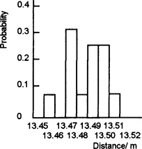
The following readings, in metres, were made for a measurement of the distance travelled by an object in 10 s. Plot the results as a distribution with segments of width 0.01 m.

With segments of width 0.01 m we have:
Segment 13.45 to 13.46, frequency 1, so probability 1/16
Segment 13.46 to 13.47, frequency 0, so probability 0
Segment 13.47 to 13.48, frequency 5, so probability 5/16
Segment 13.48 to 13.49, frequency 1, so probability 1/16
Segment 13.49 to 13.50, frequency 4, so probability 4/16
Figure 9.7 shows the resulting distribution.
9.2.2 Measures of location and spread of a distribution
Parameters which can be specified for distributions to give an indication of location and a measure of the dispersion or spread of the distribution about that value are the mean for the location and the standard deviation for the measure of dispersion.
Mean
The mean value of a set of readings can be obtained in a number of ways, depending on the form with which the data is presented:
• For a list of discrete readings, sum all the readings and divide by the number N of readings, i.e.:
• For a distribution of discrete readings, if we have n1 readings with value x1, n2 readings with value x2, n3 readings with value x3, etc., then the above equation for the mean becomes:
But n1/N is the relative frequency or probability of value x1, n2/N is the relative frequency or probability of value x2, etc. Thus, to obtain the mean, multiply each reading by its relative frequency or probability P and sum over all the values:
• For readings presented as a continuous distribution curve, we can consider that we have a discrete-value distribution with very large numbers of very thin segments. Thus if f(x) represents the probability distribution and x the measurement values, the probability that x will lie in a small segment of width δx is f(x)δx. Thus the rule given above for discrete-value distributions translates into:
With a very large number of readings, the mean value is taken as being the true value about which the random fluctuations occur. The mean value of a probability distribution function is often termed the expected value.
Standard deviation
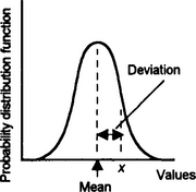
Any single reading x in a distribution (Figure 9.8) will deviate from the mean of that distribution by:
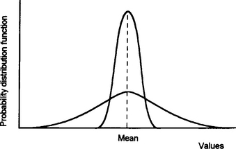
With one distribution we might have a series of values which is widely scattered around the mean while another has readings closely grouped round the mean. Figure 9.9 shows the type of curves that might occur.
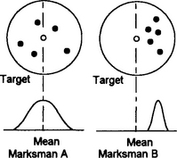
Consider two marksmen firing 5 shots, from the same gun under the same conditions, at a target with the aim of hitting the central bulls-eye. If the results obtained are as shown in Figure 9.10, then marksman A is accurate in that his shots have a mean which coincides with the bulls-eye. Marksman B has a smaller scatter of results but his mean is not centres on the bulls-eye. His shots have greater precision but are less accurate. Dispersion measurement is thus extremely important when designing manufacturing processes and machining to a set target mean value, i.e. the bulls-eye, with attainable tolerances.
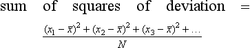
A measure of the spread of a distribution cannot be obtained by taking the mean deviation from the mean, since for every positive value of a deviation there will be a corresponding negative deviation and so the sum will be zero. The measure used is the standard deviation.
The standard deviation σ is the root-mean-square value of the deviations for all the measurements in the distribution. The quantity σ 2 is known as the variance of the distribution.
Thus, for a number of discrete values, x1, x2, x3, …, etc., we can write for the mean value of the sum of the squares of their deviations from the mean of the set of results:
Hence the mean of the square root of this sum of the squares of the deviations, i.e. the standard deviation, is:
However, we need to distinguish between the standard deviation s of a sample and the standard deviation σ of the entire population of readings that are possible and from which we have only considered a sample (many statistics textbooks adopt the convention of using Greek letters when referring to the entire population and Roman for samples). When we are dealing with a sample we need to write:
with ![]() being the mean of the sample. The reason for using N − 1 rather than N is that the root-mean-square of the deviations of the readings in a sample around the sample mean is less than around any other figure. Hence, if the true mean of the entire population were known, the estimate of the standard deviation of the sample data about it would be greater than that about the sample mean. Therefore, by using the sample mean, an underestimate of the population standard deviation is given. This bias can be corrected by using one less than the number of observations in the sample in order to give the sample mean.
being the mean of the sample. The reason for using N − 1 rather than N is that the root-mean-square of the deviations of the readings in a sample around the sample mean is less than around any other figure. Hence, if the true mean of the entire population were known, the estimate of the standard deviation of the sample data about it would be greater than that about the sample mean. Therefore, by using the sample mean, an underestimate of the population standard deviation is given. This bias can be corrected by using one less than the number of observations in the sample in order to give the sample mean.
For a continuous probability density distribution, since (nj/N) δx is the probability for that interval δx, i.e. f(x) δx where f(x) is the probability distribution function, the standard deviation becomes:
We can write this equation in a more useful form for calculation:
Since the total area under the probability density function curve is 1, the third integral has the value 1 and so the third term is the square of the means. The second integral is the mean. The first integral is the mean value of x2. Thus:
i.e. the mean value of x2 minus the square of the mean value.
Determine the mean value and the standard deviation of the sample of 10 readings 8, 6, 8, 4, 7, 5, 7, 6, 6, 4.
The mean value is (8 + 6 + 8 + 4 + 7 + 5 + 7 + 6 + 6 + 4)/10 = 6.1.
The standard deviation of the sample can be calculated by considering the deviations of each reading from the mean, these being:
The squares of these deviations are:
The sum of these squares is 21.7. If we consider we do not have the entire population but just a sample, then the standard deviation is √(21.7/9) = 1.6.

Standard error of the mean
With a sample set of readings taken from a large population we can determine its mean, but what is generally required is an estimate of the error of that mean from the true value, i.e. the mean of an infinitely large number of readings. We can consider any set of readings as being just a sample taken from the very large set.
Consider one sample of readings with n values being taken: x1, x2, x3, … xn. The mean of this sample is:
This mean will have a deviation or error E from the true mean value X of:
Hence we can write:
If we write e1 for the error of the first reading from the true mean, e2 for the error of the second, etc. we obtain:
Thus:
E is the error from the mean for a single sample of readings. Now, consider a large number of such samples with each set having the same number n of readings. We can write such an equation as above for each sample. If we add together the equations for all the samples and divide by the number of samples considered, we obtain an average value over all the samples of E2. Thus E is the standard deviation of the means and is known as the standard error of the means em (more usually the symbol σ). Adding together all the error product terms will give a total value of zero, since as many of the error values will be negative as well as positive. The average of all the ![]() terms is
terms is ![]() , where es is, what can be termed, the standard error of the sample. Thus:
, where es is, what can be termed, the standard error of the sample. Thus:
But how can we obtain a measure of the standard error of the sample? The standard error is measured from the true value X, which is not known. What we can measure is the standard deviation of the sample from its mean value. The best estimate of the standard error for a sample turns out to be the standard deviation s of a sample when we define it as:
i.e. with a denominator of N − 1, rather than just N. Thus the best estimate of the standard error of the mean can be written as:
Measurements are to be made of the percentage of an element in a chemical by making measurements on a number of samples. The standard deviation of any one sample is found to be 2%. How many measurements must be made to give a standard error of 0.5% in the estimated percentage of the element.
If n measurements are made, then the standard error of the sample mean is given by equation [9] and so:
9.2.3 Common distributions
There are three basic forms of distribution which are found to represent many forms of distributions commonly encountered in engineering and science. These are the binomial distribution, the Poisson distribution and the normal distribution (sometimes called the Gaussian distribution). Binomial distributions are often approximated by the Poisson distribution. The normal distribution is a model widely used for experimental measurements when there are random errors.
Binomial distribution
In the tossing of a single coin the result is either heads or tails uppermost. We can consider this as an example of an experiment where the results might be termed as either success or failure, one result being the complement of the other. If the probability of succeeding is p then the probability of failing is 1 − p. Such a form of experiment is termed a Bernoulli trial.
Suppose the trial is the throwing of a die with a 6 uppermost being success. The probability of obtaining a 6 as the result of one toss of the die is 1/6 and the probability of not obtaining a 6 is 5/6. Suppose we toss the die n times. The probability of obtaining no 6s in any of the trials is given by the product rule as (5/6)n. The probability of obtaining one 6 in, say, just the first trial out of the n is (5/6)n−1 (1/6). But we could have obtained the one 6 in any one of the n trials. Thus the probability of one 6 is n(5/6)n−1 (1/6). The probability of obtaining two 6s in, say, just the first two trials is (5/6)n−2(l/6)2. But these two 6s may occur in the n trials in a number of combinations n!/2!(n − 2) (see Section 9.1.2). Thus the probability of two 6s in n trials is [n!/2!(n − 2)](5/6)n−2(l/6)2. We can continue this for three 6s, 4s, etc.
In general, if we have n independent Bernoulli trials, each with a success probability p, and of those n trials k give successes, and (n − k) failures, the probability of this occurring is given by the product rule as:
This is termed the binomial distribution. This term is used because, for k = 0, 1, 2, 3, … n, the values of the probabilities are the successive terms of the binomial expansion of [(1 − p) + p]n.
For a single Bernoulli trial of a random variable x with probability of success p, the mean value is p. The standard deviation is given by equation [18] as:
For n such trials:
The probability that an enquiry from a potential customer will lead to a sale is 0.30. Determine the probabilities that among six enquiries there will be 0,1, 2, 3, 4, 5, 6 sales.
Using equation [20]:
The probability of 1 is:
The probability of 2 is:
The probability of 3 is:
The probability of 4 is:
The probability of 5 is:
The probability of 6 is:
Figure 9.11 shows the distribution.

In the example, if the probability of a sale is p and the probability of no sale Is q, then q + p = 1. We are concerned with 6 enquiries and so if we consider the binomial expansion of (q + p)6 we have:

Each successive term in the expansion gives the probability of 0, 1,2, 3, 4, 5 or 6 sales. Thus, with p = 0.3 we have q = 0.7 and so the probability of 0 sales is 0.76 = 0.118.
Poisson distribution
The Poisson distribution for a variable λ is:
for k = 0, 1, 2, 3, etc. The mean of this distribution is λ and the standard deviation is √λ. When the number n of trials is very large and the probability p small, e.g. n > 25 and p < 0.1, binomial probabilities are often approximated by the Poisson distribution. Thus, since the mean of the binomial distribution is np (equation [21]) and the standard deviation (equation [22]) approximates to √np when p is small, we can consider λ to represent np. Thus λ can be considered to represent the average number of successes per unit time or unit length or some other parameter.
Approximating the binomial distribution to the Poisson distribution
If p is the possibility of an event occurring and q the possibility that it does not occur, then q + p = 1 and so if we consider n samples, we have (q + p)n = 1 and the binomial expression gives:

If p is small then q = 1 − p × 1 and with n large the first few terms have n − 1 approximating to n, n − 2 to n, etc. The binomial expression can thus be approximated to:
If we let np = λ then:
But this is the series for e1 (see Table 7.1) and so 1n = e1. We can thus write the binomial expression as:
and so the terms in the expression are given by equation [23].
2% of the output per month of a mass produced product have faults. What is the probability that of a sample of 400 taken that 5 will have faults?
Assuming the Poisson distribution, we have λ = np = 400 × 0.02 = 8 and so equation [23] gives for k = 5:
There is a 1.5% probability that a machine will produce a faulty component. What is the probability that there will be at least 2 faulty items in a batch of 100?
Assuming the Poisson distribution can be used, we have λ = np = 100 × 0.015 = 1.5 and so the probability of at least 2 faulty items will be:
Normal distribution
A particular form of distribution, known as the normal distribution or Gaussian distribution, is very widely used and works well as a model for experimental measurements when there are random errors. This form of distribution has a characteristic bell shape (Figure 9.12). It is symmetric about its mean value, having its maximum value at that point, and tends rapidly to zero as x increases or decreases from the mean. It can be completely described in terms of its mean and its standard deviation. The following equation describes how the values are distributed about the mean:

The fraction of the total number of values that lies between −x and +x from the mean is the fraction of the total area under the curve that lies between those ordinates (Figure 9.13). We can obtain areas under the curve by integration.

To save the labour of carrying out the integration, the results have been calculated and are available in tables. As the form of the graph depends on the value of the standard deviation, as illustrated in Figure 9.12, the area depends on the value of the standard deviation σ. In order not to give tables of the areas for different values of x for each value of σ, the distribution is considered in terms of the value of:
this commonly being designated by the symbol z, and areas tabulated against this quantity. z is known as the standard normal random variable and the distributions obtained with this as the variable are termed the standard normal distribution (Figure 9.14). Any other normal random variable can be obtained from the standard normal random variable by multiplying by the required standard deviation and adding the mean, i.e.
Table 9.1 shows examples of the type of data given in tables for z.
Table 9.1
| z | Area from mean |
| 0 | 0.000 0 |
| 0.2 | 0.079 3 |
| 0.4 | 0.155 5 |
| 0.6 | 0.225 7 |
| 0.8 | 0.288 1 |
| 1.0 | 0.341 3 |
| 1.2 | 0.384 9 |
| 1.4 | 0.419 2 |
| 1.6 | 0.445 2 |
| 1.8 | 0.464 1 |
| 2.0 | 0.477 2 |
| 2.2 | 0.486 1 |
| 2.4 | 0.491 8 |
| 2.6 | 0.495 3 |
| 2.8 | 0.497 4 |
| 3.0 | 0.498 7 |

then z = 1.0 and the area between the ordinate at the mean and the ordinate at 1σ as a fraction of the total area is 0.341 3. The area within ±1σ of the mean is thus the fraction 0.681 6 of the total area under the curve, i.e. 68.16%. This means that the chance of a value being within ±1σ of the mean is 68.16%, i.e. roughly two-thirds of the values.
then z = 2.0 and the area between the ordinate at the mean and the ordinate at 1σ as a fraction of the total area is 0.477 2. The area within ±2σ of the mean is thus the fraction 0.954 4 of the total area under the curve, i.e. 95.44%. This means that the chance of a value being within ±2σ of the mean is 95.44%.
When we have:
then z = 3.0 and the area between the ordinate at the mean and the ordinate at 3σ as a fraction of the total area is 0.498 7. The area within ±1σ of the mean is thus the fraction 0.997 4 of the total area, i.e. 99.74%. This means that the chance of a reading being within ±3σ of the mean is 99.74%. Thus, virtually all the readings will lie within ±3σ of the mean. Figure 9.15 illustrates the above.
Measurements are made of the tensile strengths of samples taken from a batch of steel sheet. The mean value of the strength is 800 MPa and it is observed that 8% of the samples give values that are below an acceptable level of 760 MPa. What is the standard deviation of the distribution if it is assumed to be normal?

This means that an area from the mean of 0.50 − 0.08 = 0.42. To the accuracy given in Table 9.1, this occurs when z = 1.4 (Figure 9.16). Thus,
and so the standard deviation is 29 MPa. In the above analysis, it was assumed that the mean given was the true value or a good enough approximation.

A pharmaceutical manufacturer produces tablets having a mean mass of 4.0 g and a standard deviation of 0.2 g. Assuming that the masses are normally distributed and that a table is chosen at random, determine the probability that it will (a) have a mass between 3.55 and 3.85 g, (b) will differ from the mean by less than 0.35 g, and (c) determine the number that might be expected to have a mass less than 3.7 g in a carton of 400.
(a) The probability of tablets having masses between 3.55 g and 3.85 g is the area between the normal distribution with ordinates of these masses (Figure 9.17). We have z1 = (3.55 − 4.0)/0.2 = −2.25 and z2 = (3.85 − 4.0)/0.2 = −0.75. Table 9.1, or better tables, gives, approximately, (area between mean and 2.25) − (area between mean and 0.75) = 0.4878 − 0.2734 = 0.2144 or about 21.4%.

(b) To determine the probability of tables differing from the mean of 4.0 g by less than 0.35 g we consider the area between the ordinates for masses between −3.65 g and 4.35 g. These give z values of −1.75 and +1.75 and the area is thus as indicated in Figure 9.18. This is 2 × 0.4599 = 0.9198 or about 92%.

(c) The probability of a mass less than 3.7 g is for a z value less than (3.7 − 4.0)/0.2 = −1.5 (Figure 9.19). The area within +1.5 and −1.5 of the mean is 2 × 0.433 = 0.866. The total area under the curve is 1 and so the area outside these limits is 1 − 0.866 = 0.134. Just half of this area will be for less than 3.7 g and so the area is 0.134. For 400 tablets this means 0.134 × 400 or about 27 tablets.

Problems 9.2
1. Determine the mean value of a variable which can have the discrete values of 2, 3, 4 and 5 and for which 2 occurs twice, 3 occurs three times, 4 occurs three times and 5 occurs once.
2. The probability density function of a random variable x is given by ½x for 0 ≤ x < 2 and 0 for all other values. Determine the mean value of the variable.
3. Determine the mean and the standard deviation for the following data: 10, 20, 30, 40, 50.
4. Determine the standard deviation of the resistance values for a sample of 12 resistors taken from a batch if the values are: 98, 95, 109, 99, 102, 99, 106, 96, 101, 108, 94, 102 Ω.
5. Determine the standard deviation of the six values: 1.3, 1.4, 0.8, 0.9, 1.2, 1,0.
6. Determine the standard deviation of the probability distribution function f(x) = 2x for 0 ≤ x < 1 and 0 elsewhere.
7. The following are the results of 100 measurements of the times for 50 oscillations of a simple pendulum:
Between 58.5 and 61.5 s, 2 measurements
Between 61.5 and 64.5 s, 6 measurements
Between 64.5 and 67.5 s, 22 measurements
Between 67.5 and 70.5 s, 32 measurements
Between 70.5 and 73.5 s, 28 measurements
8. A random sample of 25 items is taken and found to have a standard deviation of 2.0. (a) What is the standard error of the sample? (b) What sample size would have been required if a standard error of 0.5 was acceptable?
9. It has been found that 10% of the screws produced are defective. Determine the probabilities that a random sample of 20 will contain 0, 1, 2, 3, 4, 5, 6, 7, 8, 9, 10 defectives.
10. The probability that any one item from a production line will be accepted is 0.70. What is the probability that when 5 items are randomly selected that there will be 2 unacceptable items?
11. Packets are filled automatically on a production line and, from past experience, 2% of them are expected to be underweight. If an inspector takes a random sample of 10, what will be the probability that (a) 0, (b) 1 of the packets will be underweight?
12. 1% of the resistors produced by a factory are faulty. If a sample of 100 is randomly taken, what is the probability of the sample containing no faulty resistors?
13. The probability of a mass-produced item being faulty has been determined to be 0.10. What are the probabilities that a random sample of 50 will contain 0, 1, 2, 3, 4, 5, 6, 7, 8, 9, 10 faulty items?
14. A product is guaranteed not to contain more than 2% that are outside the specified tolerances. In a random sample of 10, what is the probability of getting 2 or more outside the specified tolerances?
15. A large consignment of resistors is known to have 1% outside the specified tolerances. What would be the expected number of resistors outside the specified tolerances in a batch of 10 000 and the standard deviation?
16. The number of cars that enter a car park follows a Poisson distribution with a mean of 4. If the car park can accommodate 12 cars, determine the probability that the car park is filled up by the end of the first hour it is open.
17. On average six of the cars coming per day off a production line have faults. What is the probability that four faulty cars will come off the line in one day?
18. The number of breakdowns per month for a machine averages 1.8. Determine the probability that the machine will function for a month with only one breakdown.
19. Measurements of the resistances of resistors in a batch gave a mean of 12 Ω with a standard deviation of 2 Ω. If the resistances can be assumed to have a normal distribution about this mean, how many from a batch of 300 resistors are likely to have resistances more than 15 Ω?
20. Measurements made of the lengths of components as they come off the production line have a mean value of 12 mm with a standard deviation of 2 mm. If a normal distribution can be assumed, in a sample of 100 how many might be expected to have (a) lengths of 15 mm or more, (b) lengths between 13.7 and 16.1 mm?
21. Measurements of the times taken for workers to complete a particular job have a mean of 29 minutes and a standard deviation of 2.5. Assuming a normal distribution, what percentage of the times will be (a) between 31 and 32 minutes, (b) less than 26 minutes?
22. Inspection of the lengths of components yields a normal distribution with a mean of 102 mm and a standard deviation of 1.5 mm. Determine the probability that if a component is selected at random it will have a length (a) less than 100 mm, (b) more than 104 mm, (c) between 100 and 104 mm.
23. A machine makes resistors with a mean value of 50 Ω and a standard deviation of 2 Ω. Assuming a normal distribution, what limits should be used on the values of the resistance if there are to be not more than 1 reject in 1000.
24. A series of measurements was made of the periodic time of a simple pendulum and gave a mean of 1.23 s with a standard deviation of 0.01 s. What is the chance that, when a measurement is made, it will lie between 1.23 and 1.24 s?
25. The measured resistance per metre of samples of a wire have a mean resistance of 0.13 Ω and a standard deviation of 0.005 W. Determine the probability that a randomly selected wire will have a resistance per metre of between 0.12 and 0.14 Ω.
26. A set of measurements has a mean of 10 and a standard deviation of 5. Determine the probability that a measurement will lie between 12 and 15.
27. A set of measurements has a normal distribution with a mean of 10 and a standard deviation of 2.1. Determine the probability of a reading having a value (a) greater than 11 and (b) between 7.6 and 12.2.
9.3 Experimental errors
Experimental error is defined as the difference between the result of a measurement and the true value:
Errors can arise from such causes as instrument imperfections, human imprecision in making measurements and random fluctuations in the quantity being measured. This section is a brief consideration of the estimation of errors and their determination in a quantity which is a function of more than one measured variable.
With measurements made with an instrument, errors can arise from fluctuations in readings of the instrument scale due to perhaps the settings not being exactly reproducible and operating errors because of human imprecision in making the observations. The term random error is used for those errors which vary in a random manner between successive readings of the same quantity. The term systematic error is used for errors which do not vary from one reading to another, e.g. those arising from a wrongly set zero. Random errors can be determined and minimised by the use of statistical analysis, systematic errors require the use of a different instrument or measurement technique to establish them.
With random errors, repeated measurements give a distribution of values. This can be generally assumed to be a normal distribution. The standard error of the mean of the experimental values can be estimated from the spread of the values and it is this which is generally quoted as the error, there being a 68% probability that the mean will lie within plus or minus one standard error of the true mean. Note that the standard error does not represent the maximum possible error. Indeed there is a 32% probability of the mean being outside the plus and minus standard error interval.
With just a single measurement, say the measurement of a temperature by means of a thermometer, the error is generally quoted as being plus or minus one-half of the smallest scale division. This, termed the reading error, is then taken as an estimate of the standard deviation that would occur for that measurement if it had been repeated many times.
Statistical errors
In addition to measurement errors arising from the use of instruments, there are what might be termed statistical errors. These are not due to any errors arising from an instrument but from statistical fluctuations in the quantity being measured, e.g. the count rate of radioactive materials. The observed values here are distributed about their mean in a Poisson distribution and so the standard deviation is the square root of the mean value.
9.3.1 Combining errors
An experiment might require several quantities to be measured and then the values inserted into an equation so that the required variable can be calculated. For example, a determination of the density of a material might involve a determination of its mass and volume, the density then being calculated from mass/volume. If the mass and volume each have errors, how do we combine these errors in order to determine the error in the density?
Consider a variable Z which is to be determined from sets of measurements of A and B and for which we have the relationship Z = A + B. If we have A with an error ΔA and B with an error ΔB then we might consider that Z + ΔZ = A + ΔA + B + ΔB and so we should have
i.e. the error in Z is the sum of the errors in A and B. However, this ignores the fact that the error is the standard error and so is just the value at which there is a probability of ±68% that the mean value for A or B will be within that amount of the true mean. If we consider the set of measurements that were used to obtain the mean value of A and its standard error and the set of measurements to obtain the mean value of B and its standard error and consider the adding together of individual measurements of A and B then we can write ΔZ = ΔA + ΔB for each pair of measurements. Squaring this gives:
We can write such an equation for each of the possible combinations of measurements of A and B. If we add together all the possible equations and divide by the number of such equations, we would expect the 2 ΔA ΔB terms to cancel out since there will be as many situations with it having a negative value as a positive value. Thus the equation we should use to find the error in Z is:
The same equation is obtained for Z = A − B.
Now consider the error in Z when Z = AB. As before, we might argue that Z + ΔZ = (A + ΔA)(B + ΔB) and so ΔZ = B ΔA + A ΔB, if we ignore as insignificant the ΔA ΔB term. Hence:
i.e. the fractional error in Z is the sum of the fractional errors in A and B or the percentage error in Z is the sum of the percentage errors in A and B. However, this ignores the fact that the error is the standard error and so is just the value at which there is a probability of ±68% that the mean value for A or B will be within that amount of the true mean. If we consider the set of measurements that were used to obtain the mean value of A and its standard error and the set of measurements to obtain the mean value of B and its standard error and use equation [28] for each such combination, then we can write:
We can write such an equation for each of the possible combinations of measurements of A and B. If we add together all the possible equations and divide by the number of such equations, the 2(ΔA/A)(ΔB/B) terms cancel out since there will be as many situations with it having a negative value as a positive value. Thus the equation we should use to find the error in Z is:
The same equation is obtained for Z = A/B. If Z = A2 then this is just the product of A and A and so equation [29] gives (ΔZ/Z)2 = 2(ΔA/A)2. Thus for Z = An we have:
In all the above discussion it was assumed that the mean value of Z was given when the mean values of A and B were used in the defining equation.
Problems 9.3
1. Determine the mean value and standard error for the measured diameter of a wire if it is measured at a number of points and gave the following results: 2.11, 2.05, 2.15, 2.12, 2.16, 2.14, 2.16, 2.17, 2.13, 2.15 mm.
2. An ammeter has a scale with graduations at intervals of 0.1 A. Give an estimate of the standard deviation.
3. Determine the mean and the standard error for the resistance of a resistor if repeated measurements gave 51.1, 51.2, 51.0, 51.4, 50.9 Ω.
4. In an experiment the number of gamma rays emitted over a fixed period of time is measured as 5210. Determine the standard deviation of the count.
5. How big a count should be made of the gamma radiation emitted from a radioactive material if the percentage error should be less than 1%?
6. Repeated measurements of the voltage necessary to cause the breakdown of a dielectric gave the results 38.9, 39.3, 38.6, 38.8, 38.8, 39.0, 38.7, 39.4, 39.7, 38.4, 39.0, 39.1, 39.1, 39.2 kV. Determine the mean value and the standard error of the mean.
7. Determine the mean value and error for Z when (a) Z = A − B, (b) Z = 2AB, (c) Z = A3, (d) Z = B/A if A = 100 ± 3 and B = 50 ± 2.
8. The resistivity of a wire is determined from measurements of the resistance R, diameter d and length L. If the resistivity is RA/L, where A is the cross-sectional area, which measurement requires determining to the greatest accuracy if it is not to contribute the most to the overall error in the resistivity?
9. The cross-sectional area of a wire is determined from a measurement of the diameter. If the diameter measurement gives 2.5 ± 0.1 mm, determine the area of the wire and its error.
10. Determine the mean value and error for Z when (a) Z = A + B, (b) Z = AB, (c) Z = A/B if A = 100 ± 3 and B = 50 ± 2.