
Functions
1.1 Introduction to functions
As you embark on studying engineering, whether electrical, electronic, mechatronic or mechanical, it will become apparent that equations are used to describe relationships between physical quantities and are more clear and unambiguous than the written word on its own. This does not mean that it is not important to clearly explain relationships in words but rather there is a need to supplement the written word by using equations. In any discussion of relationships between physical quantities, the term function is likely to be encountered. So what is a function?
So what is a function?
Let’s commence our explanation of the term function by discussing a simple example.
We are all familiar with springs, whether they are those we find inside some pens, the springs holding the tremolo block in position on a classic Fender stratocaster guitar or the suspension springs on a car. Consider, therefore, a simple vertical spring dangling from a clamp with a mass pan attached to its lower end (Figure 1.1). Using such a system we can perform a simple experiment, adding masses to the pan and determining the relationship between the force exerted by the masses and the resulting extension of the spring. The extension is measured from the datum line of the system when in stable equilibrium before we start adding masses and recording extensions. The results of such an experiment might be of the form shown in Table 1.1.
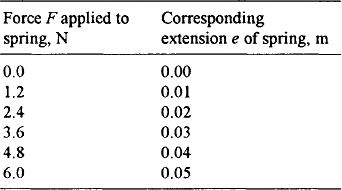
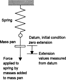
Figure 1.1 Simple spring with mass pan, the figure indicating the two physical quantities, namely the applied force and the resulting extension, that we are interested in determining the relationship between. Note, adding masses of 120 g results in force increments of about 1.2 N.
From Table 1.1, we can assume that there is some relationship or connection between the values of the force F acting on the spring and the corresponding observed extension e values. We can say:
Statement [1] is an inferred relationship between an observed measurement e and a varied quantity, in this case the applied force F. We can therefore call F the independent quantity, sometimes referred to as the argument, from which a dependent result is obtained. We can restate statement [1] as:
A function is a relationship which has for each value of the independent variable a unique value of the dependent variable. Statement [2] can be written as:
This means exactly the same thing as statement [2] but is just easier and more concise to write. The ‘f’ simply is shorthand for ‘function of’. Note that f(F) does not mean a variable f multiplied by F. When we are dealing with a number of different functions it is customary to use different letters for the function label, e.g. we might use y = f(x) and z = g(x).
With y = f(x) we have each value of y associated with an x value. We can plot such data points on a graph having x and y axes, the y-axis running vertically and the x-axis running horizontally and at 90° to the y-axis (Figure 1.2). The point of intersection of the two axes is called the origin; at this point y has the value 0 and x = 0. Values of x which are positive are plotted to the right of the origin, negative values to the left. Positive values of y are plotted upwards from the origin, negative values downwards.

Tables, graphs and equations to define functions
The statement e = f(F) merely tells us that the extension e is a function of the applied force F and does not describe the actual relationship between them. The data in Table 1.1 is one way we describe the relationship. If we know the force is 3.6 N then the extension must be 0.03 m.
However, a pattern can be seen from an inspection of the results in Table 1.1: if we double the applied force then the resulting extension doubles, if we treble the applied force the extension trebles and if we quadruple the applied force the extension quadruples. We can say, at least over the range of values we have observed:
and we can write this as:
The symbol ∝ simple means (or is shorthand for) ‘proportional to’.
We can also see how the extension depends on the applied force by plotting a graph. If we plot a graph of the force values in Table 1.1 against the corresponding extension values we obtain the straight line graph shown in Figure 1.3. The straight line passes through the origin. This is a characteristic of relationships when one quantity is directly proportional to the other. The graph is thus one way of defining the functional relationship.
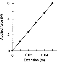
Figure 1.3 Force–extension graph for the spring experiment values given in Table 1.1
We can use the graph in Figure 1.3 to determine an equation relating the extension to the applied force and so give another way of defining the functional relationship. The graph is a straight line and so has a constant slope (or gradient), the slope being defined in the same way as we define the slope of a road, i.e. as the change in vertical height of the line over a given horizontal distance (Figure 1.4). We can compute the slope by choosing a pair of values of force and extension, e.g. force 60 N, extension 0.05 m; force 1.2 N, extension 0.01 m, and so obtain:
Since the straight line passes through the origin, this tells us that the force in newtons is, over the interval that has been considered, 120 times the extension in metres. We can write this as:
The constant term, i.e. the 120 N/m, is called the constant of proportionality linking F to the corresponding e values.

To summarise: we can define the functional relationship between two variables by:
• a set of results (as in Table 1.1),
• a graph (as in Figure 1.3),
• an equation (as in equation [4]).
Note that to define a function y = f(x) completely, we must define the range of values of x over which the definition is true. This is called the domain of the function.
Equations and functions
Functions may, as mentioned earlier, be defined using equations. Equations give the instructions for calculating the dependent variable of functions for values of the independent variable. For example, for an ohmic resistor the potential difference V across it is a function of the current I through it, i.e.
The equation defining the functional relationship (Ohm’s law) is V = RI, where R is the constant if proportionality connecting the variable V with the variable I, thereby defining their unique relationship. So given a value for the current we can use the equation to obtain a value of the potential difference. Thus, when R = 10 Ω and I = 2 A we have:
For an object freely falling from rest, the distance fallen s is a function of the time t for which it has been falling, i.e. s = f(t). The defining equation is s = ½at2, where a, the acceleration, is a constant. The acceleration is the acceleration due to gravity g and so we can write the defining equation as s = ½gt2. Thus, given a value for the time we can use the equation to obtain a value for the distance fallen. If we assume that g has a value of 9.8 m/s2, then for a time of 3 s;
Note that a function may be defined by several equations, with each giving the instructions for calculating the dependent variable for different values of the independent variable. For example, for the voltage signal shown in Figure 1.5, a so-called step voltage, we have v = f(t) and the relationship


The value of v = f(1) is thus 0, while the value of v = f(4) is 2 V.
Functions may of course get quite complex! For example, the natural frequency of transverse vibration of a cantilever is described by the equation:
The frequency of the cantilever is a function of E, I, m and L. So, in functional notation we can write:
1.1.1 Combinations of functions
Many of the functions encountered in engineering and science can be considered to be combinations of other functions. Suppose we have the function ![]() We can think of the function f(x) as resulting from the combination of two functions g(x) and h(x). One of the functions takes an input of x and gives an output of x2 and the other takes an input of x and gives an output of 2x. The two outputs are then added and we have f(x) = g(x) + h(x). Figure 1.6 illustrates this.
We can think of the function f(x) as resulting from the combination of two functions g(x) and h(x). One of the functions takes an input of x and gives an output of x2 and the other takes an input of x and gives an output of 2x. The two outputs are then added and we have f(x) = g(x) + h(x). Figure 1.6 illustrates this.

Another way we can combine functions is by applying them in sequence. For example, if we have h(x) = 2x and g(x) = x2, then suppose we have the arrangement shown in Figure 1.7. The input of x to the g function box results in an output of x2. The h function box takes its input and doubles it. Thus for an input of x2 we have an output of 2x2, thus f(x) = h{g(x)} = 2x2. Note that the order of the function boxes is important.

Problems 1.1
1. If we have y as a function of x and defined by the equation y = 2x + 3, what are the values of (a) f(0), (b) f(1)?
2. If we have y as a function of x and defined by the equation y = x2 + x, what are the values of (a) f(0), (b) f(2)?
3. If y is a function of x defined by the following equations, find the values of f(0) and f(1).
4. Determine the values of (a) f(0.5), (b) f(2) if we have y as a function of x and defined by:
5. Determine the values of (a) f(1) (b) f(3) if we have y as a function of t and defined by:
6. The voltage in an electrical circuit is supplied by a constant voltage source of 10 V. If the voltage is switched on after time t = 2 s, state the equations defining the step voltage at any time t.
7. Sketch the periodic waveform described by the following equations:
8. The period of oscillation T of a simple pendulum is a function of the length L of the pendulum, being defined by the equation
where g is the acceleration due to gravity. What are the values of (a) f(1), (b) f(10) if g can be taken as 10 m/s2?
9. The velocity v in metres per second of a moving object is a function of the time t in seconds, being defined by v = 2 + 5t. What are the values of (a) f(0), (b) f(1)?
10. If g(x) = 2x and h(x) = x + 1, what are (a) g(x) + h(x), (b) g{h(x)}, (c) h{g(x)}?
11. If f(x) = x2 + 1, g(x) = 3x and h(x) = 3x + 2, determine: (a) f(x) + g(x), (b) f{g(x)}, (c) g{f(x)}, (d) f(x) − h(x), (e) f{h(x)}.
1.2 Linear functions
This section is about a form of functions that is very commonly encountered in engineering, namely linear functions. Quite simply, linear functions are ones that provide a linear or straight line relationship between two variables when plotted as a conventional graph of one variable against the other.
The potential difference V across a resistor is a function of the current I through it. If the resistor obeys Ohm’s law then V = RI, the potential difference is proportional to the current. If the current is doubled then the potential difference is doubled, if the current is trebled the potential difference is trebled. This means that a graph of V plotted against I is a straight line graph passing through the origin. Gradient is defined as the change in y value divided by the change in x value. Thus, for all straight line graphs passing through the origin (Figure 1.8), the gradient is constant and given by gradient m = y/x. Hence the equation of such a straight line is of the form:
where m is the gradient of the line. Only when we have such a relationship is y directly proportional to x.

Figure 1.8 Straight line graph with y directly proportional to x; the straight line thus passes though the origin
Straight line graphs which do not pass through the origin (Figure 1.9) have a gradient, change in y value divided by change in x value, given by m = (y − c)/x, where c is the value of y when x = 0, i.e. the intercept of the straight line with the y-axis. Thus, such lines have the equation:
This is the equation which defines a straight line and is termed a linear equation. It is important to realise that with c ≠ 0 that y is not proportional to x.

The gradient m of a straight line graph may be positive or negative. The gradient may also have a value of zero and this is a line parallel to the x-axis. The intercept c may be positive or negative, or zero.
During a test to find how the power of a CNC lathe varied with depth of cut, the following results were obtained:
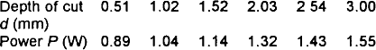
Use a graph to show that the function connecting the quantities d and P is of the form y = mx + c. Use this function to calculate the depth of cut when the power is 1 W.
Figure 1.10 shows the graph with P on the y-axis and d on the x-axis. The graph line represents the line of best fit through all the points and may therefore be prone to some error. Because it is a straight line, the function is of the form y = mx + c and so we have:
The slope m of the graph is about 0.27 and the point where the line would intercept the P axis when d = 0 is about 0.76. The function is thus:
We can check the integrity of the above equation by substituting values from the table of observed results, say d = 2.03 mm. This gives:
If we now refer back to the table of results we see that this is close to what is given there, i.e. 1.32 W.

To finally answer the question regarding the depth of cut to be expected when the power is 1 W:
Hence d is about 0.89 mm.
A pressure measurement system using a piezoelectric transducer is set up as represented by the system diagram of Figure 1.11. As the input pressure signal is altered, corresponding output readings are taken off the oscilloscope screen and the results shown below were obtained:

Use a graph to show that the function connecting the quantities output voltage θo to the pressure θi is of the form y = mx + c. The static sensitivity of such a measurement system may be defined as the change in output signal divided by the change in the corresponding input signal. Determine the static sensitivity.

Figure 1.12 shows the graph obtained by plotting the above values. The graph line represents the line of best fit through all the points and may therefore be prone to some error. Because it is a straight line, the function is of the form y = mx + c and so we have:
From the graph, the approximate slope m is 350/5.5 = 63.6 mV/bar. The line passes through the origin and so c = 0. Hence:
The symbol Δ in front of a quantity is used to indicate an increment of that quantity. But this is just the slope of the graph and so the static sensitivity is 63.6 mV/bar.

Problems 1.2
1. State which of the following will give a straight line graph and, if so, whether it passes through the origin:
(a) A graph of the extension of a spring plotted against the applied load when the extension is proportional to the applied load.
(b) A graph of the resistance R of a length of resistance wire plotted against the temperature t when R = R0(1 + at), with R0 and a being constants.
(c) A graph of the distance d travelled by a car plotted against time t when d = 10 + 4t2.
(d) A graph is plotted of the pressure p of a gas against its volume v, the pressure being related to the volume by Boyle’s law, i.e. pv = a constant.
2. Determine the straight line equations for the following data if linear functional relationships can be assumed:
1.3 Quadratic functions
A linear function is one where the equation defining the function is of the form y = mx + c. The highest power of a variable is 1. This is only one type of function. Here we look at another form, the quadratic function, and examine its defining equation.
The term quadratic function is used for a function y = f(x) where the defining equation has the general form:
where a, b and c are constants. The highest power of the variable is 2.
Quadratic equations occur often in engineering. An example of such an equation in engineering occurs with the e.m.f. E of a thermocouple which can often be described by:
where t is the temperature and a and b are constants. Other examples occur in the relationships for the bending moment M for bending beams, such as that for a cantilever propped at its free end:
where x is the distance from the free end of a cantilever of length L and w the distributed load per unit length.
The linear equation and the quadratic equation are just two examples of what are termed polynomials. A polynomial is the term used for any equation involving powers of the variable which are positive integers. Such powers can be 1, 2, 3, 4, 5, etc. For example, x4 + 4x3 + 2x2 + 5x + 2 = 0 is a polynomial with the highest power being 4.
1.3.1 Factors and roots
To factorise a number means to write it as the product of smaller numbers. Thus, for example, we can factor 12 to give 12 = 3 × 4. The 3 and 4 are factors of 12. If the 3 and the 4 are multiplied together then 12 is obtained. To factorise a polynomial means to write it as the product of simpler polynomials. Thus for the quadratic expression x2 + 5x + 6 we can write:
(x + 2) and (x + 3) are factors. If the two factors are multiplied together then the x2 + 5x + 6 is obtained. Note that, in general:
If we have u × v = 0 then we must have either u = 0 or v = 0 or both u and v are 0. This is because 0 times any number is 0. Thus if we have the quadratic equation x2 + 5x + 6 = 0 and rewrite it as (x + 2)(x + 3) = 0, then we must have either x + 2 = 0, or x + 3 = 0 or both equal to 0. This means that the solutions to the quadratic equation are the solutions of these two linear equations, i.e. x = −2 and x = −3. These values are called the roots of the equation. We can check these values by substituting them into the quadratic equation. Thus for x = −2 we have 4 − 10 + 6 = 0 and thus 0 = 0. For x = −3 we have 9 − 15 + 6 = 0 and thus 0 = 0.
Factorise and hence solve the quadratic equation x2 − 3x + 2 = 0.
To factorise this equation we need to find the two numbers which when multiplied together will give 2 and which when added together will give −3.
If we multiply −1 and −2 we obtain 2 and the addition of −1 and −2 gives −3. Thus we can write:
The solutions are thus given by x − 1 = 0, i.e. x = 1, and x − 2 = 0, i.e. x = 2.
We can check these values by substituting them into the original equation, x2 − 3x + 2. Thus, for x = 1 we have 1 − 3 + 2 = 0 and so 0 = 0. For x = 2 we have 4 − 6 + 2 = 0 and so 0 = 0.
The procedure for determining the roots of a quadratic equation by completing the square can be summarised as:
Completing the square
Consider the equation x2 + 6x + 9 = 0. This equation can be factorised to give (x + 3)(x + 3) = 0, i.e. (x + 3)2 = 0. It is a perfect square, both the roots being the same. Now consider the equation x2 + 6x + 2 = 0. What are the factors? We can rewrite the equation as:
If we add 9 to both sides of the equation then we obtain
The left-hand side of the equation has been made into a perfect square by the adding of the 9. Thus we can write:
This means that x + 3 must be one of the square roots of 7, i.e.
The plus or minus is because every positive number has two square roots, one positive and one negative. Thus we have ![]() Hence:
Hence:
The two solutions are thus ![]()
This method of determining the roots of a quadratic equation is known as completing the square. In the above discussion the left-hand side of the equation was made into a perfect square by the adding of 9. How do we determine what number to add in order to make a perfect square? Any expression of the form x2 + ax becomes a perfect square when we add (a/2)2, since:
Thus for x2 + 6x we have a = 6 and so (a/2) = 3; we add 32 = 9.
The above rule for completing the square only works if the coefficient of x2, i.e. the number in front of x2, is 1. However, if this is not the case we can simply divide throughout by that coefficient in order to make it 1.
Use the method of completing the square to solve the quadratic equation x2 + 10x − 4 = 0.
The quadratic equation can be written as:
Adding (10/2)2 = 25, to both sides of the equation gives:
Hence, x + 5 = ±√29 = ±5.39 and the solutions of the quadratic equation are x = +5.39 − 5 = 0.39 and x = −5.39 − 5 = −10.39.
We can check these values by substituting them in the equation x2 + 10x − 4 = 0. Thus, for x = 0.39 we have 0.392 + 3.9 − 4 = 0.05, which, because of the rounding used to limit the number of decimal places in determining the root, is effectively zero. For the other solution of x = −10.39 we have (−10.39)2 + 103.9 − 4 = 0.05, which, because of the rounding used to limit the number of decimal places in determining the root, is effectively zero.
The quadratic formula
Consider the quadratic equation ax2 + bx + c = 0. To obtain the roots by completing the square method, we divide throughout by a to give:
This can be written as:
To make the left-hand side of the equation a perfect square we must add (b/2a)2 to both sides of the equation. Hence:
and so:
Taking the square root of both sides of the equation gives
Thus:
and so we have the general formula for the solution of a quadratic equation:
Consider the following three situations:
• If we have (b2 − 4ac) > 0, then the square root is of a positive number. There are then two distinct roots which are said to be real.
• If we have (b2 − 4ac) = 0, then the square root is zero and the formula gives just one value for x. Since a quadratic equation must have two roots, we say that the equation has two coincident real roots.
• If we have (b2 − 4ac) < 0, then the square root is of a negative number. A new type of number has to be invented to enable such expressions to be solved. The number is referred to as a complex number and the roots are said to be imaginary (the roots in 1 and 2 above are said to be real). Such numbers are discussed later in this book.
Determine, if they exist as real roots, the roots of the following quadratic equations:
(a) Using the general quadratic formula [10], here we have a = 4, b = −7 and c = 3. Therefore:
Therefore, x = 1 or x = 0.75 defines the two roots of the equation. We can now represent the function as:
and this, when multiplied out, gives x2 − 1.75x + 0.76 and which when multiplied by 4 gives the original equation 4x2 − 7x + 3.
(b) Using the general quadratic formula [10] gives:
Therefore, we have two roots with x = 2. We may now rewrite the equation in the form (x − 2)(x − 2). This, when multiplied out, gives x2 − 4x + 4.
(c) Using the general quadratic formula [10] gives:
Since the term inside the square root is negative, we have no real roots.
Figure 1.13 shows a simple cantilever of length L, propped at its free end. It can be shown that the bending moment M of this type of cantilever is a function of the distance x measured from the fixed end of the beam, thus M = f(x). The defining equation for the function is:
where W is the distributed load in newtons per unit length. Using this quadratic formula, determine the positions along the beam at which the bending moment is zero (in engineering called the points of contraflexure).

We can solve this by using the general quadratic formula [10]. Firstly, we can simplify the expression by multiplying through by 8 and taking the W term out as a factor:
and so the equation becomes 4x2 − 5Lx + L2 = 0. Thus:

Hence x = L/4 or x = L. The bending moment is thus zero at two locations (it has two points of contraflexure), i.e. at L/4 from the fixed end or at the extreme right-hand end of the beam when x = L.
The distance s in metres moved by a vehicle over a period of time t seconds is defined by the equation s = ut + ½at2, with a being the constant acceleration and u the initial velocity. Assuming the vehicle commences motion with an initial velocity of 5 m/s and covers 84 m with a constant acceleration of 2 m/s2, calculate the time over which this occurs.
Substituting the values in the equation gives:

Writing the equation in the general format:
Thus:
and so t = −12 s or t = 7 s. Since we cannot have a negative time, the only acceptable answer is t = 7 s.
The solution may be checked by substituting into the original equation t2 + 5t − 84 = 0, when t = 7 s we have 72 + 5(7) − 84 = 0. Since this is true, our solution holds.
The total surface area A of a cylinder of radius r and height h is given by the equation A = 2πr2 + 2πrh. If h = 6 cm, what will be the radius required to give a surface area of 88/7 cm2? Take π as 22/7.
Putting the numbers in the equation gives
Multiplying throughout by 7 and dividing by 44 gives
Hence we can write
and so:
Hence the solutions are r = −6.32 cm and r = 0.32 cm. The negative solution has no physical significance. Hence the solution is a radius of 0.32 cm.
We can check this value of 0.32 cm by substitution in the equation 2 = r2 + 6r. Hence 0.10 + 1.92 = 2.02, which is effectively 2 bearing in mind the rounding of the root value to two decimal places that has occurred.
Problems 1.3
1. Determine, if they exist, the real roots of the following quadratic functions:
2. The e.m.f. E of a thermocouple is a function of the temperature T, being given by E = −0.02T2 + 6T. The e.m.f. is in μV and the temperature in °C. Determine the temperatures at which the e.m.f. will be 200 μV
3. When a ball is thrown vertically upwards with an initial velocity u from an initial height ho, the height h of the ball is a function of the time t, being given by h − h0 = ut − 4.9t2. Determine the times for which the height is 1 m, if u = 4 m/s and h0 = 0.5 m.
4. The deflection y of a simply supported beam of length L when subject to an impact load of mg dropped from a height h on its centre is obtained by equating the total energy released by the falling load with the strain energy acquired, i.e.
Hence obtain an expression for the deflection y.
5. The height h risen by an object, after a time t, when thrown vertically upwards with an initial velocity u is given by the equation ![]() where g is the acceleration due to gravity. Solve the quadratic equation for t if u = 100 m/s, h = 150 m and g = 9.81 m/s2.
where g is the acceleration due to gravity. Solve the quadratic equation for t if u = 100 m/s, h = 150 m and g = 9.81 m/s2.
6. A rectangle has one side 3 cm longer than the other. What will be the dimensions of the rectangle if the diagonals have to have lengths of 10 cm? Hint: let one of the sides have a length x, then the other side has a length of 3 + x. The Pythagoras theorem can then be used.
1.4 Inverse functions
So far, in the treatment of a function we have started with a value of the independent variable x and used the function to find the corresponding value of the dependent variable y (Figure 1.14(a)). However, suppose we are given a value for y and want to find x (Figure 1.14(b)). For example, we might have distance s as a function of time t, e.g. s = 2t. Given a value of the independent variable t we can use the function to determine s. Suppose though that we are given a value of the dependent variable s and have to determine the corresponding t value? With the given equation we can rearrange it to give t = s/2. The function from t to s is f(t), the function from s to t is a different function g(s).

Figure 1.15(a) shows some values for the s = f(t) function described by the equation s = 2t. Figure 1.15(b) shows the function obtained by reversing the arrows, i.e. starting with time values deducing the corresponding distance values. This figure represents the inverse relationship.

Note that there is a simple point of significance here: if we use s = 2t to calculate a value for s given a value of t and then use the inverse by taking that value of t to calculate a value of s, we end up back where we started with our original value of s. This leads to a method of specifying an inverse function. Consider the arrangement shown in Figure 1.16. Here the g function system box operates on the output from the f function box in order to undo the work of the f box. Because the g function is undoing the work of the f function it is said to be the inverse of f. We may, therefore, write:
This equation [11] is used to define an inverse function:
If f is a function of x then the function g which satisfies g{f(x)}= x for all values of x in the domain of f is called the inverse off.
With regard to notation: the inverse of a function f of x is written as f−1(x). Note that f−1(x) does not mean 1/f(x), it is simply the notation to indicate the inverse function (the −1 not indicating a a power −1!). f−1(x) takes an input which is some function of x and inverts it to give an output of x. Thus the above definition gives:
As an illustration, consider a function f which adds 2, i.e. we have f(x) = x + 2 (Figure 1.17(a)). Then the inverse is a function that subtracts 2 in order to undo the action of the f function (Figure 1.17(b)). Thus, f−1(x) = x − 2 and so if we put into the function x + 2 we obtain (x + 2) − 2.

As a further illustration, consider a function f which multiplies by 3, i.e. we have f(x) = 3x (Figure 1.18(a)). Then the inverse is a function that divides by 3 in order to undo the action of the f function (Figure 1.18(b)). Thus f−1(x) = x/3.

As another illustration, consider a function which multiplies by 3 and then adds 2, i.e. f(x) = 3x + 2. Here we have operated on the input x to the function twice, initially we multiplied the x by 3 and then we added the number 2 (Figure 1.19(a)). To arrive back at the original input, the inverse do two things (the reverse operation of those just detailed), namely initially subtract 2 and then secondly divided through by 3 (Figure 1.19(b)). Note that you must undo things in the reverse order to which they were done with the function f.

Figure 1.19 (a) The functions which multiply by 3 and then add 2, (b) the inverse functions which subtract 2 and then divide by 3
The above illustrations are rather basic functions. We will investigate more complex ones later. However, the basic rules still apply and, once understood, will provide a solid foundation from which to build more complex relationships.
1.4.1 Graphs of f and f−1
We can use the above rules for a function and its inverse to find the graph of an inverse function from a graph of the function. Consider the graph of y = f(x) shown in Figure 1.20(a). This is the graph described by the equation y = x2. What is the graph of the inverse function f−1(x)? This will be the graph of y = √x (Figure 1.20(b)) since the function √x is what we need to apply to undo the function x2.

If we examine the two graphs we find that the inverse f−1 is just the reflection of the graph of f in the line y = x (Figure 1.21). This is true for any function when it possesses an inverse.

1.5 Circular functions
This section focuses on the so-called circular or trigonometric functions. Such functions are widely used in engineering. Thus in describing oscillations, whether mechanical of perhaps a vibrating beam or electrical and alternating current, the equations used to define the quantity which fluctuates with time is likely to involve a trigonometric function.
As an illustration, consider the mechanical oscillation of a mass on the end of a spring when is just vibrates up-and-down when the mass is given a vertical displacement (Figure 1.22). With very little damping, the mass will oscillate up-and-down for quite some time. Figure 1.23 shows how the displacement varies with time.


Figure 1.23 Displacement y variation with time for the oscillating mass when damping is virtually absent
If we look at the situation when there is noticeable damping present, then the displacement variation with time looks more like Figure 1.24. The difference between this graph and Figure 1.23 is that, though we have a similar form of graph, the effect of the damping is that the amplitude decreases with time.
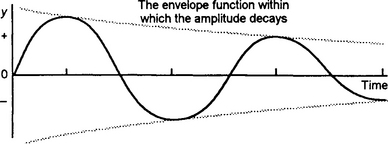
We can derive an equation to represent the variation of displacement with time in the absence of damping by using a simple model. Suppose we draw a circle with a radius OA equal to the amplitude of the oscillation, i.e. the maximum displacement, and consider a point P moving round the circle with a constant angular velocity ω (Figure 1.25) and starting from the horizontal. The vertical projection of the rotating radius OP gives a displacement-angle graph. Since the radius OP is rotating with a constant angular velocity, the angle rotated is proportional to the time. The result is a graph which replicates that of the undamped oscillating mass.

The convention used for angles is that they are referenced from zero degrees and when measured in an anticlockwise direction are termed positive angles. One unit for angles is degrees (Figure 1.26(a)). However, when angles occur in equations in engineering, it is usual to describe them in radians. One complete rotation of a radius is a rotation through 360°.
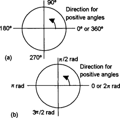
One radian is the angle swept so that the arc formed is the same length as the radius, hence since one complete sweep of a radius is an arc length of 2πr, then one complete rotation is 2π radians (Figure 1.26(b)). Thus 360° = 2π radians (rad) and so 1 rad = 360/2π = 57.3°.
Since AB/OA = sin θ we can write:
where AB is the vertical height of the line at some instant of time, OA being its length. The maximum value of AB will be OA and occur when θ = 90°. But a constant angular velocity ω means that in a time t the angle θ covered is ωt. Thus the vertical projection AB of the rotating line will vary with time and is described by the equation:
If y is the displacement of the alternating mass and A the amplitude of its oscillation, the equation can be written as:
This type of oscillation is called simple harmonic motion.
It is usual to give angular velocities in units of radians per second, an angular rotation through 360° being a rotation through 2π radians. Since the periodic time T is the time taken for one cycle of a waveform, then T is the time taken for OA to complete one revolution, i.e. 2π radians. Thus:
The frequency f is 1/T and so ω = 2πf. Because ω is just 2π times the frequency, it is often called the angular frequency. The frequency f has units of hertz (Hz) or cycles per second and thus the angular frequency has units of s−1. We can thus write the above equation as:
We can use a similar model to describe alternating current; in this case the rotating radius OP is called a phasor. Thus the current i is related to its maximum value I by:
For the damped oscillation, the amplitude decreases with time so we must figure out how to quantify this ‘decay’ and link it somehow with the basic sine wave function of the undamped system. As we will later discover, the damped oscillation is actually described by a combination of a sine function and an exponential function.
The definitions used to define the trigonometric ratios in terms of a right-angled triangle (Figure 1.28) are:

The circular functions
We can define the circular functions, i.e. the sine, cosine and tangent, in terms of the rotation of a radial arm of length A (it often represents the amplitude) in a circular path (Figure 1.27). Thus, we can define the sine of an angle as:

But, with b = yi − 0, then sin θ = y1/A and so:
This relationship now enables us to calculate the vertical side of the triangle Ox1P, or the y-coordinate of point P.
Likewise, we can define the cosine of an angle as:
But, with c = x1 − 0, then cos θ = x1/A and so:
This relationship now enables us to calculate the horizontal side of the triangle Ox1P, or the x-coordinate of point P.
We can define the tangent of an angle in terms of the gradient of the line OP as:
Using equations [15] and [16] we can write equation [17] as:
With reference to Figure 1.27, as the point P moves around the circle, so the angle θ changes. The trigonometrical ratios can be defined in terms of the angles in a right-angled triangle. However, the above definitions allow us to define them for all angles, not just those which are 90° or less. Because they are defined in terms of a circle, they are termed circular functions.
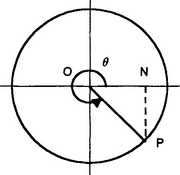
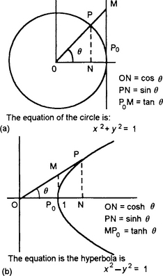
Consider the motion of a point P around a unit radius circle (Figure 1.29). P0 is the initial position of the point and P the position to which it has rotated. The radial arm OP in moving from OP0 has swept out an angle θ. The angle θ is measured between the radial arm and the OP0 axis as a positive angle when the arm rotates in an anticlockwise direction. Since the circle has a unit radius, to obtain for angles up to 90° the same result as the trigonometric ratios defined in terms of the right-angled triangle, the perpendicular height NP defines the sine of the angle P0OP and the horizontal distance ON defines the cosine of the angle P0OP.

Consider the circular rotations for angles in each quadrant (note: the first quadrant is angles 0° to 90°, the second quadrant 90° to 180°, the third quadrant 180° to 270°, the fourth quadrant 270° to 360°):
When the radial arm OP is in the first quadrant (Figure 1.30) with 0 ≤ θ < π/2, 0 ≤ θ < 90°, both NP and ON are positive. Thus both the sine and the cosine of angle θ are positive. Since the tangent is NP/ON then the tangent of angle θ is positive. For example, sin 30° = +0.5, cos 30° = +0.87 and tan 30° = +0.58.

2. Angles between 90° and 180°
When the radial arm OP moves into the second quadrant (Figure 1.31) with π/2 ≤ θ < π, 90° ≤ θ < 180°, NP is positive and ON negative. Thus the sine of angle θ is positive and the cosine negative. Since the tangent is NP/ON then the tangent of angle θ is negative. For example, sin 120° = 0.87, cos 120° = −0.50 and tan 120° = −1.73.

3. Angles between 180° and 270°
When the radial arm moves into the third quadrant (Figure 1.32) with π ≤ θ < 3π/2, 180° ≤ θ < 270°, NP is negative and ON negative. Thus the sine of angle θ is negative and the cosine negative. Since the tangent is NP/ON then the tangent of angle θ is positive. For example, sin 210° = −0.5, cos 210° = −0.87 and tan 210° = +0.58.

4. Angles between 270° and 360°
When the radial arm is in the fourth quarter (Figure 1.33) with 3π/2 ≤ θ < 2π, 270° ≤ θ < 360°, NP is negative and ON positive. Thus the sine of angle θ is negative and the cosine positive. Since the tangent is NP/ON then the tangent of angle θ is negative. For example, sin 300° = −0.87, cos 300° = 0.5 and tan 300° = −1.73.
We can now summarise with Figure 1.34 as an aid to memory.

For angles greater than 2π rad (360°), the radial arm OP simply rotates more than one revolution. Negative angles are interpreted as a clockwise movement of the radial arm from OP0.
Cyclic functions
A cyclic function is one which repeats itself on a cyclic period. Thus, if we have a function y = f(x) which is cyclic and repeats itself after a time T, then:
T is termed the periodic time and is the time taken to complete one cycle. Hence, if the frequency is f then f cycles are completed each second and so T = 1/f.
As the arm OP in Figure 1.35 rotates round-and-round its circular path, the values of its vertical projection NP is cyclic and generates the sine graph shown. Since the graph describes a periodic function of period 2π, then:
where n = 0, ±1, ±2, etc.

Note that if OP rotates in a clockwise direction, i.e. the negative direction, then as θ is negative, this generates the sine function continued to the left of the origin O into the negative region (Figure 1.36). For negative values of θ, the sine function has the same values as the positive values except for a change in sign:
To obtain the graph of cos θ as the radial arm OP rotates round-and-round its circular path, we read off the values of its horizontal projection ON. Figure 1.37 shows the result. Since the graph describes a periodic function of period 2π, then:


where n = 0, ±1, ±2, etc.
Note that the graph of y = sin θ is the same as that of y = cos θ moved ½π to the right, while that of y = cos θ is the same as y = sin θ moved ½π to the left, i.e. sin θ = cos (θ − ½π) and cos θ = sin (θ + ½π).
In the projections of the radial arm OP to generate the sine or cosine graphs, we have let OP have the value of 1. If we consider a radial arm of length A, we have the same function but multiplied by A, i.e. y = A sin θ. The amplitude of the waveform is changed. To illustrate this look at the following functions and their graphs as plotted to the same scale and on the same axes (Figure 1.38): y = 1 sin θ with amplitude A = 1, y = 4 sin θ with amplitude A = 4 and y = 0.5 sin θ with amplitude A = 0.5.

In engineering, we often encounter functions of the general form:
φ is the initial angle we start the rotating radial arm OP at and, as a consequence, φ is the angle by which the sine or cosine graph is moved to the left when positive and to the right when negative. It defines a phase shift of the complete waveform. Figure 1.39 illustrates this by showing the effect of a phase shift of π/3, i.e. 60°.
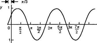
Figure 1.39 Graph of y = sin (θ + π/3), showing the effect of a phase shift of π/3, i.e. 60°, as being to shift the graph to the left by that amount
Now consider the graph of the function y = tan x. For the radial arm OP rotating in a circle, the tangent is PN/OP (Figure 1.40). But if we draw a tangent to the circle at Po then, for a unit radius circle the tangent of the angle is P0M. When the radius arm has moved to an angle between 90° and 180° then the tangent is P0M1. The graph describes a periodic function which repeats itself every period of π (not every 2π as for a sine or cosine function). Thus:
for n = 0, ±1, ±2, etc.

Draw graphs of y = cos θ and y = cos 2θ on the same axis and comment on how they differ.
A simple way to sketch the graphs is to formulate a table for values between θ = 0° and θ = 360° for cos θ and cos 2θ, then plot the respective curves. So we have:

Figure 1.41 shows the resulting graphs.

Sketch the function y = 5 sin (θ + 30°) for values of θ between 0° and 360°.
The equation indicates that the waveform has an amplitude of 5 and a phase shift of +30°. Figure 1.42 shows the form of the function.

To illustrate a simple mechanical application, consider a piston head moving cyclically without damping, i.e. without friction, and represented by the spring-mass system shown in Figure 1.43. The spring represents the restoring or elastic driving force acting on the piston head.

We can find some basic properties of the system if we apply cyclic functions. We assume that the motion can be represented by the y-component of a rotating radial arm which rotates with a constant angular velocity and so is given by y = A sin θ, where y is the vertical displacement at a time t. Since θ = ωt, we can write:
From mechanical theory, the angular frequency ω is:
where k is the spring constant and m the mass. Hence ω = √(144/4) = 6 rad/s and so y = A sin 6t. We thus have y at a maximum when sin 6t = 1, i.e. when 6t = 1.57 and so t = 0.26 s.
If the maximum displacement, i.e. amplitude, of the piston is 0.1 m, we have y = 0.1 sin 6t. Thus, at t = 3 s we have y = 0.1 sin 6(3) = 0.1 sin 18 = 0.1. Since 18 rad = 1031° then y = 0.1 (−0.75) = −0.075 m. The minus sign indicates that the displacement is in the upward direction from the datum line.
Phasors
A sinusoidal alternating current can be represented by the equation i = I sin ωt, where i is the current at time t and I the maximum current. In a similar way we can write for a sinusoidal alternating voltage v = V sin ωt, where v is the voltage at time t and V the maximum voltage. Thus we can think of an alternating current and voltage in terms of a model in which the instantaneous value of the current or voltage is represented by the vertical projection of a line rotating in an anticlockwise direction with a constant angular velocity. The term phasor, being an abbreviation of the term phase vector, is used for such rotating lines. The length of the phasor can represent the maximum value of the sinusoidal waveform (or the generally more convenient root-mean-square value, the maximum value is proportional to the root-mean-square value). The line representing a phasor is drawn with an arrowhead at the end that rotates and is drawn in its position at time t = 0, i.e. the phasor represents a frozen view of the rotating line at one instant of time of t = 0 (Figure 1.44).
Alternating currents or voltages which do not always start with zero values at time t = 0 and can be represented in general by:
The phasor for such alternating currents or voltages is represented by a phasor (Figure 1.45) at an angle φ to the reference line, this line being generally taken as being the horizontal. The angle φ is termed the phase angle. We can describe such a phasor by merely stating its magnitude and phase angle (the term used is polar coordinates). Thus ![]() A describes a phasor with a magnitude, represented by its length, of 2 A and with a phase angle of 40°.
A describes a phasor with a magnitude, represented by its length, of 2 A and with a phase angle of 40°.

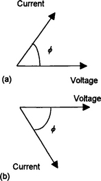
In discussing alternating current circuits we often have to consider the relationship between an alternating current through a component and the alternating voltage across it. If we take the alternating voltage as the reference and consider it to be represented by a horizontal voltage phasor, then the current may have some value at that time and so be represented by another phasor at some angle φ. There is said to be a phase difference of φ between the current and the voltage. If φ has a positive value then the current is said to be leading the voltage, if a negative value then lagging the voltage (Figure 1.46).
A sinusoidal voltage has a maximum value of 10 V and a frequency of 100 Hz. If the voltage has a phase angle of 30°, what will be the instantaneous voltage at times of (a) t = 0, (b) t = 0.5 ms?
The equation for the sinusoidal voltage will be:
The term 2πft, i.e. ωt, is in radians. Thus, for consistency, we should express φ in radians. An angle of 30° is π/6 radians. Thus:
It should be noted that it is quite common in engineering to mix the units of radians and degrees in such expressions. Thus you might see:
However, when carrying out calculations involving the terms in the bracket there must be consistency of the units.
1.5.2 Manipulating circular functions
Often in working through engineering problems, it is necessary to rearrange circular functions in a different format. This section looks at how we can do this.
The cosecant, secant and cotangent ratios are defined as the reciprocals of the sine, cosine and tangent:


Trigonometric relationships
For the right-angled triangle shown in Figure 1.47, the Pythagoras theorem gives AB2 + BC2 = AC2. Dividing both sides of the equation by AC2 gives:

Dividing this equation by cos2 θ gives:
and dividing equation [25] by sin2 θ gives:

Trigonometric ratios of sums of angles
It is often useful to express the trigonometric ratios of angles such as A + B or A − B in terms of the trigonometric ratios of A and B. In such situations the relationships shown in Key points prove useful.
As an illustration of how we can derive such relationships, consider the two right-angled triangles OPQ and OQR shown in Figure 1.48:

If we replace B by −B we obtain:
If in equation [28] we replace A by (π/2 − A) we obtain:
If in equation [29] we replace B by −B we obtain:
We can obtain tan (A + B) by dividing sin (A + B) by cos (A + B) and likewise tan (A − B) by dividing sin (A − B) by cos (A − B). By adding or subtracting equations from above we obtain the relationships such as 2 sin A cos B.
If, in the above relationships for the sums of angles A and B we let B = A we obtain the double-angle equations shown in Key points.

Solve the equation cos 2x + 3 sin x = 2.
Using equation [46] for cos 2x gives:

Hence sin x = ½ or 1. For angles between 0° and 90°, x = 30° or 90°.


Sometimes it is useful to write an equation of the form a sin θ + b cos θ in the form R sin (θ − a). We can do this by using the trigonometric formula for compound angles, e.g. equation [29] for sin (A − B). Thus:
Therefore, comparing coefficients of the sin θ terms:
and comparing coefficients of the cos θ terms:
Dividing these two equations gives
This leads us to be able to describe the angle a by the right-angled triangle shown in Figure 1.49. Hence:

The Key points show other relationships which can be derived in a similar way.
Express 3 cos θ + 4 sin θ in the form (a) R cos (θ − a), (b) R sin (θ + a).
(a) We can derive it by using the double-angle formula cos (A − B) = cos A cos B + sin A sin B. Thus:
Thus 3 = R cos a and 4 = R sin a. Hence tan a = 4/3 and so a = 53.1° or 0.93 rad. R = √(32 + 42) = 5. Hence:
(b) We can derive it by directly using the double-angle relationship sin (A + B) = sin A cos B + cos A sin B. Thus:
Thus 3 = R sin a and 4 = R cos a. Hence tan a = 3/4 and so a = 36.9° or 0.64 rad. R − √(32 + 42) = 5. Hence:
Express 6 sin ωt − 2.5 cos ωt in the form R sin (ωt + a).
Using the double angle formula sin (A + B) = sin A cos B + cos A sin B:
Comparing coefficients of sin ωt gives 6 = R cos a and of cos ωt gives −2.5 = R sin a. Thus tan a = −2.5/6. The negative sign for the sine and the tangent means that the angle must be in the fourth quadrant (see Figure 1.34). Hence a = −0.39 rad. R = √(62 + 2.52) = 6.5 and so:
Thus, by subtracting the waveform 2.5 cos ωt from 6 sin ωt we end up with a waveform of amplitude 6.5 and a phase shift of −0.39 rad.
Adding phasors
Often in alternating current circuits we need to add the voltages across two components in series. We must take account of the possibility that the two voltages may not be in phase, despite having the same frequency since they are supplied by the same source. This means that if we consider the phasors, they will rotate with the same angular velocity but may have different lengths and start with a phase angle between them. Consider one of the voltages to have an amplitude V1 and zero phase angle (Figure 1.50(a)) and the other an amplitude V2 and a phase difference of φ from the first voltage (Figure 1.50 (b)). We can obtain the sum of the two by adding the two graphs, point-by-point, to obtain the result shown in Figure 1.50(c). Thus at the instant of time indicated in the figures, the two voltages are v1 and v2. Hence the total voltage is v = v1 + v2. We can repeat this for each instant of time and hence end up with the graph shown in Figure 1.50(c).

However, exactly the same result is obtained by adding the two phasors by means of the parallelogram rule of vectors. If we place the tails of the arrows representing the two phasors together and complete a parallelogram, then the diagonal of that parallelogram drawn from the junction of the two tails represents the sum of the two phasors. Figure 17.16(c) shows such a parallelogram and the resulting phasor with magnitude V.
If the phase angle between the two phasors of sizes V1 and V2 is 90°, as in Figure 1.51, then the resultant can be calculated by the use of the Pythagoras theorem as having a size V of:

and is at a phase angle φ relative to the phasor for V2 of:
Two sinusoidal alternating voltages are described by the equations of v1 = 10 sin ωt volts and v2 = 15 sin (ωt + π/2) volts. Determine the sum of these voltages.
Figure 1.52 shows the phasor diagram for the two voltages. The angle between the phasors is π/2, i.e. 90°. We could determine the sum from a scale drawing or by calculation using the Pythagoras theorem. Thus:
Hence the magnitude of the sum of the two voltages is 18.0 V. The phase angle is given by:

Hence φ = 56.3° or 0.983 rad. Thus the sum is an alternating voltage described by a phasor of amplitude 18.0 V and phase angle 56.3° (or 0.983 rad). This alternating voltage is thus described by:
1.5.4 The inverse circular functions
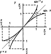
If sin x = 0.8 what is the value of x? This requires the inverse being obtained. There is an inverse if the function is one-to-one or restrictions imposed to give this state of affairs. However, the function y = sin x gives many values of x for the same value of y. To obtain an inverse we have to restrict the domain of the function to −π/2 to +π/2. With that restriction y = sin x has an inverse. The inverse function is denoted as sin−1 x (sometimes also written as arcsin x). Note that the −1 is not a power here but purely notation to indicate the inverse. If sin x = 0.8 then the value of x that gives this sine is the inverse and so x = sin−1 0.8, i.e. x = 53°. Figure 1.53 shows the graphs for sin x and its inverse function. In a similar way we can define inverses for cosines and tangents.
Problems 1.5
1. State the amplitude and phase angle (with respect to y = 5 sin θ) of the function y = 5 sin (θ + 30°).
2. A cyclic function used to describe a rotating radius (phasor) is defined by the equation y = 4 sin 3t. What is the amplitude and the angular frequency of the function?
3. State the amplitude, period and phase angle for the following cyclic functions:
4. State the amplitude, period and phase angle for the following cyclic functions:
5. The potential difference across a component in an electrical circuit is given by the equation v = 40 sin 40πt. Deduce the maximum value of the potential difference and its frequency.
6. A sinusoidal voltage has a maximum value of 1 V and a frequency of 1 kHz. If the voltage has a phase angle of 60°, what will be the instantaneous voltage at times of
7. A sinusoidal alternating current has an instantaneous value i at a time t, in seconds, given by i = 100 sin (200πt − 0.25) mA. Determine (a) the maximum current, (b) the frequency, (c) the phase angle.
8. A sinusoidal alternating voltage has an instantaneous value v at a time t, in seconds, given by v = 12 sin (100πt + 0.5) volts. Determine (a) the maximum voltage, (b) the frequency, (c) the phase angle.
9. What is the value of v, when t = 30 μs, for an amplitude-modulated radio wave with a voltage v in volts which varies with time t in seconds and is defined by the equation v = 50(1 + 0.02 sin 2400πt) sin (200 × 103πt).
10. Show that sin (A + B + C) = cos A cos B cos C (tan A + tan B + tan C − tan A tan B tan C).
11. Find the values of x between 0 and 360° which satisfy the condition 8 cos x + 9 sin x = 7.25.
12. Write 5 sin θ + 4 cos θ in the forms (a) R sin (θ − α), (b) R cos (θ + α).
13. Express W (sin α + μ cos α) in the form R cos (α − β) giving the values of R and tan β. Also show that the maximum value of the expression is W√(1 + μ2) and that this occurs when tan α = 1/μ.
14. Write the following functions in the form R sin (ωt + α):
15. Express 3 sin θ + 5 cos θ in the form R sin (θ + α) with α measured in degrees.
16. Write the following functions in the form R sin (ωt ± a):
17. The currents in two parallel branches of a circuit are 10 sin ωt milliamps and 20 sin (ωt + π/2) milliamps. What is the total current entering the parallel arrangement?
18. The voltage across a component in a circuit is 5.0 sin ωt volts and across another component in series with it 2.0 sin (ωt + π/6) volts. Determine the total voltage across both components.
19. The sinusoidal alternating voltage across a component in a circuit is 50√2 sin (ωt + 40°) volts and across another component in series with it 100√2 sin (ωt − 30°) volts. What is the total voltage across the two components?
20. The currents in two parallel branches of a circuit are 4√2 sin ωt amps and 6√2 sin (ωt − π/3) amps. What is the total current entering the parallel arrangement?
1.6 Exponential functions
There are many situations in engineering where we are concerned with functions which grow or decay with time, e.g.
• The variation with time of the temperature of a cooling object.
• The variation with time of the charge on a capacitor when it is being charged and when it is being discharged.
• The variation with time of the current in a circuit containing inductance when the current is first switched on and then when it is switched off.
• The decay with time of the radioactivity of a radioactive isotope.
This section is about the equations we can use to describe such growth or decay.
Exponentials
In general, we can describe growth and decay processes by an equation of the form:
where a is some constant called the base, and y the value of the quantity at a time t. Thus, for growth, we might have 2t, 3t, 4t, etc. and for decay 2−t, 3−t, 4−t, etc. We could write equations for growth or decay processes with different values of the base. However, we usually standardise the base to one particular value. The most widely used form of equation is ex, where e is a constant with the value 2.728 281 828 … Whenever an engineer refers to an exponential change he or she is almost invariably referring to an equation written in terms of ex. Why choose this strange number 2.718… for the base? The reason is linked to the properties of expressions written in this way. For y = ex, the rate of change of y with x, i.e. the slope of a graph of y against x, is equal to ex (this is discussed in more detail in the chapter concerned with differentiation):
and there are many engineering situations where this property occurs.
A simple illustration of the above is given if we take a strip of paper and cut it into half, throwing away one of the halves. We then take the half strip and cut it into half, throwing away one of the halves. If we keep on repeating this procedure we obtain the graph shown in Figure 1.54(a). This is an exponential decay in the length of the paper. Now look at the change in length per tear, i.e. the ‘gradient’ of the graph, Figure 1.54(b). We have the same exponential function. A similar type of relationship exists in the discharge of a charged capacitor. The charge on the capacitor decreases exponentially with time and the rate of change of charge, i.e. the current, follows the same exponential decay.

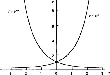
The following shows the values of ex and e−x for various values of x and Figure 1.55 the resulting graphs
![]()
![]()
The ex graph describes a growth curve, the e−x a decay curve. Note that both graphs have y = 1 when x = 0.
In a more general form we can write the exponential equation in the form y = ekx, or y = e−kx, where k is some constant. This constant k determines how fast y changes with x. The following data illustrates this:


The bigger k is the faster y decreases, or increases, with x.
When x = 0 then for y = ekx, or y = e−kx, y = e0 and so y = 1. This is thus the value of y that occurs when x is zero. Since we may often have an initial value other than 1, we write the equation in the form:
where A is the initial value of y at x = 0. For example, for the discharging of a capacitor in an electrical circuit we have, for the charge q on the capacitor at a time t, the equation:
When t = 0 then q = Q0. The constant k is 1/CR. The bigger the value of CR the smaller the value of 1/CR and so the slower the rate at which the capacitor becomes discharged.
One form of equation involving exponentials that is quite common is of the form:
When x = 0 then e0 = 1 and so y = A − A = 0. The initial value is thus 0. As x increases then e−kx decreases from 1 towards 0, eventually becoming zero when x is infinite. Thus the value of y increases as x increases. When x is very large then e−kx becomes virtually 0 and so y becomes equal to A. Figure 8.4 shows the graph. It shows a quantity y which increases rapidly at first and then slows down to become eventually A.

For example, for a capacitor which starts with zero charge on its plates and is then charged we have the equation:
When t = 0 then e0 = 1 and so q = Q0 − Q0 = 0. As t increases, so the value of e−t/CR decreases and so q becomes more and more equal to Q0.
Consider the discharging of a charged capacitor through a resistance (Figure 1.57). The voltage vC across the capacitor varies with time t according to the equation vC = V e−RC, where V is the initial potential difference across the capacitor at time t = 0. Suppose we let τ = RC, calling τ the time constant for the circuit. Thus, vC = V e−t/τ. The time taken for vC to drop from V to 0.5V is thus given by:
Thus in a time of 0.693τ the voltage will drop to half its initial voltage. The time taken to drop to 0.25V is given by:


Thus in a time of 1.386τ the voltage will drop to one-quarter of its initial voltage. This is twice the time taken to drop to half the voltage. This is a characteristic of a decaying exponential graph: if t is the time taken to reach half the steady-state value, then in 2t it will reach one-quarter, in 3t it will reach one-eighth, etc. In each of these time intervals it reduces its value by a half (Figure 1.58).

When t = 1τ then vC = V e−1 = 0.632V. Thus in a time equal to the time constant the voltage across the capacitor drops to 63.2% of the initial voltage. When t = 2x then vC = V e−2 = 0.135V. Thus the voltage across the capacitor drops to 13.5% of the initial voltage. When t = 3τ then vC = V e−3 = 0.050V. Thus the voltage across the capacitor drops to 5.0% of the initial voltage.
Now consider the growth of the charge on an initially uncharged capacitor when a voltage is switched across it (Figure 1.59). The time constant τ is RC. Thus:
What time will be required for vC to reach 0.5V?

Thus in a time of 0.693τ the voltage will reach half its steady-state voltage. The time taken to reach 0.75V is given by:

Thus in a time of 1.386τ the voltage will reach three-quarters of its steady-state value. This is twice the time taken to reach half the steady-state voltage. This is a characteristic of exponential graphs: if t is the time taken to reach half the steady-state value, then in 2t it will reach three-quarters, in 3t it will reach seven-eighths, etc. In each successive time interval of 0.7τ the p.d. across the capacitor reduces its value by a half (Figure 1.60).

When t = 1τ then vC = 1/(1 − e−1) = 0.632V. Thus in a time equal to the time constant the voltage across the capacitor rises to 63.2% of the steady-state voltage. When t = 2τ then vC = V(1 − e−2) = 0.865V. Thus the voltage across the capacitor rises to 86.5% of the steady-state voltage. When t = 3τ then vC = V(1 − e−3) = 0.950V. Thus the voltage across the capacitor rises to 95.0% of the steady-state voltage.
Damped oscillations
In Section 1.5 we considered the vertical oscillations of a mass on the end of a spring (Figure 1.22) with Figure 1.24 showing how the vertical displacement of the mass can be described by a sinusoidal oscillation with an amplitude which decays with time. In the absence of damping the displacement is described by:
where the amplitude A is a constant. With the damped oscillation we replace the constant A by a term involving exponential decay, i.e.
with C being a constant and ζ a damping term called the damping factor. At zero time the exponential term has the value 1 and so C is the initial amplitude. As the time increases so the exponential term becomes smaller and smaller and the amplitude term thus decreases.
1.6.1 Manipulating exponentials
The techniques used for the manipulation of exponentials are the same as those for manipulating powers. The following examples illustrate this.
Problems 1.6
1. The number N of radioactive atoms in a sample of radioactive material decreases with time t and is described by the equation N = N0 e−λt, where N0 and λ are constants. (a) Explain why this equation represents a quantity which is decreasing with time. (b) What will be the number of radioactive atoms at time t = 0? (c) For a radioactive material that decreases only very slowly with time, will λ have a large or smaller value than with a radioactive material which decreases quickly with time?
2. The length L of a rod of material increases from some initial length with the temperature θ above that at which the initial length is measured and is described by the equation L = L0, eaθ, where L0 and α are constants. (a) Explain why the equation represents a quantity which increases with time. (b) What will be the length of the rod when h = 0? (c) What will be the effect of a material having a higher value of a than some other material?
3. For an electrical circuit involving inductance, the current in amperes is related to the time t by the equation i = 3(1 − e−10t). What is the value of the current when (a) t = 0, and (b) t is very large?
4. What are the values of y in the following equations when (i) x = 0, (ii) x is very large, i.e. infinite?
5. The voltage, in volts, across a capacitor is given by 20 e−01t, where t is the time in seconds. Determine the voltage when t is (a) 1 s, (b) 10 s.
6. The atmospheric pressure p is related to the height h above the ground at which it is measured by the equation p = p0 e−h/c, where c is a constant and p0 the pressure at ground level where h = 0. Determine the pressure at a height of 1000 m if p0 is 1.01 × 10⁵ Pa and c = 70 000 (unit m−1).
7. The current i, in amperes, in a circuit involving an inductor in series with a resistor when a voltage is E is applied to the circuit at time t = 0 is given by the equation
If R/L has the value 2 Ω/H (actually the same unit as seconds), what is the current when (a) t = 0, (b) t = 1 s?
8. The voltage v across a resistor in series with an inductor when a voltage E is applied to the circuit at time t = 0 is given by the equation v = E(1 − e−t/T). where T is the so-called time constant of the circuit. If T = 0.5 s, what is the voltage when (a) t = 0, (b) t = 1 s?
9. The charge q on a discharging capacitor is related to the time t by the equation q = Q0 e−t/CR, where Q0 is the charge at t = 0, R is the resistance in the circuit and C the capacitance. Determine the charge on a capacitor after a time of 0.2 s if initially the charge was 1 μC (1 μC = 10−6 C), R is 1 MΩ and C is 4 μF. Note that with the units in seconds (s), coulombs (C), ohms (Ω) and farads (F), the resulting charge will be in coulombs.
10. The current i, in amperes, in a circuit with an inductor in series with a resistor is given by the equation i = 4(1 − e−10t), where the time t is in seconds. Determine the current when (a) t = 0, (b) t = 0.05 s, (c) t = 0.10 s, (d) t = 0.15 s, (e) t = infinity.
11. The voltage v, in volts, across a capacitor after a time t, in seconds, is given by the equation v = 10 e−t/3. Determine the value of the voltage v after 2 s.
12. The resistance R, in ohms, of an electrical conductor at a temperature of θ°C is given by the equation R = R0 eαθ. Determine the resistance at a temperature of 1000°C if R0 is 5000 Ω and α is 1.2 × 10⁻⁴ (unit per °C).
13. The current i, in amperes, in an electrical circuit varies with time t and is given by the equation i = 2(1 − e−10t). Determine the current after times of (a) 0.1 s, (b) 0.2 s, (c) 0.3 s.
14. The amount N of a radioactive material decays with time t and is given by the equation N = N0 e−07t, where t is in years. If at time t = 0 the amount of radioactive material is 1 g, what will be the amount after five years?
15. The atmospheric pressure p, in pascals, varies with the height h, in kilometres, above sea level according to the equation p = p0 e−0.15h. If the pressure at sea level is 105 Pa, what will be the pressure at heights of (a) 1 km, (b) 2 km?
16. The voltage v, in volts, across an inductor in an electrical circuit varies with time t, in milliseconds, according to the equation v = 200 e−t/10. Determine the voltage after times of (a) 0.1 ms, (b) 0.5 ms.
17. When the voltage E to a circuit consisting of an inductor in series with a resistor is switched off, the voltage across the inductor varies with time t according to the equation v = −E e−t/T, where T is the time constant of the circuit. If T = 2 s, determine the voltage when (a) t = 0, (b) t = 1 s.
18. When a voltage E is applied to a circuit consisting of a capacitor in series with a resistor at time t = 0, the voltage v across the capacitor varies with time according to the equation v = E(1 − e−t/7). where T is the time constant of the circuit. If T = 0.1 s, determine the voltage when (a) t = 0, (b) t = 0.1 s.
19. The temperature θ, in °C, of a cooling object varies with time t, in minutes, according to θ = 200 e−0.04t. Determine the temperature when (a) t = 0, (b) t = 10 minutes, (c) t is infinite.
20. Under one set of conditions the amplitude A of the oscillations of a system varies with time t according to the equation A = A0 ekt. Under other conditions the amplitude varies according to the equation y = A0 e−kt. If k is a positive number, how do the oscillations differ?
1.7 Log functions
Consider the function y = 2x. If we are given a value of x then we can determine the corresponding value of y. However, suppose we are given a value of y and asked to find the value of x that could have produced it. The inverse function is called the logarithm function and is defined, for y = ax and a > 0, as:
This is stated as ‘log to base a of y equals x’. Thus, if we take an input of x to a function f(x) = ax and then follow it by the inverse function f−1(x) = loga(x), as in Figure 1.61, then because it is an inverse we obtain x and so:

The defining equations for logs is:
Most logarithms use base 10 or base e. Logarithms to base 10 are often just written as log or Ig, the base 10 being then understood. Logarithms to base e are termed natural logarithms and often just written as In.
While logarithms can be to any base, most logarithms use base 10 or base e. Logarithms to base 10 are often just written as log or lg, the base 10 being then understood. Logarithms to base e are termed natural logarithms and often just written as In. Figure 1.61 shows the graph of y = ex and its inverse of the natural logarithm function.

Since a1 = a then loga a = 1.
Sometimes there is a need to change from one base to another, e.g. loga x to logb x. Let u = logb x then bu= x and so taking logarithms to base a of both sides gives loga bu = loga x and so u loga b = loga x. Since u = logb x then (logb x)(loga b) = loga x and so:
The decibel
The power gain of a system is the ratio of the output power to the input power. If we have, say, three systems in series (Figure 1.63) then the power gain of each system is given by:

The overall power gain of the system is P4/P1 and is the product of the individual gains, i.e.
We thus can add the log ratio of the powers. This log of the power ratio was said to be the power ratio in units of the bel, named in honour of Alexander Graham Bell:
Thus the overall power gain in bels can be determined by simply adding together the power gains in bels of each of the series systems. The bel is an inconveniently large quantity and thus the decibel is used:
Log graphs
When a graph is a straight line then the relationship between the two variables can be stated as being of the form y = mx + c and we can easily determine the constants m and c from the graph and hence obtain the relationship. However, if we have a relationship of the form y = axb, where a and b are constants, then a plot of y against x gives a non-linear graph from which it is not easy to determine a and b. However, we can write the equation as:
A graph of lg y against lg x will thus be a straight line graph with a gradient of b and an intercept of lg a. Likewise, if we have the relationship y = a ebx then, taking logarithms to base e:
A graph of In y against x will give a straight line graph with a gradient of b and an intercept of In a.
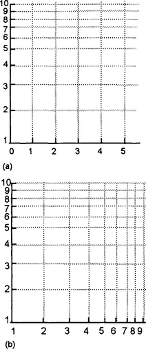
To avoid having to take the logarithms of quantities, it is possible to use special graph paper which effectively takes the logarithms for you. Figure 1.64 shows the form taken by log-linear and log-log graph paper. On a logarithmic scale, the distance between 1 and 10 is the same as between 10 and 100, each of these distances being termed a cycle.
It is believed that the relationship between y and x for the following data is of the form y = a ebx. Show that this is the case and determine, using log-linear graph paper, the values of a and b.
![]()
Taking logarithms to base e gives In y = bx + In a. We thus require log-linear graph paper. The y-axis, which is the In axis, has to range from In 5.53 = 1.7 to In 8.24 = 2.1 and so just one cycle from 1 to 10 is required. Figure 1.65 shows the resulting graph. The graph is straight line and so the relationship is valid. The gradient is
The intercept with the y-axis, i.e. x = 0 ordinate, is at 5.

The relationship between power P (in watts), the e.m.f. E (in volts) and the resistance R (in ohms) is thought to be of the form P = En/R. In a test in which R was kept constant, the following measurements were recorded:
![]()
Determine whether the above relationship is true (or approximately so) and determine the values for n and R.
Taking In of both sides of the equation gives:
So, if the relationship is true, a graph of In P against In E should be a straight line. The values of In P and In E are:
![]()
Figure 1.66 shows the plot. From the graph we obtain an intercept on the y-axis of −2.3 and a gradient of about 2.

We thus have −2.3 = − In R and so:
and R = 9.9, or 10 when rounded up. With n = 2 we thus have:
We can test that this is valid by choosing any two results from the test, e.g. E = 5 V, P = 2.5 W and substituting them into the equation. With E = 5 V the equation gives P = 23/10 = 2.5 V and so the test confirms the equation.
Radioactive materials, e.g. uranium 235, decay and the mass of that isotope decreases with time. The rate of decay of the isotope is proportional to the mass of isotope present:
where λ is a constant called the decay constant. If m0 is the mass at time t = 0 and mass m the mass at time t, then the following relationship can be derived from the above equation:
A graph of In m plotted against t will be a straight line graph of slope −λ and intercept +ln m0.
Problems 1.7
1. Simplify (a) 2 lg x + log x2, (b) In 2x3 − In(4/x2).
2. Write the following in terms of lg a, Ig b and lg c:
3. Solve for x the equations: (a) 3x = 300, (b) 102−3x = 6000, (c)72x+1 = 43−x.
4. The following data indicates how the voltage v across a component in an electrical circuit varies with time t. It is considered that the relationship between V and t might be of the form v = V e−bt. Show that this is so and determine the values of V and b.
![]()
5. A hot object cools with time. The following data shows how the temperature θ of the object varies with time t. The relationship between θ and t is expected to be of the form θ = a e−bx. Show that this is so and determine the values of a and b.
![]()
6. The rate of flow Q of water over a V-shaped notch weir was measured for different heights h of the water above the point of the V and the following data obtained. The relationship between Q and h is thought to be of the form Q = ahb. Show that this is so and determine the values of a and b.
![]()
7. The amplitude A of oscillation of a pendulum decreases with time t and gives the following data. Show that the relationship is of the form A = a ebt and determine the values of a and b.
![]()
8. The tension T and T0 in the two sides of a belt driving a pulley and in contact with the pulley over an angle of q is given by the equation T = T0 eμθ. Determine the values of T0 and μ for the following data:
![]()
9. In an electrical circuit, the current i in mA occurring when an 8.3 μF capacitor is being discharged varies with time t in ms as shown in the following table:
![]()
If I and T are constants, with I being the initial current in mA, show that the above results are connected by the equation i = I et/T and determine I and T.
10. The pressure P at a height h above ground level is given by P = P0 e−h/c, where P0 is the pressure at ground level and c is a constant. When P0 is 1.013 × 10⁵ Pa and the pressure at a height of 1570 m is 9.871 × 10⁴ Pa, determine graphically the value of c.
1.8 Hyperbolic functions

When we want to describe the curve a rope hangs in we use, what is termed, an hyperbolic function. The sine, cosine and tangent are termed circular functions because their definition is associated with a circle. In a similar way, the sinh (pronounced sinch or shine), cosh (pronounced cosh) and tanh (pronounced than or tanch) are hyperbolic functions associated with a hyperbola. Sinh is a contracted form of ‘hyperbolic sine’, cosh of ‘hyperbolic cosine’ and tanh of ‘hyperbolic tangent’. Figure 1.67 shows the comparison of the circular and hyperbolic functions. The hyperbolic functions are defined as:
Also we have sech x = 1/cosh x, cosech x = 1/sinh x and coth x = 1/tanh x.
1.8.1 Graphs of hyperbolic functions
Since cosh x is the average value of ex and e−x we can obtain a graph of cosh x as a function of x by plotting the ex and e−x graphs and taking the average value. Figure 1.68 illustrates this. Note that unlike cos x, cosh x is not a periodic function. At x = 0, cosh x = 1. The curve is symmetrical about the y-axis, i.e. cosh (−x) = cosh x and is termed an even function.

To obtain the graph of sinh x from those of ex and e−x, at a particular value of x we subtract the second from the first and then take half the resulting value. Figure 1.69 illustrates this. Note that unlike sin x, sinh x is not a periodic function. When x = 0, sinh x = 0. The curve is symmetrical about the origin, i.e. sinh(−x) = −sinh x, and is said to be an odd function.

Figure 1.70 shows the graph of tanh x, obtained by taking values of ex and e−x and calculating values of tanh x for particular values of x. Unlike tan x, tanh x is not periodic. When x = 0, tanh x = 0. All the values of tanh x lie between −1 and +1. As x tends to infinity, tanh x tends to 1. As x tends to minus infinity, tanh x tends to −1. The curve is symmetrical about the origin, i.e. tanh(−x) = −tanh x, and is said to be an odd function.

Hyperbolic functions and suspended cables
Often it is necessary for engineers to analyse frameworks in order to test for their integrity, i.e. safety and ability to function as designed under a range of conditions. The design engineer needs to formulate a mathematical ‘model’ which will accurately represent the real system when built. Such problems often involve hyperbolic functions as the following example shows.
Consider a uniform cable which is suspended from two fixing points A and B and which hangs under its own weight (Figure 1.71). Point A is higher than point B and the cable has a uniform weight μ per unit length.

By drawing free-body diagrams for the forces involved on an element of the cable and considering its equilibrium we can arrive at a differential equation (see chapter 4 for a discussion of such equations), which when solved leads to the equation for the gradient a distance x from P:
T0 is the horizontal component of the tension in the cable at P. This equation can then give (by integration, see chapter 4) the height y above P of the cable at distance x as:
where k is a constant. Since x = 0 when y = 0, we can put these values in the equation and obtain k = −T0/μ. Thus:
This is the equation of the curve of the cable, known as a catenary. For a full analysis of the system, see the companion book in this series: Mechanical Engineering Systems by R. Gentle, P. Edwards and W. Bolton
Problems 1.8
1. Determine, using a calculator, the values of (a) sinh 2, (b) cosh 5, (c) tanh 2, (d) sinh(−2), (e) cosech 1.4, (0 sech 0.8.
2. A flexible cable suspended between two horizontal points hangs in the form of a catenary (Figure 1.72), the equation of the curve being given by y = c[cosh(x/c) − 1], where y is the sag of the cable, x the horizontal distance from the midpoint to one end of the cable and c is a constant. Determine the sag of a cable when c = 20 and 2x = 16 m.

Figure 1.72 Problem 2
3. The speed v of a surface wave on a liquid is given by:

where g is the acceleration due to gravity, λ the wavelength of the waves, γ the surface tension, ρ the density and h the depth of the water. What will the speed approximately be for (a) shallow water waves when h/k tends to zero, (b) deep water waves when h/k tends to infinity?