
Mathematical models
3.1 Modelling
• Tall buildings are deflected by strong winds, can we devise a model which can be used to predict the amount of deflection of a building for particular wind strengths?
• Cars have suspension systems, can we devise a model which can be used to predict how a car will react when driven over a hump in the road?
• When a voltage is connected to a d.c. electrical motor, can we devise a model which will predict how the torque developed by the motor will depend on the voltage?
• Can we devise a model to enable the optimum shaft to be designed for a power transmission system connecting a motor to a load?
• Can we design a model to enable an appropriate transducer to be selected as part of the monitoring/activation circuit for the safe release of an air bag in a motor vehicle under crash conditions?
• Can we design models which will enable failure to be predicted in static and dynamic systems?
• Can we design models to enable automated, robotic controlled systems to be designed?
With reference to Figure 3.1 and point 5, together with any reconsideration of the problem, quite often this involves the formulation of a computer model. The aim is to use the computer model to ‘speed’ up the analysis of the mathematical model in order to compare the results with collected data from the real world. Such software models therefore have to be benchmarked against the mathematical model and real world data to be validated prior to being used.

Such questions as those above are encountered by design and manufacturing system engineers daily. Quite often it is the accuracy of a mathematical model that will determine the success or otherwise of a new design. Such models also greatly help to reduce the design-test-evaluation-manufacture process lead time.
3.1.1 How do we devise models?
The tactics adopted to devise models involve a number of stages which can be summarised by the block diagram of Figure 3.1. The first stage involves identifying what the real problem is and then identifying what factors are important and what assumptions can be made. These assumptions are used in order to simplify the model and enable an initial model to be formulated which we can check as being a reasonable approximation. Only when we are confident with the model do we build in further considerations to make the models even more accurate! For example, when modelling mechanical systems, we often initially ignore friction and the consequential heat generation; however, as the model is refined we have to consider such effects and adjust the initial ‘ball park’ model in order for its application to the real world to be valid. This stage will generally involve collecting data. The next stage is then to formulate a model. An essential part of this is to translate verbal statements into mathematical relationships. When solutions are then produced from the model, they need to be compared with the real world and, if necessary the entire cycle repeated.
Example of formulating a model
As an illustration, consider how we might approach the problem we started this section with:
Tall buildings are deflected by strong winds, can we devise a model which can be used to predict the amount of deflection of a building for particular wind strengths?
The simplest form we might consider is that of a tall building which is subject to wind pressure over its entire height, the building being anchored at the ground but free to deflect at its top (Figure 3.2). If we assume that the wind pressure gives a uniform loading over the entire height of the building and does not fluctuate, then we might consider the situation is rather like the deflection of the free end of a cantilever when subject to a uniformly distributed load (Figure 3.3). For such a beam the deflection y is given by:
where L is the length of the beam, w the load per unit length, E the modulus of elasticity and I the second moment of area. The modulus of elasticity if a measure of the stiffness of the material and the second moment of area for a rectangular section is bd3/12, with b being the breadth and d the depth. This would suggest that a stiff structure would deflect less and also one with a large cross-section would deflect less. Hence we might propose a model of the form:
with p being the wind pressure and related to the wind velocity, H the height of the building, b its breadth and d its depth. Thus, a short, squat building will be less deflected than a tall slender one of the same building materials.


3.1.2 Lumped element modelling
Often in engineering we can devise a model for a system by considering it to be composed of a number of basic elements. We consider the characteristics of the behaviour of the system and ‘lump’ all the similar behaviour characteristics together and represent them by a simple element. For some elements, the relationship between their input and output is a simple proportionality, in other cases it involves a rate of change with time or even the rate of change with time of a rate of change with time.
Mechanical systems
Mechanical systems can be considered to be made up of three basic elements which represent the stiffness, damping and inertia of the system:
The ‘springiness’ or ‘stiffness’ of a system can be represented by a spring (Figure 3.4(a)). The force F is proportional to the extension x of the spring:
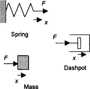
The ‘damping’ of a mechanical system can be represented by a dashpot. This is a piston moving in a viscous medium in a cylinder (Figure 3.4(b)). The damping force F is proportional to the velocity v of the damping element:
where c is a constant. Since the velocity is equal to the rate of change of displacement x:
The ‘inertia’ of a system, i.e. how much it resists being accelerated can be represented by mass m. Since the force F acting on a mass is related to its acceleration a by F = ma and acceleration is the rate of change of velocity, with velocity being the rate of change of displacement x:
To develop the equations relating inputs and outputs we use Newton’s laws of motion.
Develop a lumped-model for a car suspension system which can be used to predict how a car will react when driven over a hump in the road (the second problem listed earlier in this chapter).
Such a system can have its suspension represented by a spring, the shock absorbers by a damper and the mass of the car and its passengers by a mass. The model thus looks like Figure 3.5(a). We can then devise an equation showing how the output of the system, namely the displacement of the passengers with time depends on the input of the displacement of a car wheel as it rides over the road surface.
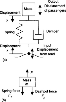
This is done by considering a free-body diagram, this being a diagram of the mass showing just the external forces acting on it (Figure 3.5(b)). We can then relate the net force acting on the mass to its acceleration by the use of Newton’s law, hence obtaining an equation which relates the input to the output.
The relative extension of the spring is the difference between the displacement x of the mass and the input displacement y. Thus, the force due to the spring Fs is k(x − y). The dashpot force Fd is c(dx/df − dy/dt). Hence, applying Newton’s law:
and so we can write:
Rotational systems
For rotational systems, e.g. the drive shaft of a motor, the basic building blocks are a torsion spring, a rotary damper and the moment of inertia (Figure 3.6).

Figure 3.6 Rotational system elements: (a) torsional spring, (b) rotational dashpot, (c) moment of inertia
The ‘springiness’ or ‘stiffness’ of a rotational spring is represented by a torsional spring. The torque T is proportional to the angle θ rotated:
where k is a constant.
The damping inherent in rotational motion is represented by a rotational dashpot. The resistive torque T is proportional to the angular velocity ω and thus, since ω is the rate of change of angle θ with time:
where c is a constant.
The inertia of a rotational system is represented by the moment of inertia I of a mass. The torque T needed to produce an acceleration a is given by T = Iα and thus, since α is the rate of change of angular velocity ω with time and angular velocity is the rate of change of angle θ with time:
Represent as a lumped-model the system shown in Figure 3.7(a) of the rotation of a disk as a result of twisting a shaft.
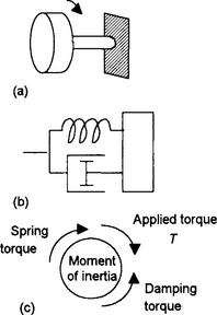
Figure 3.7(b) shows the lumped-model and Figure 3.7(c) the free-body diagram for the system.
The torques acting on the disk are the applied torque, the spring torque and the damping torque. The torque due to the spring is kθ and the damping torque is c(dθ/dt). Hence, since the net torque acting on the mass is:
we have:
Electrical systems
The basic elements of electrical systems are the resistor, inductor and capacitor (Figure 3.8).

The resistor represents the electrical resistance of the system. The potential difference v across a resistor is proportional to the current i through it:
The inductor represents the electrical inductance of the system. For an inductor, the potential difference v across it depends on the rate of change of current i through it and we can write:
The capacitor represents the electrical capacitance of the system. For a capacitor, the charge q on the capacitor plates is related to the voltage v across the capacitor by q = Cv, where C is the capacitance. Since current i is the rate of movement of charge:
To develop the models for systems which we describe by electrical circuits involving resistance, inductance and capacitance we use Kirchhoff’s laws.
Develop a lumped-system model for a d.c. motor relating the current through the armature to the applied voltage.
The motor consists basically of the armature coil, this being free to rotate, which is located in the magnetic field provided by either a permanent magnet or a current through field coils. When a current flows through the armature coil, forces acting on as a result of the current carrying conductors being in a magnetic field. As a result, the armature coil rotates. Since the armature is a coil rotating in a magnetic field, a voltage is induced in it in such a direction as to oppose the change producing it, i.e. there is a back e.m.f. Thus the electrical circuit we can use to describe the motor has two sources of e.m.f., that applied to produce the armature current and the back e.m.f. If we consider a motor where there is either a permanent magnet or separately excited field coils, then the lumped electrical circuit model is as shown in Figure 3.9. We can consider there are just two elements, an inductor and a resistor, to represent the armature coil. The equation is thus:
This can be considered to be the first stage in addressing the problem posed earlier in the chapter: When a voltage is connected to a d.c. electrical motor, can we devise a model which will predict how the torque developed by the motor will depend on the voltage? The torque generated will be proportional to the current through the armature.

Thermal systems
Thermal systems have two basic building blocks with thermal systems, resistance and capacitance.
The thermal resistance R is the resistance offered to the rate of flow of heat q and is defined by:
where T1 − T2 is the temperature difference through which the heat flows.
For heat conduction through a solid we have the rate of flow of heat proportional to the cross-sectional area A and the temperature gradient. Thus, for two points at temperatures T1 and T2 and a distance L apart, we can write:
with k being the thermal conductivity. With this mode of heat transfer, the thermal resistance R is L/Ak.
For heat transfer by convection between two points, Newton’s law of cooling gives:
where (T2 − T1) is the temperature difference, h the coefficient of heat transfer and A the surface area across which the temperature difference is. The thermal resistance with this mode of heat transfer is thus 1/Ah.
The thermal capacitance is a measure of the store of internal energy in a system. If the rate of flow of heat into a system is q1 and the rate of flow out q2 then the rate of change of internal energy of the system is q1− q2. An increase in internal energy can result in a change in temperature:
where m is the mass and c the specific heat capacity. Thus the rate of change of internal energy is equal to mc times the rate of change of temperature. Hence:
This equation can be written as:
where the capacitance C = mc.
Develop a lumped-model for the simple thermal system of a thermometer at temperature T being used to measure the temperature of a liquid when it suddenly changes to the higher temperature of TL (Figure 3.10).
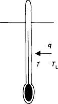
When the temperature changes there is heat flow q from the liquid to the thermometer. If R is the thermal resistance to heat flow from the liquid to the thermometer then q = (TL − T)/R. Since there is only a net flow of heat from the liquid to the thermometer, if the thermal capacitance of the thermometer is C, then q = C dT/dt.
Hydraulic systems
For a fluid system the three building blocks are resistance, capacitance and inertance. Hydraulic fluid systems are assumed to involve an incompressible liquid; pneumatic systems, however, involve compressible gases and consequently there will be density changes when the pressure changes. Here we will just consider the simpler case of hydraulic systems. Figure 3.11 shows the basic form of building blocks for hydraulic systems.
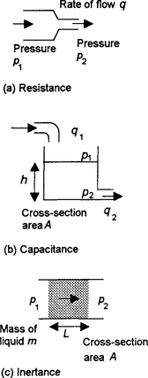
Hydraulic resistance R is the resistance to flow which occurs when a liquid flows from one diameter pipe to another (Figure 3.11(a)) and is defined as being given by the hydraulic equivalent of Ohm’s law:
Hydraulic capacitance C is the term used to describe energy storage where the hydraulic liquid is stored in the form of potential energy (Figure 3.11(b)). The rate of change of volume V of liquid stored is equal to the difference between the volumetric rate at which liquid enters the container q1 and the rate at which it leaves q2, i.e.
But V = Ah and so:
The pressure difference between the input and output is:
Hence, substituting for h gives:
The hydraulic capacitance C is defined as:
Hydraulic inertance is the equivalent of inductance in electrical systems. To accelerate a fluid a net force is required and this is provided by the pressure difference (Figure 3.11(c)). Thus:
where a is the acceleration and so the rate of change of velocity v. The mass of fluid being accelerated is m = ALρ and the rate of flow q = Av and so:

where the inertance I is given by I = Lρ/A.
Develop a model for the hydraulic system (Figure 3.12) where there is a liquid entering a container at one rate q1 and leaving through a valve at another rate q2.

We can neglect the inertance since flow rates can be assumed to change only very slowly. For the capacitance term we have:
For the resistance term for the valve we have p1 − p2 = Rq1. Thus, substituting for q2, and recognising that the pressure difference is hρg, gives:
Problems 3.1
1. Propose a mathematical model for the oscillations of a suspension bridge when subject to wind gusts.
2. Propose a mathematical model for a machine mounted on firm ground when the machine is subject to forces when considered in terms of lumped-parameters.
3. Derive an equation for a mathematical model relating the input and output for each of the lumped systems shown in Figure 3.13.

Figure 3.13 Problem 3
3.2 Relating models and data
In testing mathematical models against real data, we often have the situation of having to check whether data fits an equation. If the relationship is linear, i.e. of the form y = mx + c, then it is comparatively easy to see whether the data fits the straight line and to ascertain the gradient m and intercept c. However, if the relationship is non-linear this is not so easy. A technique which can be used is to turn the non-linear equation into a linear one by changing the variables. Thus, if we have a relationship of the form y = ax2 + b, instead of plotting y against x to give a non-linear graph we can plot y against x2 to give a linear graph with gradient a and intercept b. If we have a relationship of the form y = a/x we can plot a graph of y against 1/x to give a linear graph with a gradient of a.
The following data was obtained from measurements of the load lifted by a machine and the effort expended. Determine if the relationship between the effort E and the load W is linear and if so the relationship.
![]()
Within the limits of experimental error the results appear to indicate a straight-line relationship (Figure 3.14). The gradient is 41/200 or about 0.21. The intercept with the E axis is at 10. Thus the relationship is E = 0.21 W + 10.

It is believed that the relationship between y and x for the following data is of the form y = ax2 + b. Determine the values of a and b.
![]()
Figure 3.15 shows the graph of y against x2. The graph has a gradient of AB/BC = 12.5/25 = 0.5 and an intercept with the y-axis of 2. Thus the relationship is y = 0.5x2 + 2.

Problems 3.2
1. Determine, assuming linear, the relationships between the following variables:
(a) The load L lifted by a machine for the effort E applied.
![]()
(b) The resistance R of a wire for different lengths L of that wire.
![]()
2. Determine what form the variables in the following equations should take when plotted in order to give straight-line graphs and what the values of the gradient and intercept will have.
(a) The period of oscillation T of a pendulum is related to the length L of the pendulum by the equation:
where g is a constant.
(b) The distance s travelled by a uniformly accelerating object after a time t is given by the equation:
where u and a are constants.
(c) The e.m.f. e generated by a thermocouple at a temperature θ is given by the equation;
where a and b are constants.
(d) The resistance R of a resistor at a temperature h is given by the equation:
where R0 and α are constants.
(f) The pressure p of a gas and its volume V are related by the equation:
(g) The deflection y of the free end of a cantilever due to it own weight of w per unit length is related to its length L by the equation:
where w, E and I are constants.
3. The resistance R of a lamp is measured at a number of voltages V and the following data obtained. Show that the law relating the resistance to the voltage is of the form R = (a/V) + b and determine the values of a and b.
![]()
4. The resistance R of wires of a particular material are measured for a range of wire diameters d and the following results obtained. Show that the relationship is of the form R = (a/d2) + b and determine the values of a and b.
![]()
5. The volume V of a gas is measured at a number of pressures p and the following results obtained. Show that the relationship is of the form V = apb and determine the values of a and b.
![]()
6. When a gas is compressed adiabatically the pressure p and temperature T are measured and the following results obtained. Show that the relationship is of the form T = aρb and determine the values of a and b.
![]()
7. The cost C per hour of operating a machine depends on the number of items n produced per hour. The following data has been obtained and is anticipated to follow a relationship of the form C = an3 + b. Show that this is the case and determine the values of a and b.
![]()
8. The following are suggested braking distances s for cars travelling at different speeds v. The relationship between s and v is thought to be of the form s = av2 + bv. Show that this is so and determine the values of a and b.
![]()
Hint: consider s/v as one of the variables.
9. The luminosity I of a lamp depends on the voltage V applied to it. The relationship between I and V is thought to be of the form I = aVb. Use the following results to show that this is the case and determine the values of a and b.
![]()
10. From a lab test, it is believed that the law relating the voltage v across an inductor and the time t is given by the relationship v = A et/B, where A and B are constant and e is the exponential function. From the lab test the results observed were:
![]()
Show that the law relating the voltage to time is, in fact, true. Then determine the values of the constants A and B.