

Example 7.6
Starting from pyrite, plot the equilibrium curve for various pressures (0.8 atm, 1 atm, 1.2 atm) and initial concentrations of SO2 to the converter (6%, 8%, 10%).
Solution
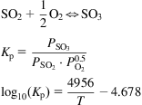
Consider the reaction stoichiometry and the equilibrium constant for the oxidation of SO2:
Assume 1 kmol of dry air. The mass balances for the pyrite roasting and the sulfur dioxide conversion are as follows (Table 7E6.1):
Table 7E6.1
Balances to Pyrite Roasting and Equilibrium Stages
| FeS2+(11/4)O2→0.5Fe2O3+2SO2 | SO2→SO3 | |||
| Initial | Final | Initial | Equilibrium | |
| SO2 | – | 2a | 2a | 2·a·(1−X) |
| N2 | 0.79 | 0.79 | 0.79 | 0.79 |
| O2 | 0.21 | 0.21−2.75a | 0.21−2.75a | 0.21−2.75a −a·X |
| SO3 | – | 2·a·X | ||

The fraction of SO2 in the gas that enters the converter is given by:
In the equilibrium, the total number of moles is given by the equation below:
Therefore, the partial pressures for the species involved are the following:

The equilibrium constant is given by this equation:

Fig. 7E6.1 shows the effect of feed composition, operating pressure, and temperature on the conversion.

Example 7.7
Multibed reactor design: A production facility operates a four bed reactor. The feedstock enters the reactor at 400°C with an SO2 content of 10% from burning sulfur. The total pressure is 1 atm. The feed temperatures before the second, third, and fourth beds are 450°C, 450°C, and 430°C, respectively. Each catalytic bed reaches 97% of the equilibrium conversion and operates adiabatically. Determine the gas composition after each bed.
Solution
Using the results presented in Example 7.5, with a=0.1, we compute the equilibrium line. As before, from sulfur, and considering 1 kmol of dry air, we have the mass balances as seen in Table 7E7.1.
Table 7E7.1
Balances to Sulfur Burning and Equilibrium Stages
| S→SO2 | SO2→SO3 | |||
| Initial | Final | Initial | Equilibrium | |
| SO2 | – | a | a | a·(1−X) |
| N2 | 0.79 | 0.79 | 0.79 | 0.79 |
| O2 | 0.21 | 0.21−a | 0.21−a | 0.21−a−0.5·a·X |
| SO3 | – | a·X | ||

The moles in the equilibrium are as follows:
The equilibrium constant can be computed as below (and plotted in Fig. 7E7.1):


For the first bed, we perform an energy balance:

Assuming constant heat capacity for the mixture and the fact that the moles of gas are almost constant in the bed, the balance becomes linear:

This straight line reaches the equilibrium line. For the sake of argument, we fit the equilibrium curve to a polynomial as a function of temperature in order to solve the conversion at each bed. X is the conversion, and T is the temperature in K:
By solving the energy balance and the equilibrium line simultaneously, we have X=0.7 and T=881K; see Fig. 7E7.2. However, the conversion is only 97% of that: 0.686.

For the second bed, the gas is cooled with no progress in the conversion; see the horizontal line in Fig. 7E7.3. The energy balance uses the flow rate exiting the first bed as a starting point and assumes that there is not a large change in the flow across the bed. Note that the equilibrium is computed with respect to total conversion and therefore X is the global conversion, not the one reached at each bed. Thus, the energy balance becomes (Fig. 7E7.3):


By solving the equilibrium and the energy balance we have X=0.91 at T=787K. Again, only 97% of the equilibrium is reached; thus, X=0.89. For the third bed, the procedure is repeated. The energy balance is as follows:

The conversion becomes 0.97 at 739K. Thus 0.94 is the actual conversion (Fig. 7E7.4).

For the last bed we have the following:

The computed conversion is 0.98 at 722K. The actual one is 0.95; see Fig. 7E7.5.

The summary of the mass balances for each of the beds is presented below. Note that the total molar flow is the one used as nT,ini for each bed (Table 7E7.2).

7.3.3.3.2 Oxidation kinetics
In the previous section, only the equilibrium is evaluated to design the reactor. However, the bed depth depends on the kinetics, which is a function of the catalysts—platinum, iron oxide, and V2O5 (Fogler, 1997).
The mechanism of the reaction is suggested to be the following:
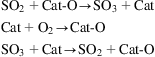
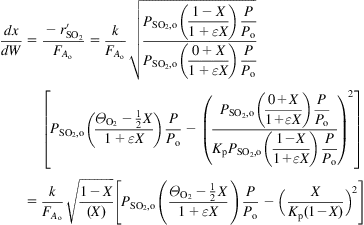
The kinetics of the reaction were established by Eklund (1956):
(7.4)
where k is a function of the catalyst and the geometry, and Pi is the partial pressure of each species. For the example, based on the data from Eklund’s paper, the catalyst is V2O5 supported on volcanic rock with a volumetric density of 33.8 lb/ft3. In the following example, we determine the depth of a catalytic bed in a converter for SO3 production.
Example 7.8
The first bed of a converter is fed with a flow rate of 467.1292 mol/s at 2 atm and 750K. Out of that, 51.42 mol/s is SO2. The aim is to reach 50% conversion at the end of the bed. The diameter of the converter is 6.650 m, and the catalyst properties, porosity, particle diameter, and apparent density are given below. Determine the depth of the catalytic bed.
Solution
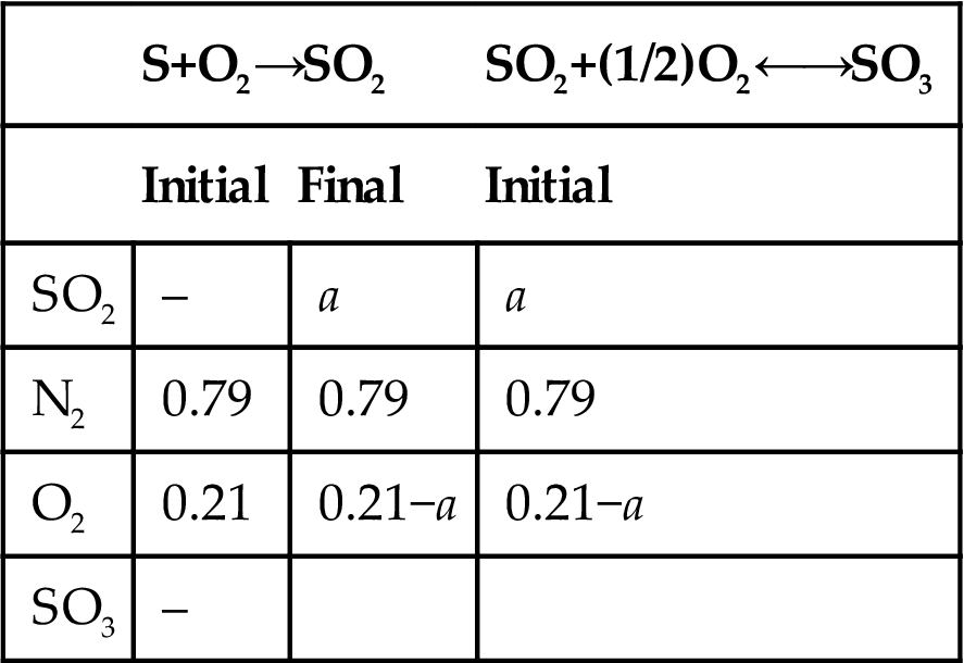
We assume a plug flow reactor where the sulfur dioxide comes from sulfur burning. With the information provided, and a=0.11, the mass balance for the sulfur burner and the first bed is as shown in Table 7E8.1.
Table 7E8.1
Mass Balance for SO3 Production From Sulfur
| S+O2→SO2 | SO2+(1/2)O2←→SO3 | ||
| Initial | Final | Initial | |
| SO2 | – | a | a |
| N2 | 0.79 | 0.79 | 0.79 |
| O2 | 0.21 | 0.21−a | 0.21−a |
| SO3 | – | ||
Kinetics of the reactor:
If the conversion is below 5%, the reaction rate does not depend on the conversion, and is therefore given as:
The reaction rate is given by:
The equilibrium constant is given as:
Kp [=] Pa−0.5, T [=] K
For the rate constant (based on Eklund’s (1956) results) we have:
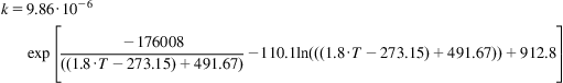
k is in mol of SO2/kg cat S·Pa, while T is in K.
The stoichiometrics of the reaction are as follows:

Assuming ideal gases:

Dividing both:
The concentration of the species i is as follows:

Dividing both:

Thus, the partial pressure of component i is the following:

Therefore, the kinetics of the reaction become:

FAo=51.42 mol/s
The energy balance is as follows:

Assuming adiabatic operation of the bed:

Thus the heat of reaction is computed as:

where cp is in J/mol K, and temperature (T) is in K (Sinnot, 1999):

The pressure drop along the tube is given by the Ergun equation:
G is the superficial mass velocity (kg/m2 s), ϕ is the porosity of the bed, Dp is the particle diameter (m), μ is the viscosity of the gas (Pa·s), and ρ is the gas density (kg/m3) that can be found in Fogler (1997):

To solve the problem we use MATLAB. For further notes on the use of MATLAB for solving chemical reactors we refer the reader to Martín (2014).
M file: ReactorSO2
[a,b]=ode15s(‘ReacSI’,[0 5000],[0,750,202650]);
plot(a,b(:,1))
xlabel(‘W (kg)’)
ylabel(‘X’)
figure
plot(a,b(:,2))
xlabel(‘W (kg)’)
ylabel(‘T (K)’)
figure
plot(a,b(:,3))
xlabel(‘W (kg)’)
ylabel(‘P (Pa)’)
M file: Reac
function Reactor=ReacSI(w,x)
X=x(1);
T=x(2);
Presion=x(3);
k=9.8692e−3*exp(−176008/(1.8*(T−273.15)+491.67) −110.1*log((1.8*(T-273.15)+491.67))+912.8);
Kp=0.0031415*exp(42311/(1.987*(1.8*(T−273.15)+491.67) )−11.24);
Pto=202650;
ySO2o=0.11;
yO2o=0.1;
yN2o=0.79;
PhiO2=yO2o/ySO2o;
PSO2o=Pto*ySO2o;
Fto=467.1292;
Fao=Fto*ySO2o;
epsilon=-0.055;
G=0.433;
ph=0.45;
rhoo=0.866;
Dp=0.00457;
visc=3.72e-5;
Ac=3.14*(6.650/2)^2;
rhob=542;
To=750;
sumCp=272.77−0.0303*T+0.000158*T^2−8.016e−8*T^3;
dCp=−21.535+0.0789*T−7.112*10^(−5)*T^2+2.447e−8*T^3;
deltaHr=−98480−21.535*(T−298)+0.0395*(T^2−298^2)−2.371*10^(−5)*(T^3−298^3)+6.117*10^(−9)*(T^4−298^4);
if X<0.05;
ra=−k*((1−0.05)/0.05)^(0.5)*(PSO2o*((PhiO2−0.5*X)/(1+epsilon*0.05))*(Presion/Pto)−(0.05/(Kp*(1−0.05)))^2);
else
ra=−k*((1-X)/X)^(0.5)*(PSO2o*((PhiO2−0.5*X)/(1+epsilon*X))*(Presion/Pto)−(X/(Kp*(1−X)))^2);
end
Reactor(1,1)=−ra/Fao;
Reactor(2,1)=((−ra)*(−deltaHr))/(Fao*(sumCp+X*dCp));
Reactor(3,1)=−G*(1−ph)*(1+epsilon*X)*Pto*T*(150*(1−ph)*visc/Dp+1.75*G)/(rhob*Ac*rhoo*Dp*ph^3*To*Presion);
The solution is summarized in the two figures below for the conversion and the temperature profiles. We need 1600 kg of catalyst. We see that the temperature increases 120K since it operates adiabatically (Fig. 7E8.1).

Based on the geometry of the converter and the density, we need:

7.3.3.3.3 SO3 absorption
The SO3 produced is sent to absorption columns where it is put into contact with water. Typically, the water remains in a solution of sulfuric acid. It is a chemical absorption:
The process is highly exothermic, and the formation enthalpy of sulfuric acid is as follows:
Apart from the formation itself, if the sulfuric acid is diluted, solution enthalpies must be considered too. In this section we design one such a column.
Example 7.9
Compute the length of an absorption tower for the production of H2SO4 so that we absorb 95% of the incoming SO3. Assume isothermal operation (Fig. 7E9.1).

Solution
The kinetics are as follows:
However, the reaction rate is limited by diffusion:
where r is the ratio between the film thickness for absorption and that for chemical reaction. According to Krevelen and Hoftyzer (Goodhead and Abowei, 2014), r is defined as:
where KL is the mass transfer coefficient, and DL is the SO3 diffusivity. Therefore, the reaction rate becomes:
Based on basic reaction kinetics of a bimolecular reaction, the converted mass is computed as ![]() . Thus, the equation becomes:
. Thus, the equation becomes:
Assuming that the tower behaves as a plug flow reactor, the design equation becomes:
Rearranging the terms:


Table 7E9.1 gives information on the parameters needed for the tower design.
Table 7E9.1
| 15 | mol/m3 | |
| k2 | 0.3 | 1/s |
| 4 | mol/s | |
| DR | 0.1 | m |
| m | 1 | |
| DL | 17 | m2/s |
| Vo | 2.3×10⁻⁴ | m3/s |

It is assumed that the tower operates isothermally. Thus, the energy to be removed is computed as:
Solving the problem, we have L=34.7 m.
Apart from the kinetics, the flow through a tower has a pressure drop. The pressure drop across the absorption tower is given by the Ergun equation, and depends on the type of packing. An empirical correlation was developed by Cameron and Chang (2010):
(7.5)
The pressure drop given by Eq. (7.5) must be corrected to include that of the loading region so that:
(7.6)
where C2, C3, and C4 are adjustable parameters that can be seen in Table 7.4. VL is the irrigation rate (ft/s) based on an empty tower. Fs is the ratio between the gas velocity across an empty tower and the density as V/ρ0.5, and ε is the porosity of the tower, typically around 0.75.
Table 7.4
Coefficients for Pressure Drop Estimation (Cameron and Chang, 2010)
| Packing Type | Size (in) | C2 | C3 | C4 |
| Standard saddle | 1 | 0.69 | 22.33 | 1.6 |
| Standard saddle | 1.5 | 0.38 | 22.33 | 1.6 |
| Standard saddle | 2 | 0.21 | 22.33 | 1.6 |
| Standard saddle | 3 | 0.15 | 22.33 | 1.6 |

The diameter is computed (as in typical absorption towers) using the loading line for determining the K parameter, and the following set of equations (Sinnot, 1999):
(7.7)
 (7.7)
(7.7)
7.3.3.3.4 Mixing tanks: heat of solution
When mixing acids or acid solutions there is a certain energy involved. In Fig. 7.11 the integral heat of solution for sulfuric acid is presented at 25°C. The mixture is exothermic and can result in the evaporation of water. Therefore, apart from the health and safety issues related to acid solution mixing, the concentration of the resulting mixture is to be carefully computed to account for that (Houghen et al., 1959). Example 7.10 presents such a case. We compute the energy involved in the mixing using enthalpy concentration diagrams.

Example 7.10
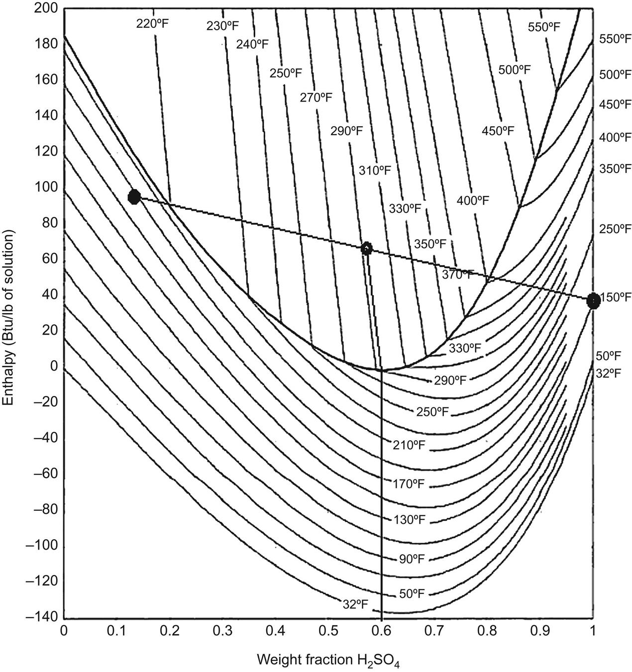
Mixtures of water and sulfuric acid solutions. A flow rate of 1 kg/s of H2SO4 at 70°C is mixed with a solution of 1 kg/s of a solution of 15% H2SO4 at 85°C in a tank at 1 atm. Determine the composition of the final mixture.
Solution
We can determine the final composition using the integral heat of dilution, but it is easier to use an enthalpy diagram (see below). We locate the points for both solutions in the diagram. The lever rule can be used as a rough estimate to identify whether there will be water evaporation or not. We see that for a 1:1 mixture the product will be above the boiling point curve. Therefore, the energy generated is enough to boil the water.
Performing a mass balance we compute the point if no water is evaporated:
Using Fig. 7E10.1, the composition of the final liquid mixture is determined by projecting the point into the boiling point curve (as presented in the figure). Thus, the composition of the liquid mixture is 60% sulfuric acid, and the rest of the water has evaporated.
Now we compute the composition by performing mass and energy balances:
If the mixture reaches the boiling point and the water evaporates, it is concentrated. For a mixture of 57.5%, its enthalpy becomes:
The energy balance states that the flow enthalpy of the feed streams is as follows:
Then, the mixture evaporates water. Therefore, the mass and energy balances must be rewritten to account for water evaporation:

To solve the system, we assume y, compute xm, and see if the energy balance holds. Alternatively, since we already have an estimate for the concentration of the mixture from the diagram, we can use that as xm and compute the water that evaporates:
The boiling point is 290°F (ie, 143°C).
Thus the enthalpy of the overheated steam is as follows:
The small difference is due to reading the enthalpy values in the figure. Thus approximately 0.1 is the fraction evaporated.
7.4 Problems
P7.1. A mixture of SO2, O2, and N2 from sulfur burning with dry air is fed to a converter. The mixture contains 8% per volume of SO2. The gas is fed to the converter at 415°C and 1 atm. The converter oxidizes SO2 to SO3 using two beds with intercooling. Assume that the equilibrium conversion is reached at each of the beds (which operate adiabatically). Select between both equilibrium curves below (Fig. P7.1A and B). Determine the composition of the gases exiting each bed and the cooling temperature after the second. Compute the temperature at which the gases from the first bed must be cooled down to so that the final conversion is 95%.

P7.2. A mixture of SO2, O2, and N2 from sulfur burning with dry air is fed to a converter. The converter oxidizes SO2 to SO3 using two beds with intercooling. The gas is fed to the converter at 415°C and 1 atm. The conversion obtained is 95% and the gases exit at 767K. The gases are fed to the second bed at 450°C. Assume that the equilibrium conversion is achieved at each bed and that both operate adiabatically. Plot the equilibrium curve under the operating conditions, and compute the conversion reached after the first bed and the composition of the gases entering and exiting the converter.

P7.3. A mixture of SO2, O2, and N2 from sulfur burning using dry air is fed to a converter. The mixture contains 10% per volume of SO2. The gas is fed to the converter at 415°C and 1 atm. The converter oxidizes SO2 to SO3 using two beds with intercooling. Assume that the equilibrium conversion is reached at each one of the beds (which operate adiabatically). After the first bed, the stream is sent to an absorption tower where all the SO3 is removed. The gases are recycled to the reactor and fed to the second bed at 450°C. Determine the equilibrium curve for each bed and the conversion after the first bed as well as the global conversion of the converter.


P7.4. Sulfur dioxide for the production of sulfuric acid is produced from pyrite roasting. The furnace is fed with pyrite (FeS2) that contains moisture and inert slag. The facilities manager believes that the composition in the contract is not correct based on the products obtained. Air is fed at 25°C and 700 mmHg with a relative humidity of 40%. The gas product has a dew point of 12.5°C and the furnace is operated with twice the stoichiometric oxygen. The slag collected after 10 min contains 0.36 t of FeS, 36 t of Fe2O3, and 6.6 t of inert slag. Determine the composition of the mineral that was sold to the plant and the heat losses, assuming cp,slag=0.16 kcal/kg K and the pyrite is fed to the furnace at 25°C.
P7.5. The gases from pyrite burning are fed to a Glover Tower where a fraction of the SO2 is transformed into H2SO4. Together with the gas, a stream consisting of 592 kg (77% H2SO4, 22% H2O, and 1% N2O3) comes from a Gay-Lussac Tower, and another one from lead chambers (178 kg of H2SO4, 64%); we feed 1.32 kg of HNO3 as catalyst makeup. From the tower we obtain 770 kg of acid (78%); see Fig. P7.5. Determine the conversion of SO2 and the composition of the product gas.
P7.6. Determine the conversion reached in a 25 m tall tower for the absorption of SO3 to produce H2SO4. Assume that the kinetic rate is given by the following equation:
P7.7. The feed to the chambers (at 91°C) is given in Table P7.7. Water is fed at 25°C. The unconverted gases have a dew point of 2°C at 1 atm. These gases are fed to the Gay-Lussac Tower at 40°C. The liquid product, 178 kg of sulfuric acid (64% by weight), exits the chambers at 91°C. Compute the conversion of SO2 in the lead chambers, the water added, and an energy balance to the lead chambers. See Fig. P7.7 for the process scheme.
P7.8. A stream of 467.1292 mol/s at 2 atm and 750K is fed to a catalytic multibed converter. The gas comes from burning sulfur, and 51.42 mol/s of the stream is SO2. Determine the equilibrium conversion and the final temperature after the first catalytic bed. The converter has a diameter of 6.650 m; the catalyst features are given below:
P7.9. Compute the amount of sulfuric acid 98% required to absorb 99.9% of the SO3 in the gases from the third catalytic bed (see Table P7.9), and the acid temperature. The product has a composition of 99%, the gases are at 200°C, and the acid is fed at 90°C. The unabsorbed gases exit at 90°C and we remove 6500 kcal/s using cooling.
P7.10. Evaluate a sulfuric acid production facility that uses the contact method with one absorber. Humid air at 25°C and relative humidity of 0.55 is dried using sulfuric acid 99%, the product. The acid gets diluted to 98% and is used to absorb SO3 produced at the converter. Assume that the molar ratio of dry air to sulfur is 10:1. Sulfur is burned with the dry air to produce SO2. The gas mixture is sent to the converter, which achieves 98% conversion to SO3. This stream is sent to the absorber. In the absorber, water, sulfuric acid 98%, and the gas are put into contact so that sulfuric acid 99% is produced. Compute the amount of sulfuric acid produced (99%), the flowrate of H2SO4 98%, the flow rate of water fed to the absorption tower, and the fraction of sulfuric acid used to dry the initial air. Determine the temperature of operation at the converter assuming isothermal operation at 1 atm.
P7.11. Evaluate a sulfuric acid production facility that uses the contact method with one absorber. Humid air at 25°C and relative humidity of 0.55 is dried using sulfuric acid 99%, the product. The acid gets diluted to 98% and is used to absorb SO3 produced at the converter. Assume that the molar ratio of dry air to sulfur is 10:1. Sulfur is burned with the dry air producing SO2. The gas mixture is sent to the converter, which operates isothermally at 1.5 atm and 700K. This stream is sent to the absorber. In the absorber, water, sulfuric acid 98%, and the gas are put into contact so that sulfuric acid 99% is produced. Compute the amount of sulfuric acid produced (99%), the flowrate of H2SO4 98%, the flow rate of water fed to the absorption tower, and the fraction of sulfuric acid used to dry the initial air.
P7.12. To produce sulfuric acid using the lead chamber process, SO2 is produced by burning sulfur. Sulfur (100 kg/h) with 10% inert slag are fed to the furnace. The sulfur is fed at 25°C. Humid air—100% excess with respect to the stoichiometric one—is fed at 25°C and 700 mmHg. The gases leaving the furnace have a dew point of 12.5°C and are at 450°C; the slag is collected at 400°C (cp=0.16 kcal/kg). Determine the composition of the gases if all the sulfur is burned to SO2, the air moisture, and the heat loss of the burner.
P7.13. The gas leaving the furnace from P7.12 is fed into the chamber system. The aim is to produce sulfuric acid 64%. 0.005 mol of HNO3 per mol of SO2 are also fed in the form of an aqueous solution 40% w. Determine the gas composition and the water fed for a conversion of SO2 to sulfuric acid of 95%. The gas product has a dew point of 10°C at 760 mmHg.
P7.14. Using a process simulator (ie, CHEMCAD, ASPEN), model a four bed reactor for the oxidation of SO2 to SO3 assuming that equilibrium is reached after each bed. The feed consists of 10% SO2, 11% O2, and 79% N2 at 750K and 1 atm. Assume that equilibrium is reached at each bed:
a. Determine the cooling needs after each bed and the conversion after each bed to reach at least 98% conversion after the four beds.
b. Explain what happens if after the third bed, SO3 is removed from the system.


Table P7.7
| kmol | kg | |
| N2 | 15.5612727 | 435.715636 |
| O2 | 1.95656918 | 62.6102137 |
| H2O | 1.41367395 | 25.4461312 |
| SO2 | 1.1921243 | 76.2959555 |
| NO | 0.16332356 | 4.89970694 |
| Total | 20.2869637 | 604.967644 |
| Temp (K) | 364 |
