
A Bayesian Take on Colorectal Screening, Baseball, Fund Managers, and a Murder
5.1 Background
This chapter is a slight departure from the previous chapters, being a commentary on how Bayes’ Theorem from the study of probability can illuminate a wealth of problems in the social and biological sciences.
It concerns conditional statements of the form “What is the probability of an event A given that some other event, B, has taken place?” I write this in shorthand as prob(A|B). The theorem in question relates this assertion to its mirror image prob(B|A), in which A and B are interchanged. I want to illustrate this idea by a number of unusual and perhaps-unfamiliar examples, although I begin with two better-known illustrations in order to set the stage for what follows.
All of these examples have in common two characteristics. First, the statements prob(A|B) and prob(B|A) sound superficially alike when heard initially, generating confusion in the listener’s mind. Second, the populations to which A and B apply are often quite different. Because of this the results may seem at the outset surprising, even counterintuitive.
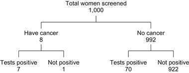
The first example is about false positives in breast cancer screening. The probability of breast cancer among women is generally estimated as .008, and the likelihood of a positive reading, given that a woman does have a cancer, is .90. This is a scary number for someone who has just had a screening and is told that the mammogram was positive for cancer. But wait a minute. What is really wanted here is a different conditional probability, namely, the likelihood of having cancer, given that the reading is positive. To understand this one needs to look at false positives, that is, the probability of a positive reading when the patient has no cancer. This is estimated to be .07. Let’s see where this leads us. Consider, say, a thousand women who undergo a screening. Of these, eight have cancer; of these, seven test positive. This leaves 992 women, of whom approximately 70 test positive (the false-positive rate); therefore, 922 have a negative result. Altogether, then, about 77 (that is, 7 + 77) out of 1,000 test positive for cancer, but only 7 actually have the disease, as shown in Figure 5.1. Consequently, the probability of having cancer, given a positive mammogram, is 7/77 = .09. It turns out that what at first glance seemed like a 90% chance of being diseased is actually a much lower 9%, or, to state this differently, approximately 9 out of 10 women who test positive do not have cancer. Indeed, the bulk of the tested women do not have the disease, and so, even though the chance of a positive reading is low, their sheer numbers means that a significant number of them will test positive. A more formal, but less revealing, derivation of the same conclusion can be based on Bayes’ Theorem, as we will show in the next section.
I turn now to a misreading of data known as the Prosecutor’s Fallacy. Using a hypothetical example, suppose that a DNA sample of a murder suspect is found to match that of the victim. The prosecutor is informed by an expert witness that the probability of such a match is roughly .0001. Let I denote “the suspect is innocent” and D the evidence “DNA samples match.” Because the probability of D is tiny, the prosecutor concludes that the suspect must be guilty, since it is otherwise very unlikely, given the match, that he be innocent. The prosecutor is confounding here the probability of a match with the probability that the suspect is guilty given that there is a match. However, what is really wanted here is prob (D|I), the likelihood of a match when the suspect is innocent. The fallacy is that the populations of people whose DNA match and of those who are innocent are vastly different in size, much as in the case of the probabilities of breast cancer that was just discussed. If the suspect resides in a city of 100,000 people, let us say, all but one of whom are considered innocent, then we would expect about 100,000 × .0001 = 10 individuals whose DNA profiles match that of the victim, and only one of them can possibly be guilty. That is, then, in the absence of any other incriminating evidence, the suspect has a 1 in 10 chance of being the murderer, and so his probability of innocence is .9, namely, prob(I|D) is about .9.
Similar considerations apply in other, less familiar, settings. In Section 5.3 we consider a very specific example of colorectal screening based on a study published in the New England Journal of Medicine; in Section 5.4 we take a look at the celebrated murder trial of former football star OJ Simpson, in which his defense attorney applied fallacious reasoning.
There is an aspect of Bayes’ Theorem that needs to be underscored: the effect that new evidence has on prior assumptions. Although this is implicit in each of the examples given so far and in all the ones to follow, it is important to bring this attribute of conditional probability into sharper focus. This we do in Sections 5.5 and 5.6, citing examples from sports to psychology to the testing of drugs. In preparation for this I consider briefly here the story of the well-known fund manager Bill Miller of the Legg Mason Fund, who, starting in 1991, was able to beat the S&P market index for 15 successive years. It should be said, however, that even though the likelihood of getting a success run like Miller’s by chance alone is small, if you believe that a fund manager is especially clairvoyant and perceptive, you should certainly invest with him or her during one of his or her success runs.
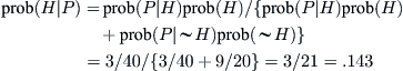
To bolster this conclusion I apply Bayes’ Theorem. Suppose you know that one of a group of coins is biased in favor of coming up heads during a toss. You watch the coins being flipped for a while and then ask for the probability that some particular coin is the favored one, given that it just came up heads. There is an analogy here between the coins outcome and the monthly performance of a select group of fund managers that seem to be good candidates for success, meaning, as usual, that they can outperform the S&P index of stocks. Let H be the hypothesis that some particular coin (fund manager) is biased (above-average performer) and P be the event that a coin turns up head when tossed. To be specific, assume there are ten coins, nine fair and one biased with a probability of 3/4 of coming up heads. The conditional probability that a particular coin will come up heads among the group of coins being tested satisfies prob(P|H) = ¾, whereas prob(P|∼H) = ½, where ∼H indicates the negation, namely, the complement of H. You don’t know which coin is biased, and so the prior probability that any given coin will be favorably biased is prob(H) = 1/10. We want to find the conditional prob(H|P), since this constitutes the posterior probability that a given coin is biased after we perform an experiment and observe that this coin did in fact come up heads. Jumping ahead to the next section, we can apply Bayes’ formula (5.1) to find that prob(H|P) = .143.
Thus, a prior probability that a coin is biased has now increased slightly from .100 to .143, given that the coin actually came up heads and assuming that at least one of the coins is biased. In reality there are perhaps several thousand potential fund managers, a very small percentage of whom have the ability to beat the market for a sustained period of time. The others are like fair coins and outperform or underperform the market with the same frequency. The argument from Bayes’ formula tells us that it makes sense to track the ones who do well in successive months even though we cannot be certain who among them have the knack for being the ones who can beat the market. At the very worst (I’m ignoring management fees here) we have even odds of matching the actual market performance. Although a success run for a fund manager can be largely attributed to chance, in the sense that one cannot dismiss the likelihood that tossing a fair coin at each investment opportunity gives results that are consistent with actual performance, it does not say that a successful streak is not due to a special market insight on the part of the fund investor. If you had invested with Bill Miller early in his streak, making updated observations of better-than-average returns month after month, your prior doubt about his skill would lessen over time. Needless to say, since chance intrudes on skill, an increase in the variance of market conditions may result in curtailing the streak of good fortune by a regression to mediocrity, as can be expected whenever there is an interplay between skill and luck. Since the financial turmoil that began in 2007, Mr. Miller had been on a losing streak, and in 2012 he finally stepped down from Legg Mason. Similar comments apply to other legendary stock pickers, like Peter Lynch of Fidelity Magellan Fund with a decade of success, and the same holds true for outstanding baseball players, as will be discussed further in Chapter 6.
5.2 Bayes’ Theorem
Suppose we are told that in two tosses of a fair coin at least one of them was a head. This narrows the sample space to event B, consisting of HH, HT, TH, since TT is no longer a possibility. Let A be the event that the other toss also was a head, namely, that HH took place. The conditional probability of A given B is now 1/3. Conditioning is a tricky notion that easily leads to unanticipated results, as will see throughout this chapter, and Bayes’ Theorem, to be discussed shortly, plays an essential role in clarifying this idea.
I begin with a review of some simple probability leading to Bayes’ Theorem. If we are given a sample space S and an event B ⊂ S that is known to have occurred, all future events must now be computed relative to B. That is, B is now the new sample space, and the only part of event A that is relevant is A ∩ B. Defining the conditional probability of A given B, written as prob(A|B), as a quantity proportional to prob(A ∩ B), it is easy to see that the constant of proportionality must be 1/prob(B) in order that prob(B|B) equal 1. Thus,
![]() (5.1a)
(5.1a)
or, equivalently, since it is also true that prob(B|A) = prob(A ∩ B)/prob(A),
![]() (5.1b)
(5.1b)
Sometimes it is convenient to write the denominator in (5.1) in a different way. To do this, note that the sample space S can be written as a union, S = A ∪ ∼A, where, as already noted, ∼A means the complement of A. Then B = B ∩ S = B ∩ (A ∪ ∼A) = (B ∩ A) ∪ (B ∩ ∼A). This last identity is easily established by showing that each side is included in the other.
Since A ∩ B and A ∩ ∼B are disjoint events, it now follows that prob(B) = prob(A ∩ B) + prob(A ∩ ∼B) and, using (5.1), we obtain
![]() (5.2)
(5.2)
Combining (5.1) and (5.2) provides one form of what is known as Bayes’ Theorem:
![]() (5.3)
(5.3)
To illustrate (5.3) we return to the question of false positives in breast cancer screening that was discussed in the previous section. Let U denote the event of a positive reading and V the event that a woman has breast cancer. Then
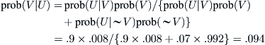
which is close to the value of .09 obtained by a less formal argument in the previous section.
For the sake of completeness I also apply a formal Bayes’ computation to the coin-tossing/fund manager problem treated in the previous section:
I remind the reader that event A is independent of event B if the conditional probability of A, given B, is the probability of A itself, which paraphrases the idea that the knowledge that B has occurred has no influence on the likelihood that A will take place. From (5.1) we see that A is independent of B if and only if prob(A ∩ B) = prob(A)prob(B), and this product rule extends to N independent events.
I digress briefly to discuss an alternate way to express chance. Suppose that the sample space is finite and consists of n equally likely outcomes, each of which has probability 1/n. In this setting, the probability of an event A is the number of ways A can occur (favorable outcomes) divided by the total number of possible outcomes. The odds of A is the number of ways A can occur (favorable outcomes) divided by the number of ways it cannot occur (unfavorable outcomes).
Thus, if A consists of m outcomes, then prob(A) = m/n, and odds(A) = m/(n – m). Since prob(∼A) = 1 – m/n = (n – m)/n, it follows that odds(A) = prob(A)/prob(∼A). Conversely, given the odds as a ratio m/(n – m), then prob(A) = m/(n – m + m) = m/n.
For example, a jar contains 6 red, 12 white, and 12 blue marbles. The probability of pulling out a white marble by chance is 12/30 = 4/10. However, the odds of a white marble is 12/18 = 2/3. Another example is that even odds of 1/1 is equivalent to a probability of 1/2.
Formula (5.1) tells one that the factor prob(E|H)/prob(E) represents the effect that the evidence E has on our prior belief in the hypothesis H. In terms of odds instead of probabilities, this is usually expressed as posterior odds = prior odds × BF. More precisely,
![]()
where BF is the so-called Bayes’ Factor: prob(E|H)/prob(E|∼H). Thus
![]() (5.4)
(5.4)
5.3 Colorectal Screening
Two separate studies on the effectiveness of colonoscopy were published together in the July 2000 issue of the New England Journal of Medicine (volume 343, pp. 162–208). Together they provide a quintessential Bayesian moment, as I’ll now describe.
More than 5,000 individuals underwent colonoscopies in the combined investigations, with the goal of determining the extent to which polyps in the lower colon (those parts of the rectum and colon that are reachable by a sigmoidoscopy) were or were not indicators of advanced lesions in the upper colon (which can be reached only with a full colonoscopy).
The conclusions reached in both studies were consistent: A significant percentage of people with advanced lesions (adenomas) or cancerous polyps in the upper colon would not have had the disease detected had they relied solely on a sigmoidoscopy (51% in one study and 46% in the other). Therefore, in spite of the considerable cost, the inconvenience, and a slight risk of procedural complications, the investigators recommended a full colonoscopy (a finding that was underscored in the New York Times, July 20, 2000, by Denise Grady [58] called “Broader, and More Expensive, Test Needed to Spot Colon Cancers, Studies Say.” From my discussions with several gastroenterologists it appears that these findings have altered their practice in the decade since the report from one that relied primarily on the simpler and less expensive sigmoidoscopy to the now-routine recommendation of a full colonoscopy for the majority of their patients.
There is, however, another conclusion to be drawn from the same data that at first glance almost seems contradictory: of all individuals showing no lesions in the lower colon (more than half of all those examined), only a small percentage will actually be found to have advanced upper colon disease (27 out of 1,000 in one study and 15 out of 1,000 in the other). This speaks in favor of a sigmoidoscopy alone.
This can be explained quite simply by looking at the bottom line of the data reported in studies I and II (I use the medical terms distal and proximal for lower and upper colon, respectively, in which distal includes the descending colon):
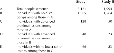
Now observe that the probability of advanced upper colon lesions, given that there are no lower colon polyps, is approximately the ratio of D to B, namely, 48/1,765 = .027 in one case and 23/1,564 = .015 in the other.
On the other hand, the probability of no lesions in the lower colon, given that there is advanced upper colon disease, is approximately the ratio of E to C, namely, .51 in one case and .46 in the other.
Although these assertions sound superficially alike, they are not the same. Let U denote the event that there are advanced proximal lesions and L that there are no distal lesions. The fallacy lies in confusing the probability of L given U with the probability of U given L. What has happened is that the population of individuals with no distal lesions is quite large, and only a relatively small number of these manifest serious lesions in the upper colon; by contrast, the number with serious upper colon disease is a relatively small fraction of the total population, but these include a fairly large percentage of people with no polyps in the lower colon. The underlying sample populations for the two statements are therefore quite different, a fact that is the source of some confusion in statistical reasoning in general, as you have already seen and will continue to see in this and the next chapter.
A simple self-explanatory diagram captures the entire argument in a nutshell, as we see from Figure 5.2.
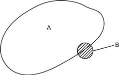
FIGURE 5.2 A is the set of people with no polyps in lower colon, and B is the set of people with upper colon lesions.
From the point of view of a physician, it makes sense to behave with caution and to quote the second statistic to a patient, recommending a full colonoscopy, since “about 50% of all cancerous polyps (in the upper colon) would not have been found from a sigmoidoscopy alone.” This is good advice and is entirely correct as a statement. But this needs to be reconciled with what a patient (with no family history and trying to avoid the discomfort, risk, and considerable expense of a colonoscopy) states, in an equally correct manner, that “if a simple sigmoidoscopy shows no polyps, then there is only a very small chance that my upper colon will exhibit any cancerous lesions.”
Based on the data, both statements are true. But when I tried to explain this to my own gastroenterologist, he insisted, with some irritation, that the first statement is the only relevant one, disregarding the second.
Incidentally, Bayes’ rule tells us that prob(U|L) should be identical to prob(L|U) prob(U)/prob(L). It is straightforward to verify that this relation does in fact hold exactly using data set II from the foregoing table and approximately in the first set (not unexpected, since the data is just a sample from a larger, unknown population).
A similar story can be found in terms of the less sensitive hemoccult test to check for blood in the stool. In a book by Gigerenzer [52], we read that about 30 people in 10,000 have colorectal cancer, a figure that is not totally at odds with the numbers available from the foregoing studies (in study II, for example, it was found that 12 of the people out of the 1,994 people studied had cancer). Of these, about half test positive, namely, 15 out of 10,000. Of the remaining 9,970 people with no cancer, some 300 will still test positive, so a total of 315 individuals test positive. The probability of having cancer given a positive test is therefore 15/315 = .048. Once again, the test is misleading. And, again, this conclusion is consonant to what we already know, namely, that when a disease is rare, as in the case of colorectal cancer, the number of true positives will be low and most positives will be false.
5.4 Murder and OJ Simpson
I mentioned earlier that prosecutors in a trial can argue erroneously. The same applies to the defense. An example of this was provided by the noted attorney Alan Dershowitz, who was part of the team working on behalf of OJ Simpson’s defense in the celebrated 1995 trial, in which Simpson stood accused of murdering his wife, Nicole. He was known to have physically abused her in the past. In a Los Angeles Times article from January 15, 1995, Dershowitz claimed, somewhat correctly, that in the country at large there is less than a one in a thousand chance that a woman abused by her current or former husband or boyfriend (let’s call such an individual her mate, for short) is actually murdered, and therefore Simpson’s past history is irrelevant. If G denotes the event that a woman is murdered by her mate and Bat is the event that the defendant has abused his mate, then what Dershowitz is saying, in effect, is that prob(G|Bat) is less than .001. Moreover, it is known that of the 4,936 women who were murdered in 1992, about 1,430 were killed by their mate, so the prior probability of G is prob(G) = .29. So not only is it not important that Simpson abused his wife (since only one in a thousand abusers goes on to kill), but the likelihood that he is the murderer, all other evidence aside, is not large enough for guilt.
This argument can be rebutted using the odds version of Bayes’ formula (5.4), in which H is the hypothesis that we now label G, namely, the event that a male defendant has murdered his mate. What is needed is prob(G|M and Bat), where M is the event that a male’s mate was actually killed by somebody.
In this computation, the “less than one in a thousand chance that a woman abused by her mate is murdered” is updated here to “1 in 2,500.”
To start, prob(G|Bat) = 1/2,500, and therefore the prior odds (G|Bat) = 1/2,499, which is roughly 1/2,500. Moreover, it is certainly true that prob(M|G and Bat) = prob(M|G) = 1. There were roughly 5,000 women murdered in 1995 out of a population of 110,000,000 women in the United States. It is known, moreover, that those women who were killed by someone other than their mate have the same likelihood of prior abuse by their mate as do women in general, and so prob(M|∼G and Bat) is about 1/20,000. The Bayes’ factor, BF, is therefore 20,000. Putting all this together gives the posterior odds that an abuser is guilty, given his wife was murdered, as
![]()
Transforming odds into probability [recall that prob = odds/(1 + odds)], we obtain prob(G|M and Bat) = 8/9. This is considerably higher than Dershowitz’s a priori estimate of .29, and, after acknowledging that a murder was in fact committed, it increases the plausibility that an abusive mate actually committed the murder. What all of this says about OJ Simpson I leave for you to speculate about.
The computation I just gave is based on a version of Bayes’ formula that is not overly familiar. However, there is a startlingly direct way to reach the same conclusion, which is illustrated in Figure 5.3. Here, for convenience, we look at the fate of 100,000 battered women.
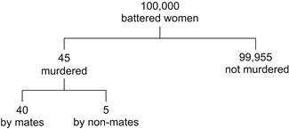
Bingo! In only one out of nine cases is the murderer someone other than the partner, and so the probability of guilt is, again, 8/9. (The number 45 was arrived at by recalling that only 1 battered woman out of 2,500 is killed annually by her mate, namely, 40 out of 100,000, while 5 out of 100,000 are killed by someone else, as we estimated earlier.)
An alternate argument that is also based on the odds formula and that uses the original “less than one in a thousand chance that a woman abused by her mate is murdered” estimate reaches a similar conclusion, namely, that the probability of guilt for an abusive mate lies between .67 and .86.
5.5 Skeptical Bayesians
It is helpful to understand the pretty much standard way of testing a hypothesis, as in deciding whether a novel treatment or drug is effective in treating certain ailments or a new teaching tool is effective in teaching and how this can be seriously at odds with a Bayesian approach. The usual method goes something like this. You want to see if the difference between the outcomes of two experiments are really significant or if we are simply observing the effect of chance fluctuations that are always part of an investigation. For example, a drug is tested on two sets of humans who are as evenly matched as possible. Actually only one set gets the drug, whereas the other gets a placebo. The investigation is carried out as a double-blind, in which neither the investigators nor the participants know who got the actual drug. After comparing results, a difference is noted that you would like to attribute to the drug’s effectiveness. But you can’t be sure because, as we said, there is always some variability due to a number of unavoidable experimental errors and the limited size of the sample. So you set up a dummy hypothesis H, the so-called null hypothesis, that the differences one observes are due simply to random variation.
What we have now is almost a cookbook recipe. The null hypothesis H is the strawman of statistical testing, in that one usually attempts to show that it is improbable. The alternative, namely, the plausibility of ∼H, would be more problematic and so this approach is not used. This is because there can be many alternatives to H, and these are not always easy to pin down. If, for example, the drug–placebo experiment makes it unlikely that the results are due to mere chance, then what can one say—that the drug is marginally effective or very effective, or that some hidden bias was introduced in selecting the set of patients, or, perhaps, that the experiment was stopped too soon to be decisive, or . . . ?
In any case, we construct a measure of variation known as a statistic, call it S, that presumably is a good indicator of significance, one that can discriminate between sampling error and a real effect in the experiment. Assuming H, we compute the probability distribution F(x) = prob(S < x). Either F is known or it is necessary to simulate it by generating a large number N of random samples of S and then counting how many of these lie below x, divided by N. By the Law of Large Numbers, this gives us an estimate of the probability F(x).
Suppose that the actual data gives a value of S∗. We then find the p-value, namely, the probability of finding a value of S as large as S∗ under the null hypothesis; large values of S cast doubt on H. Since we are usually interested in the upper tail of the distribution, the p-value is prob(1 – F(S) > 1 – F(S∗)). If this p-value is less than some cutoff quantity α, known as the level of significance, then H is rejected and the experimental result S∗ is judged to be significant at the α level. The most usual values for α are .05 or a more stringent .01. Note, however, that a rejection of H at a significance level of .05, say, does not mean that there is only a 5% chance that the result is a fluke, nor does it imply that the experimental results are significant with probability .95. It simply says that the null hypothesis is untenable at the 5% confidence level using the particular test statistic.
So far, so good. That’s the background to the garden-variety statistical technique used by many, perhaps most, researchers in the social and psychological sciences and in much of the medical literature.
However, by now we are conditioned to expect a Bayesian to raise an objection. The preceding technique computes the probability of getting the experimental result S∗ given the null hypothesis, namely, prob(S∗|H). But isn’t prob(H|S∗) what we really want? These two quantities are generally not the same, and in many instances we may actually be underestimating the likelihood that H is true, in which case the effect we observe may be spurious or, at least, much less probable.
To put this in context, let’s consider a simple example. An alleged wine expert is given four wines to taste and is required to match these with a list of four specific and closely related wines. These samples could, for example, be from the same producer using different vineyard sites or from different producers in the same region who are using the same grape varietal. The wines are tasted blind, with no visual clues for the taster. To obtain a perfect match by chance alone (guessing or, equivalently, by tossing a fair coin) has a probability of 1/24 = .063. If, in fact, the taster does get a perfect score, then we tend to reject the null hypothesis of mere guessing at the .063 confidence level. However, suppose we have prior information about the taster that, although he is a certified sommelier, his reputation as having a discerning palate is not so good. To be fair to the taster, we take an evenhanded agnostic view that there is a 50-50 chance that he (or she) is bluffing (p = ½) and, to the contrary, is applying genuine expertise (which would imply ½< p < 1). We now use Bayes’ formula (5.3) in the form
![]()
with, as discussed in Section 5.2,
![]()
H is the null hypothesis that his or her judgment is no better than a shot in the dark, and D is the result of the actual tasting, namely, a perfect match. Using this formula we should be able to get a better estimate of how likely H is given the result of the tasting, knowing that the prior odds of H are 1 (that is, prob(H) = prob(∼H) = ½).
We have no way of determining the actual level of expertise of the taster, and so we average over all possible values of p from ½ to 1 to obtain prob(D|∼H) = (the integral of p4 from ½ to 1, which is roughly .20). Since prob(D|H) = .063, we find that the posterior probability prob(H|D) is about .24. So the evidence of a random choice by the taster has decreased by half, from a probability of .50 to .24, and, though this still provides some evidence that the taster was not bluffing, the conclusion is now not quite as compelling as the one we were led to infer by rejecting the null hypothesis H at the .063 level. This last number is nearly four times smaller than .24, and what began as significant evidence against H needs to be amended in view of the Bayesian computation; even with an agnostic prior, we underestimated the likelihood of the taster’s achieving a perfect match even if she/he is merely bluffing. Put another way, we may have overestimated the skills of the taster. Of course, there is a subjective element to this Bayesian inference that can make one uneasy about using it. Although the choice of prob(H) = prob(∼H) = ½ is a nice agnostic point of view, the choice of prob(D|∼H) is not always obvious, and it can affect the final value of H. Your initial belief changes the posterior odds.
Not weighing prior evidence becomes particularly troublesome when, for example, a pharmaceutical company is eager to topple a null hypothesis in favor of declaring that they have a successful new drug, or a medical lab is to hype a new therapy when it may be no better than a placebo effect. They may be sweeping under the rug any prior evidence that would make it more difficult to reject the null hypothesis. There is a natural bias in favor of rejecting the idea that a favorable outcome is due solely to chance, touting a false positive, whenever there is a strong financial motivation or some other compelling reason to report a positive finding.
To buttress these concerns, consider a recent take by Carey that appeared in the New York Times [28, 29] on a set of extrasensory perception (ESP) experiments. The experiments by Cornell psychologist Daryl Bern tend to support the idea of ESP, but this has been received with skepticism because of a high prior belief in the null hypothesis that ESP doesn’t exist. I quote from part of the article:
Claims that defy almost every law of science are by definition extraordinary and thus require extraordinary evidence. Neglecting to take this into account, as conventional social science analyses do, makes many findings look far more significant than they really are. Many statisticians say that conventional social-science techniques for analyzing data make an assumption that is disingenuous and ultimately self-deceiving: that researchers know nothing about the probability of the so-called null hypothesis. In this case, the null hypothesis would be that ESP does not exist. Refusing to give that hypothesis weight makes no sense, these experts say; instead, these statisticians prefer a technique called Bayesian analysis, which seeks to determine whether the outcome of a particular experiment “changes the odds that a hypothesis is true.”
It may be enlightening to see another example of this kind of inference playing a role in an unexpected place. I quote here from the introductory part of an article by Nate Silver [104] in the New York Times about the WikiLeaks founder Julian Assange that also gives a striking illustration of where Bayesian thinking can be used to advantage.
Suppose that you are taking the bullet train from Kyoto, Japan, to Tokyo, as I did yesterday. The woman seated across from you has somewhat unusual facial features. You are curious to know whether she is Japanese, Caucasian, or some mix of both. Suppose furthermore that I asked you to estimate, in percentage terms, the likelihood of each of these three possibilities (ignoring others like that she might be Korean, Latina, etc.). Certainly, there are lots of other clues that we might look for to improve our estimate: How is she dressed? How tall is she? What type of mobile phone is she carrying? What is her posture like? (The more forthright among us, of course, might also seek to start a conversation with her, in which case the answer might become clear more quickly.) That notwithstanding, in the absence of further information, most of us would tend to equivocate: Perhaps there is a 25 percent chance that she is Japanese, we might say, a 25 percent chance that she is Caucasian, and a 50 percent chance that she is of mixed ethnicity.
But that would be a fairly bad answer. Even in the absence of additional information about the woman, we have another very important clue that can become surprisingly easy to forget if we become too fixated on the details: We are in Japan! There are a lot more Japanese people in Japan than there are Caucasians (indeed, the country remains among the more ethnically homogeneous industrialized societies). It probably follows also that there are a lot more white-looking Japanese people in Japan than there are Japanese-looking white people. It’s therefore quite a bit more likely that we’ve encountered one of the former than one of the latter on our train ride. A better “prediction” about her ethnicity, then—conditioned on the fact that we are in Japan—might be something like this: There is a 60 percent chance she is Japanese, a 35 percent chance she is mixed, and only a 5 percent chance she is Caucasian. If we were on a train from Boston to New York, instead of from Kyoto to Tokyo, the probabilities would gravitate toward the other end of the spectrum. Psychologists and behavioral economists have conducted a lot of experiments along these lines, testing our ability to think through problems that involve what statisticians call Bayesian inference: those that require us to infer the likelihood of various possibilities based on a combination of prior, underlying conditions (we are in Japan: Most people we encounter here will be of Japanese ancestry) and new information (but, based on this woman’s appearance, it is hard to tell whether she is Caucasian or Japanese!). They’ve found that, in general, we do pretty badly with them: We tend to get lost in the most immediate details and we forget the underlying context.
Nate Silver then goes on to make an analogy with the charges brought against Julian Assange from the Swedish authorities that on face value have to do with accusations of rape but, because of his provocative leaking of government secrets, were more likely to be politically motivated.
5.6 Batting Averages and a Paradox
Because its solution is closely tied in with Bayes’ theorem, I want to discuss an idea that is seemingly paradoxical. Besides the intrinsic interest of this problem, there are other reasons for introducing this here since it is closely connected to two other statistical conundrums, the notion of regression to the mean and the surprising role of the variance of a sample mean. All of this will become clearer as we proceed, with some of the mathematical niceties postponed to Section 5.7.
We are given n independent random samples y1, . . . , yn from a normal distribution of unknown mean θ and unknown variance σ2, and we want to obtain a good estimate θ of this mean, in the sense that θ minimizes the expected squared error E(θ – θ)2. It turns out that the sample mean X = 1/n ∑ yj, summed over j, is the optimal maximum-likelihood estimator θ, as will be discussed in the next section. Note that this estimator is unbiased, in the sense that E(X) = θ, and so E(θ – X)2 is the variance of X. Observe, for later reference, that the variance of X is σ2/n.
Now to an unexpected result known as Stein’s paradox. Suppose that we have m separate and unrelated parameters θ1, . . . ., θm to estimate. Using the foregoing procedure, we form m sample means X1, . . . ., Xm using the same sample of size n for each and then form the measure of estimation error
![]() (5.6)
(5.6)
summed over k from 1 to m. One might think that this provides the best estimate for the m parameters together. Surprisingly, however, there is a better mean-squared approximation to the θ’s called the James–Stein, or JS, estimator when m exceeds 3. To discuss this curious property and in anticipation of some other bizarre consequences, I follow Efron and Morris [42, 43] and use a baseball example. Because baseball has a rich database of player statistics, this is an ideal vehicle to illustrate what’s involved.
The first 18 Major League Baseball players to have been at bat 45 times in 1970 is given in the table presented shortly. For each player we compute the batting average BA (number of hits/number of times at bat), which is a sample mean based on 45 observations. I now show that the mean-squared error (5.6) can be improved by replacing Xj for the jth player by a quantity Zj, defined by
![]() (5.7)
(5.7)
where X is the average of all the individual averages, namely, X = 1/m ∑ Xk, and c is a constant, to be specified later, that is less than 1. The idea behind c is that it serves to shrink each of the individual sample averages toward the grand mean X so that high performers in the preliminary 45 at-bats have their batting estimates reduced somewhat while low performers are increased. This regression to the mean X is meant to compensate for the fact that, though an early high performer may be just that, a consistently talented ballplayer, it is also possible that he was on a lucky streak. Similarly, a poor performer early in the season may be just poor or simply in an unlucky early slump. Only the rest of the season can tell.
If one takes the batting average over the remaining season (about nine times more data is now available than from the preliminary estimate of over 45 at-bats), this becomes a good estimate of the actual players’ performance during the season, since the variance of the estimate tends to zero with the number of samples, and we designate this season-wide average as θj and use it as an approximation to the true but unknown mean θj for the jth player. In the present case X has the value .265. The top hitter in the league in 1970 was Roberto Clemente, who achieved a batting average of .400 in the beginning of the season (45 at-bats). Using a value of c that is discussed further later, we get for his revised average the value .265 + c(.400 – .265) = .290, which is a worse reflection of his true ability than found by the season mean of .346. However, this happened in only three cases, and for 15 of the 18 players the JS estimator of their batting averages gave a better individual mean-squared error (see the upcoming table, in which BA is the batting average and AB is the number of at-bats). The comparison was achieved by computing the value of (5.6) using Xj in one case and the value of the JS estimator Zj in the other. In one case, using the X values, the aggregate value of (5.6) is .077, whereas with the JS estimator the value is only .022, a ratio of 3.5 to 1.
After each player’s name in the following table, the first column is the value of the sample mean X, namely, the batting average for the first 45 at-bats. The second column is θ, the season batting average, and the last column is the corresponding JS estimator.
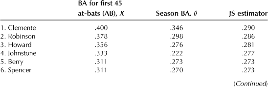
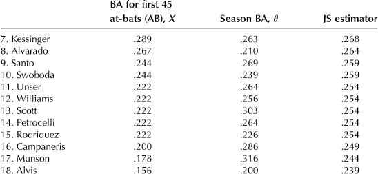
We begin to see a problem here. To quote Efron and Morris [43], “What does Clemente’s .400 observed average have to do with Max Alvis, who was poorest in batting among the 18 players? If Alvis had had an early season hitting streak, batting say .444 instead of his actual .156, the JS estimator for Clemente’s average would have been increased from .290 to .325. Why should Alvis’ success or lack of it have any influence on our estimate of Clemente’s ability? (They were not even in the same league.)” But it gets worse. The initial assumption is that the θ values were unrelated. So why do we limit ourselves to just baseball, in which all these values are relatively close to each other? Let’s include some other data, say, the weights of 45 randomly chosen candy bars. The average of these weights is an estimate of the true weight. But another approach is to lump this value in with the averages of the 18 players. Or, to use another example (Efron and Morris [43]), a random sampling of automobiles in Chicago finds that, of the first 45, 9 are foreign made and the remaining 36 are domestic. This gives an observed average of .200 as the ratio of foreign cars. Suppose this single average is lumped in with those of the 18 players. Now we have 19 θ values, which changes the grand average, and, as will be seen, the value of c is altered slightly and the JS estimate for the cars is now increased to .251. To quote again from Efron and Morris [43]:
In this case intuition argues strongly that the observed average and not the James–Stein estimator must be the better predictor. Indeed, the entire procedure seems silly: What could batting averages have to do with imported cars? It is here that the paradoxical nature of Stein’s theorem is most uncomfortably apparent: The theorem applies as well to the 19 problems as it did to the original 18. There is nothing in the statement of the theorem that requires that the component problems have any sensible relation to one another.
As one exasperated commentator put it, in an article about Stein’s paradox: “That sounds like it’s just plain nuts” (Birnbaum [20]).
Let’s look at this closely, leaving out the nitty-gritty details since an alternate approach using Bayes’ Theorem will be given shortly. It turns out that a wide variability in disparate components has the effect of making c approach unity, and so little or no shrinkage occurs. Conversely, when the means are tightly clustered, the shrinking factor becomes more pronounced. Thus, throwing in candy bars and automobiles or wheat production figures with baseball has the effect of increasing c, and the overall effect of the JS estimator becomes more negligible. To quote, for the last time, from Efron and Morris [43], “In effect, the James–Stein procedure makes a preliminary guess that all the unobservable means are near the grand average. If the data supports that guess in the sense that the observed averages are not too far from Y, then the estimates are all shrunk further towards the grand average. If the guess is contradicted by the data, then not much shrinkage is done.”
Although (5.6) improves when averages are replaced by the JS estimator, this does not mean, as we saw in the case of Roberto Clemente, that every individual component gets a better estimate. It is the mean-squared average over all components together that improves. The implication is that more than enough components get better estimates to compensate for the few who don’t. Individuals are sacrificed to the greater good, so to speak.
In an attempt to clarify what is going on, I will bypass a derivation of the JS estimator and turn instead to Bayes’ Theorem to help us out. We have, in the baseball example, some prior information that can be used to advantage, namely, that the batting averages of all the Major League players follow a normal distribution, which in 1970 had a mean of .270 and a standard deviation of .015. Put in a slightly different way, the unknown seasonal means θj of individual players are arranged according to a normal distribution with mean μ = .270 and standard deviation τ = .015. The normal density with parameters μ and τ is a distribution of batting averages that is prior to having made the observations of sample means X. In Section 5.7 it is shown that the posterior value of θj given the observed data is also normally distributed, with a mean that is the same as (5.2) but with X replaced by the prior mean μ of θj and the constant c now equal to τ2/(1 + τ2), in which τ = .015. In the present instance, therefore,
![]() (5.8)
(5.8)
This estimate has the same form as (5.7) and, centered as it is on Bayes’ Theorem, effectively predates the JS estimator by more than two and a half centuries, except JS has the added virtue of being independent of any prior belief about the true mean.
Writing E(θj|Xj) as Yj for simplicity, we can make the comparison between Xj and Yj more explicit in terms of the mean-squared error (5.1). It was already noted that the sample means Xj have a variance of σ2, and so the sum (5.1) becomes mσ2, since the samples are independent random variables. It is convenient to normalize the variances such that σ = 1, so (5.1) is simply m. However, when (5.1) is computed using (5.3), namely, Yj, we obtain (as shown in the next section) the value mτ2/(1 + τ2) < m, and so the Bayes’ estimator is an improvement over the maximum-likelihood estimator for any value of m. To see this more clearly, suppose μ = 0 and τ = 1. Then Bayes’ estimate shrinks the ordinary estimate by half toward the true mean of zero, since, in this case, τ2/(1 + τ2) = ½. Note that when the variance is large, very little shrinkage actually takes place, which confirms what we stated earlier regarding the JS estimate.
5.7 A Few Mathematical Details
We begin with the fact that if X1, . . . , Xn are n independent random variables from a normal distribution having unknown mean θ and standard deviation σ, then θ = θ(X1, . . . , Xn) is an optimal estimate of θ in the mean-squared sense if it minimizes the expected value
![]() (5.9)
(5.9)
In Appendix A we learn that θ is actually the sample mean (1/n) ∑ Xj = X, with j summed from 1 to n, and, since E(X) = θ, the expression (5.6) is the variance of X. Because the variables X1, . . . , Xn are independent, the variance of X = (1/n) ∑ Xj = (1/n2)∑ σ2 = σ2/n.
In Appendix A we find that the sample mean is also a maximum-likelihood estimate of θ; what this means is also explained there.
It is a convenient shorthand to write X ∼ N(θ, σ2) to mean that a random variable X is normally distributed with mean θ and standard deviation σ. Now suppose that θ itself is N(μ, τ2), and think of it as the prior distribution of θ before any additional information is available. What can we say about the value of θ given that we know the value of the sample mean X, written as θ|X, namely, when X = X? That is, I want to know the posterior value of the distribution of θ given the value of the sample X. From now on, the variance of X is assumed to have been normalized to a value of 1 by a suitable change of variables. Bayes’ Theorem then comes to our rescue, and in Appendix A we learn that (θ|X = X) is again normally distributed with mean
![]() (5.10)
(5.10)
and variance
![]() (5.11)
(5.11)
The computations that follow require the notion of conditional expectation (see Appendix D).
Expression (5.7) is Bayes’ estimate of θ given the information X, and if we compute E(E(θ|X) – θ)2 with respect to the range of possible X values in N(θ, 1), we obtain, letting w = τ2/(1 + τ2), E(μ + w(X – μ) – θ)2 = E(μ(1 – w) + wX – θ)2 = E(μ2(1 – w)2 + 2μ(1 – w)(wX – θ) + (wX – θ)2) = (μ2(1 – w)2 – 2θμ(1 – w)2 + (1 – w)2θ2 + w2), in which we have used the facts E(X) = θ and Var(X) = E(X2) + θ2. Thus, the expectation with respect to X reduces to
![]() (5.12)
(5.12)
in which, again, Var(θ) = E(θ2) + μ2.
Now take the expectation of (5.9), this time with respect to θ, to get, since E(θ) = μ and Var(θ) = τ2,
![]() (5.13)
(5.13)
It is appropriate that (5.13), namely, the expectation with respect to θ of the expectation with respect to X, is the same as (5.11), since the latter is the variance of E(θ|X), in which X takes on the specific value X, namely, the expectation with respect to θ of E(θ|X).
One last comment is that, roughly speaking, the Central Limit Theorem allows us to see (we will elaborate in Appendix A) that |X – θ| decreases with n as σ/√n, or, equivalently, |∑ Xj – θ| increases with n as σ√n. We will use these facts in the next section.
5.8 Comparing Apples and Oranges
Reversion to a population mean is one useful lesson we take away from the discussion in Section 5.6, namely, the idea that if a random variable is extreme in its first measurement, it will tend to be closer to the average on the second measurement. This is especially true for sample means, which tend to cluster about the population mean for large sample size but are more variable for smaller sample sizes. Extreme-tail events are less likely than values near the mean, and the likelihood is that most samples will revert to values closer to the center, what some call “reversion to mediocrity.” This is especially true when the variables are a measure of an individual’s performance in which there is an interplay between skill and luck, as in the examples given earlier of the batting averages of baseball players. An unusually high score now is more likely to be followed later by a lesser achievement as chance intrudes to swamp the effect of skill. A physician that is evaluated by some index of patient care, for instance, has his or her performance measured against the average score for all physicians. Observing a high-quality doctor can mean that this practitioner is actually a high-caliber professional, but it can also mean that the doctor is really mediocre but just happened to perform above average on some group of patients. By the same token, an inferior performer can be just that, inferior, or an average practitioner that happened to score poorly on the patients in the sample. Sooner or later we expect both extremes to shrink to the group average. A more mathematical take on this, at least for normally distributed variables, is discussed in Appendix A.
In our discussion of the James–Stein paradox, we saw that combining data sets from widely different populations can yield surprising results. I want to introduce here yet another conundrum of this type since it is closely related to the use of sample means, as in the aforementioned paradox, and because it further illuminates the idea of regression to mediocrity. I follow Wainer [113] by looking at all cases of kidney cancer in the United States, counted at the local level in order to obtain county-by-county incidence rates for purposes of comparison. Now consider those counties with the lowest 10% of cancer incidence. I quote: “We note that these healthful counties tend to be very rural, Midwestern, Southern, or Western. It is both easy and tempting to infer that this outcome is due to the clean living of the rural lifestyle—no air pollution, no water pollution, access to fresh food without additives, and so on.” Now one looks at those counties with the highest decile of cancer incidence, many of them adjacent to those healthiest 10%, and we read, “These counties belie that inference since they also tend to be very rural, Midwestern, Southern, or Western. It would be easy to infer that this outcome might be due to the poverty of the rural lifestyle—no access to good medical care, a high-fat diet, and too much alcohol and tobacco. What is going on?” The answer can be found in the normal distribution of the sample mean (see Appendix A), in which the cancer incidence rate differs from the overall population mean for the county by a factor of σ/√n, where n is the population size of the county. Rural counties with small populations have a greater variability in their means than larger regions. Again, “A county with, say, 100 inhabitants that has no cancer cases would be in the lowest category. But if it has one cancer patient it would be among the highest. Counties like Los Angeles, Cook, or Miami-Dade with millions of inhabitants do not bounce around like that.” In fact, the actual data shows that when county population is small there is a wide variation in cancer rates, from 0 to 20 per 100,000 people; when county populations are large there is little variation, with about 5 cases per 100,000 for each of them. Moreover, the number of cancer cases does not grown proportionally to n but, rather, to its square root, so, for example, the increase in the number of cancer cases in a county of 10,000 people varies by about 100, which is only 10 times more than a county with just 100 people. To put this in context, let’s consider a hypothetical situation of 100,000 people where two dogged individuals measure the sample means of some normally distributed attribute of these people, such as weight or height. If person A chooses to sample in batch sizes of single individuals and B in batches of 1,000 people, then in the first case we would see a highly variable spread of attributes, whereas B would see sample means clustering about the mean of 100,000 people and there would be little variability. The same considerations apply to comparisons of the mortality rate of hospitals of differing sizes or the college admissions rate of small versus large schools. Small schools appear to be overrepresented among those with the highest scores of academic achievement, which suggests breaking large schools into smaller ones. The problem is that the same data shows that underachieving schools also come from the pool of small schools, and, on average, large schools perform better than the smaller ones. In [113] we read that about a decade ago the Bill and Melinda Gates Foundation made substantial contributions to support smaller schools but that by 2005 the foundation decided to move away from this effort, citing better ways to improve effectiveness. There is a connection here with the regression to the mean, since a small school or small hospital that performs especially well on a year-to-year basis does so by a mix of competence and chance, and, because of the higher variability of small versus larger institutions, we should expect, as in the case of cancer rates discussed earlier, to see the same school or hospital perform less well in future years. This mix of skill and luck is also telling in the case of athletes and fund managers, as we have already seen and as will be discussed further in Chapter 6. For example, although most fund managers may beat the S&P stock index monthly for several months in a row (just as a fair coin may reveal several heads in a row when tossed), we expect there to be an eventual regression to mediocrity except for that very small group of investors with truly exceptional stock-picking skills whose performance streak can be sustained for a more extended period until they too are thwarted by chance events, as eventually happened to the celebrated Bill Miller in 2007 and 2008.
As another illustration of the pitfalls of mixing large and small data sets (mixing apples and oranges), consider the phenomenon known as Simpson’s paradox, which is concerned with a class of problems in which ranking second in successive periods can result in ranking first when the two periods are combined.
A real-life example of this type comes from a medical study comparing two treatments, A and B, for kidney stones. The success rate (successes per number of treatments) was 273/350 = .78 for treatment A and 289/350 = .83 for treatment B, indicating that B is more effective than A. However, the kidney stones can be grouped into small and large, and if one looks at these separately, one gets the following table, showing an inversion of the grouped ranks.
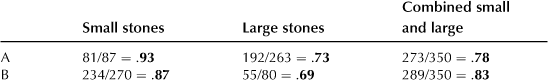
The mix of data for small and large stones is a central feature in the paradoxical switch in ranks, but other contributing factors are certain confounding variables that lurk behind the data. In the present case it turns out that the less invasive treatment, B, was used more often on small stones, where the treatment is generally more effective than it is on large stones. Overall, however, the more invasive traditional surgery always gives better results than the less invasive procedure.
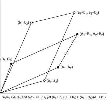
A nice pictorial explanation of how the paradox can arise is based on a simple vector space approach in which a success rate a/b is represented by a vector (a, b) in R2 having slope b/a. If two rates a1/a2 and b1/b2 are combined, the sum is represented as the sum of vectors (a1, a2) and (b1, b2) and is (a1 + b1, a2 + b2) having slope (a2 + b2)/(a1 + b1). A similar relation holds if a, b are replaced by A, B (see Figure 5. 4, taken from Kocik [72]. The paradox consists in the reversal of inequalities.
The bottom line to this entire discussion is that if we go looking for a pattern, the odds are good that we will find one. And small sample sizes only make it that much easier.
5.9 Concluding Thoughts
Additional details about choosing a better-than-average money manager, which was discussed in the opening section, can be found in an article by Hulbert in the New York Times [65].
I recommend a nontechnical book on the history of Bayes’ Theorem over the last two and a half centuries, written by McGrayne [80].
Without a doubt, Gigerenzer’s book [52], especially pp. 45–46 and 107–108, offers great insight into understanding the workings of Bayes’ formula in medicine (false positives and the effectiveness of hemoccults) and fallacies in courtroom proceedings, both of which I followed closely in my own treatment. The discussion of colonoscopies in Section 5.3 appears in print here for the first time.
The Bayes’ analysis of OJ Simpson’s probability of guilt follows I. J. Good [55] and Merz and Caulkin [82]. It is interesting to note that Alan Turing (discussed in Chapter 11) applied the odds formula in the statistical analysis he performed during the Second World War at Bletchley Park while working on the notorious Enigma code (See I. J. Good [54]) except that he worked with the logarithms of the odds to obtain what Good calls “the weight of evidence in favor of H provided by E.” Turing also called the BF simply “the factor in favor of a hypothesis” and, according to Good, who was Turing’s assistant at that time, this term was first introduced by Turing (without the qualification “Bayes”). Good also uses the evocative term “intelligence amplifier” to describe the logarithmic ratio of the posterior odds to prior odds.
The Prosecutor’s Fallacy is especially relevant in “cold-hit” files, in which an old unsolved murder case is revived many years later using remnants of DNA evidence that was gathered during the initial investigation. Most of the reliable witnesses from the past are by now dead or unavailable, and what remains are meager fragments of circumstantial evidence, so if someone is found with a partial DNA match, a prosecutor is likely to charge this individual with the crime. Contrary arguments to negate this fallacy are usually deemed to be inadmissible in a court of law, for a number of reasons (see, for example, “DNA’s Dirty Little Secret” by M. Babelian in the Washington Monthly, March/April 2010).
An informative discussion of faulty inferences using traditional statistical arguments is by Matthews [78,79].
That the JS estimator does considerably better than the averages in terms of (5.6) is based on work done by Charles Stein in 1956 and by James and Stein in 1961 in an article that appeared in the Proceedings of the Fourth Berkeley Symposium on Mathematical Statistics and Probability, pp. 361–379, and called “Estimation with a quadratic loss.” We follow the treatment in Efron and Morris [42,43]. Wainer’s article [113] has a number of interesting examples of the misconceptions that arise because the variance of a sample mean varies with population size.
The colonoscopy example of Section 5.3 has an added twist in terms of prior and posterior probabilities. The a-priori probability of proximal disease in Study I is simply the ratio of B to A, namely 128/3121 = .041. But if one now performs a sigmoidoscopy that reveals no distal polyps then, given this new information, the posterior probability of proximal disease decreases, as we have seen, to .027, which again supports the belief that a negative sigmoidoscopy is at least partially indicative of no proximal disease. A similar conclusion applies to study II.
The kidney stone example is taken from Julious and Mullee [68]. See also the short article by Tuna [111] reviewing various occurrences of Simpson’s paradox for the general reader.
For more insight into the use of Bayesian priors, see the provocative articles by Berger and Berry [18] and Berger and Sellke [17].
The colonoscopy example of Section 5.3 has an added twist in terms of prior and posterior probabilities. The a-priori probability of proximal disease in Study I is simply the ratio of B to A, namely 128/3121 = .041. But if one now performs a sigmoidoscopy that reveals no distal polyps then, given this new information, the posterior probability of proximal disease decreases, as we have seen, to .027 which again supports the belief that a negative sigmoidoscopy is at least partially indicative of no proximal disease. A similar conclusion applies to study II.
To close this chapter on the pitfalls of invalid inferences, I mention the very tricky business of correlated random variables in the context of an amusing example. In March of 2012, Representative Jeanine Notter of the New Hampshire legislature speculated aloud whether the use of birth control pills by women causes prostate cancer in men. This occurred at a hearing on a bill to give employers a religious exemption from covering contraception in health care plans (see “Politicians Swinging Stethoscopes” by Gail Collins, New York Times, March 16, 2012). In countries where the use of birth control pills has increased there appears to be a concomitant increase in prostate cancer, the implication being that there is a causal connection. It is one of the most common of statistical fallacies to mistake a correlation between two sets of variables with the idea that one variable is the cause of the other. There may be no connection at all. As the previously quoted New York Times article goes on to say, “You could possibly discover that nations with the lowest per-capita number of ferrets have a higher rate of prostate cancer.”