
What Are the Odds of That?
6.1 Background
The spooky quality of coincidences rarely fails to fascinate and confound people who experience them. A recent example was provided by former TV talk host Dick Cavett in his New York Times article of May 8, 2009, called Seriously, What Are the Odds?, which gave rise to the title of this chapter. Cavett was amazed that two people from different parts of the country came together and noticed that their individual automobile license plates were identical. Later, in another piece, called Strange, Dear, but True, Dear (Cavett, [30]), he continued with other tales of eerie happenstance.
What I hope to show in this chapter is that many, perhaps most, coincidences are less amazing than they first appear to be, with applications to a cross section of biological and social problems.
Sample spaces in probability contain all possible events and not just those that catch our attention. We tend to focus on those meaningful to us. In effect, when a coincidence appears that we happen to notice, what is being ignored here is the larger number of other events that also lead to striking coincidences but that we failed to detect. The source of wonder in an uncanny coincidence is our selectivity in picking those events that catch our fancy.
If you toss two identical balanced dice (a cube with sides numbered from 1 to 6), the sample space consists of 36 possible equally likely outcomes for the number of dots that appear on each die. We ask for the probability of getting the pair (3, 3). There is just one possibility here, and so the probability that this will happen is 1/36. However, if you ask for the probability that the same number will come up on each die, any number from 1 to 6, there are now six possibilities to consider: (1, 1), (2, 2), . . . , (6, 6), and so the probability that this event will occur is now 6/36 = 1/6. Asking for a particular coincidence is quite different from asking about any coincidence.
An interesting illustration of this in a lottery is described in the Montreal Gazette of September 10, 1981. The same winning four-digit lottery number 8092 came up on the same night in separate draws in the states of Massachusetts and New Hampshire, and the gambling official stated that “there is a 1-in-10,000 chance of any four-digit number being drawn at any given time, but the odds of its happening in two states at the same time are just fantastic.” Evidently they calculated the probability of the two independent events to be 10-4 multiplied by itself to give 1 chance in a 100 million. The fallacy in this conclusion is that the officials focused on the coincidence of the specific number 8092 instead of on the probability of matching any four-digit number, the probability of which is just 10-4, or 1 in chance in 10,000, just as in the toss of two six-sided cubes. Moreover, they didn’t distinguish between the occurrence of this event and of its occurring and being noticed. Since the two states are neighbors, the lottery results of both states are reported in local papers; but if the second state had been out west, it is less likely that the coincidence would have been noticed.
If one actually takes into account lotteries in multiple states, this would increase the odds of a coincidence even further. Another lottery example is that of a woman in New Jersey who won the lottery twice in a span of just four months. I will discuss this in more detail in a later section.
Selective reporting is a source of coincidences. To quote Cohen and Stewart [37], “The human brain just can’t resist looking for patterns, and seizes on certain events it considers significant, whether or not they really are. And in so doing, it ignores all the neighboring events that would help it judge how likely or unlikely the perceived coincidence really is.” Returning to Dick Cavett’s blog, he tells of casually glancing at a newspaper, during a vacation in the Hamptons, which announces a new Broadway musical. Walking on the beach later that day, he bumps into someone whom he doesn’t know but who appears to know him, and they start a conversation. To cover his embarrassment, Cavett mentions the new musical, calling it junk. The other person, to Cavett’s surprise, reveals that he is the author. But how many other opportunities were there for Cavett accidentally to meet someone of note? After all, both individuals are in the entertainment business, and vacationing in the Hamptons is not uncommon among affluent New Yorkers. Cavett could have met any number of acquaintances or near-acquaintances during his stay and, returning home, might later find that someone else he knew was also walking on the beach and that they had just missed each other. Then, too, the wealth of articles in the newspaper on a variety of topics provided him with ample opportunity to draw a connection with a large number of people in multiple related professions, one of whom he actually meets. But Cavett focused on a single chance encounter that he found embarrassing instead of considering the myriad other unplanned meetings that could have, and indeed may have, taken place that he didn’t deem important. As he ruefully observes, “I went home and looked up how many people there are in the world in a World Almanac. I could have run into any one of them. Couldn’t I?”
In a similar vein is the seemingly remarkable coincidence of birth and death dates of celebrated people. What comes immediately to mind are Jefferson and Adams, who died on the Fourth of July, 1826; Darwin and Lincoln, who were born on February 12, 1809; and Stalin and Prokofiev, both of whom died on March 5, 1953. There are many other examples. Consider this, however. In any one year there are many celebrities in the arts and sciences, and public life generally, who are born or die, and that the dates should coincide among any pair of them is not so striking. It is only when you focus on one particular pair instead of any pair that the concurrence appears remarkable. In the case of Adams and Jefferson, if you consider that there have been 44 presidents so far, a coincident birth date (or, if you wish, death date) has better than even odds (indeed, Monroe also died on July 4). Later in this section we show that the coincidence among some pairs of celebrities in one of the many different categories, such as movie stars, politicians and statesmen, authors, and so on, becomes even more likely as more categories are included, as long as we don’t focus solely on some specific pair of individuals.
A more quantitative spin on coincidence is carried out in the next section, followed by the mathematical details in Section 6.3. The Poisson distribution, which played so pivotal a role in Chapter 3 as a probabilistic tool for assessing how many events take place in space or time, returns in Sections 6.4 and 6.5 in a somewhat different guise in order to illuminate further the role of chance in coincidences as they occur in a wide number of social and biological settings. A valuable statistical technique is introduced in Section 6.6 to validate some of the results obtained in this chapter and because it is encountered frequently in biological modeling.
6.2 Coincidence and Near-Coincidence
To provide a guidepost to the phenomenon of coincidence, I consider first a generalization of the familiar birthday problem in which a group of k people are assembled quite arbitrarily and one inquires what the probability is that at least two of these individuals have the same birth date. Two modest assumptions are made here, which are not quite true, that all birthdays are equally likely to occur on any day of the year and that a year consists of 365 days. To make the problem more interesting, we extend this question to ask, in addition, what the probability is that at least two individuals have a birthday no more that one day apart (near-coincidence). I leave the proof of the following results to Section 6.3.
The probability that at least two of the k individuals share the same birthday is
![]() (6.1)
(6.1)
and the probability that their birthdays are no more than one day apart is
![]() (6.2)
(6.2)
When k is as small as 23, then (6.1) is greater than half and so there is a better-than-even chance that two or more of these 23 individuals will report the same birth date! On the several occasions on which I’ve tried this experiment in a classroom of about 30 students, only once did I fail to get an agreement on birth dates from two or more people in the class. The surprise here is that most students believe that it would require a much larger population of individuals to achieve such concordance.
The birthday problem may appear surprising because some people hearing it for the first time are responding to the wrong question, one that sounds superficially like the birthday problem, namely, “What is the probability that someone else has the same birthday as mine?” The real issue is whether any two people in a room have the same birthday, and there are many more possibilities for this to occur; we are fooled into thinking of the coincidence as something that happens between us and someone else rather than between any two randomly chosen individuals.
For the sake of demonstrating how different the probability that at least one of n randomly chosen people has the same birthday as myself, note that 364/365 is the probability that some particular person has a birthday different from mine; therefore, by independence, (364/365)n is the probability that none of the n people has the same birthday as I do. Consequently, the probability that at least one person does in fact have the same birth date as I do is 1 – (364/365)n. It takes n = 253 people before obtaining even odds of a match, and this number fits in better with the intuition of most individuals who first encounter the birthday problem.
Using (6.2), we find that there are now better-than-even odds that 2 individuals out of 14 will have the same birthday or a birthday one day apart. This shows (and verifies our intuition) that the likelihood of a close coincidence may be more common than is generally thought.
Near-coincidence, when it happens to us, is often seen as just as unsettling, but the odds that this will happen are even greater. When one of these people is yourself, the coincidence is striking, but, of course, there are good odds it will happen to someone. When it does, you either don’t see it or you don’t care. The phenomenon of my coincidence versus your coincidence has been examined through a set of psychological experiments that suggest that there is a real difference in the perception of how surprising an event appears depending on who it happens to.
In a national lottery, for example, in which a draw is 6 numbers out of the first 49, there are C(49, 6) = 13,983,816 possible outcomes, and a winning draw is a long shot for you. But out of the millions of people who play the lottery, many with multiple tickets, someone wins. And if your ticket differs from the winning one by just one digit, this may seem amazing. But, in fact, many people have tickets that differ from one another by a single number; however, because they don’t involve the winning draw, no one notices.
Another example may suffice to help us tame coincidence. A group of people meet and start to chat. Any number of quirky correspondences can now crop up. For example, two or more may share a birthday, or they may have attended the same university (at different times, however), they may have the same hobby, have grown up in the same neighborhood, worked at the same job, and so forth. What is the chance of a coincidence of some sort? To analyze this problem, I assume that each category of similarity is independent of any other category. With N people and k categories consisting of c1, c2, . . . , ck elements each, let’s find what N should be to ensure better-than-even odds that at least two people share some coincidence from one or more of these categories.
To carry out this computation I will use formula (6.12) from Section 6.4, which is based on the Poisson distribution. We find there that the probability of no coincidence among N people within a category of c elements (say, c = 365 birthdays) is e–N(N–1)/2c. For two independent categories this probability becomes e–N(N–1)/2c1e–N(N–1)/2c2, and 1 minus this quantity is therefore the probability p of at least one match. For an even chance that this will happen, we take p to equal ½ and then solve for N to see how many people this requires. Taking logarithms, it is easy to see that this leads to 0 = log 2 – N(N – 1)(1/c1 + 1/c2), and therefore, since the square root of log 4 is about 1.2, N is roughly 1.2 sqrt (1/(1/c1 + 1/c2)). For k categories this extends immediately to give
![]() (6.3)
(6.3)
For instance, if there are c1 = 365 birthdays, c2 = 500 same theatre tickets (on different nights), and c3 = 1,000 lottery tickets, then (6.3) shows that it takes only 16 individuals for an even chance of a match of some sort. We see, then, that multiple categories allow for the possibility of a coincidence with fewer people than one might expect. Note that with a single category of only birthdays, (6.3) gives an N of about 23, for a 50% chance of an even match, which agrees with the value obtained earlier.
For a final but informative example of a surprising coincidence, a variant of the previous problem, I borrow from a teaser posed in Tijms [109]. Two strangers from different walks of life happen to meet somewhere and begin to converse and, while doing so, discover that they both live in San Francisco, which has a population of roughly 1 million (a bit less, actually, according to the 2010 census, but no matter). A generous estimate of how many acquaintances each stranger has in San Francisco is about 500, and we assume that these represent a random cross section of the city. What is the probability that the two strangers have an acquaintance in common? The probability is quite small, you might think, considering that there are a million people to sort through. But the surprising fact is that chances are better than 20% that they each know at least one person that is a shared contact. If, during their conversation, this mutual connection is mentioned, both of them might reasonably be startled. The interesting details of the computation of this probability are in the next section.
6.3 A Few Mathematical Details
The following result is based on a paper by Abramson and Moser [1]. The derivation assumes that the first and last days of the year are consecutive, so Dec. 31 is followed by Jan. 1. For simplicity I treat only the cases where p is 1 or 2 and n equals 365.
The k dates are denoted by 1 ≤ x1 < x2 < … < xk ≤ n, and we require that
![]() (6.4)
(6.4)
Later we use the fact that each choice of k people can be assigned to the dates in k! ways.
To proceed, let’s define new variables yj by yj = xj – (p – 1)(j – 1). Then y1 = x1 and
![]() (6.5)
(6.5)
Therefore, since xk ≤ x1 + n – p = y1 + (n – p), it follows that
![]() (6.6)
(6.6)
There are two cases to consider: (i) y1 ≥ p and (ii) y1 < p. I treat p = 1 first, in which case only (i) is relevant, with y1 = 1. Later I’ll discuss what happens when p = 2, when both (i) and (ii) are applicable.
Evidently (6.5) and (6.6) are identical in the special case of p = 1. We choose k birthdays from a total of n possibilities, which can be accomplished in C(n, k) ways.
Multiplying this by k! and dividing by nk (the size of the sample space) and then subtracting this from 1, we find that the probability that at least two individuals have the same birth date is 1 – n!/(n – k)!nk = 1 – P(n, k)/nk, and, as expected, this is identical to (6.1) when n = 365.
Consider p = 2. When (i) holds, we obtain from (6.5) that yk ≤ n – (p – 1)(k – 1) = n – (k – 1), and so requirement (6.4) is automatically satisfied.
Now choose k different people (namely, different dates) from a total of n – (p – 1)(k – 1) – (p – 1) = n – (k – 1) – 1 possibilities in order to ensure that p ≤ y1 < y2 < …< yk ≤ n – (k – 1). There are C(n – (k – 1) – 1, k) = C(n – k, k) distinct ways of doing this. Next, let’s look at case (ii).
Here, 1 ≤ y1 < 2, namely, y1 = 1, and
![]()
Having fixed y1, there remain k – 1 dates to choose from a total of n – p + y1 – (k – 1) – y1 = n – (k – 1) – 2 = n – k – 1 possibilities. There are C(n – k – 1, k – 1) distinct ways of accomplishing this.
Since C(n – k, k) = (n – k)/k × C(n – k – 1, k – 1), we can add cases (i) and (ii) and find a total number of possibilities of selecting k individuals that satisfy the requirements we set at the beginning: n/k C(n – k – 1, k – 1).
If we now multiply by k! and divide by nk, the size of the sample space, we obtain the desired probability that each pair of birthdays is at least two days apart, namely,
![]() (6.7)
(6.7)
Therefore, 1 – B(n, k, 2) is the probability that some pairs have birth dates that are either the same or no more than p days apart. In the special case in which p equals 1, 1 – B(n, k, p) reduces to the previously obtained value of 1 – P(n, k)/nk, as was already pointed out.
To summarize, when n = 365, one has
![]() (6.8)
(6.8)
I turn now to computing the probability that two randomly chosen residents of San Francisco have an acquaintance in common, a problem that was posed at the end of the previous section. Let’s begin with a simple but useful probability computation that is most easily explained in terms of having N balls in an urn, r of which are red and the remaining blue. We take a random sample of n balls from the urn and ask for the probability of the event that this sample contains k red balls, 0 ≤ k ≤ n. There is a standard probabilistic argument for this leading to what is known as the hypergeometric distribution, and it goes like this: There are C(N, n) ways of selecting n balls from the urn, and these make up our sample space. The sample of size n contains k red balls if two independent events take place. First, k of the r red balls in the urn need to be chosen and, second, n – k blue balls are chosen from the remaining N – r non-red members. If X is the number of red balls in the sample of size n, then, because of independence,
![]() (6.9)
(6.9)
In the case of the two strangers, N = 106 and r = 500. One of these two individuals knows r = 500 (red) people in San Francisco. For the other individual to know 500 totally different (blue) people means that in a random sample of size 500 (to represent the other person’s acquaintances in San Francisco) we get exactly k = 0 red balls. Thus, the probability that the two strangers know totally disjoint sets of acquaintances is, from (6.9),
![]()
with N = 1,000,000, r = 500, and n = 500 and C(r, 0) = 1. Writing out the component factorials, we obtain [(N – r)!]2/[(N – 2r)! N!], and it is straightforward to see that this reduces to
![]()
![]()
Now, (1 – r/N) = .9995, and so, since N ![]() r, the product is very nearly equal to (.9995)500 = .7788. Finally, the probability that the two strangers will have at least one acquaintance in common is 1 – .7788 = .2212. If San Francisco is replaced by Manhattan, with a population of about 2 million people, there is still a better than 10% chance of a mutual contact.
r, the product is very nearly equal to (.9995)500 = .7788. Finally, the probability that the two strangers will have at least one acquaintance in common is 1 – .7788 = .2212. If San Francisco is replaced by Manhattan, with a population of about 2 million people, there is still a better than 10% chance of a mutual contact.
6.4 Fire Alarms, Bomb Hits, and Baseball Streaks
Recall the binomial formula for the probability Sn of k successes in n Bernoulli trials, which is available in virtually every introductory book on probability:
![]() (6.10)
(6.10)
It is often helpful to have a convenient approximation to (6.1) for large n, and I give one here. First, let λ denote the expected value of the sum Sn, namely, np. The derivation assumes a moderate value for λ, so for large n, p needs to become quite small, and one speaks of an approximation to the binomial for the case of rare events. Since p = λ/n, (6.1) can be written as
![]()
For any fixed k and large n we have, approximately, (1 – λ/n)k ∼ 1, (1 – λ/k)n ∼ e–λ, and [n!/nk(n – k)!] = ∏(1 – j/n), with j summed from 1 to i – 1, which is also roughly 1. Putting all this together one gets
![]() (6.11)
(6.11)
As n → ∞, the approximation becomes exact. But in all cases of interest to us, (6.11) is used for reasonably large but finite values of n (for n = 100, the two sides of (6.11) are already quite close) and is known as the Poisson approximation to the binomial.
One useful fact about (6.11) is that in many problems all that one needs is the value for λ, in which case it is not necessary to specify p and n separately. We will see this at work later.
The Poisson distribution has a remarkable range of applications, some of which are documented later, though we can also cite the number of car accidents that occur in a given region, the number of cars arriving at a toll booth during the morning rush, the number of Supreme Court vacancies during a 100-year span, births in a large town within a month, and the number of misprints in this book. Other examples, involving fire alarms in an urban area, daily lottery winners, and hits per baseball game, are treated in detail later. Perhaps the weirdest example, arguably among the first applications of the Poisson distribution, dating from 1898, is the number of deaths among Prussian cavalry officers during a 10-year period due to fatal kicks from horses.
A striking application of the spatial Poisson approximation is provided in Feller’s book [48]. He looked at the data on where flying bombs (rockets) fell on London during the Second World War. To test whether the hits occurred at random in accordance with the Poisson distribution, the entire area of south London was divided into N = 576 small areas of 1/4 square kilometers each, and the following table, taken from Feller’s book, gives the numbers of areas Nk that sustained exactly k hits:
![]()
The total number of hits is T = 537, and this allows us to approximate λ as T/N = 0.9323. From this we obtain the probabilities prob(k, 0.9323) and, as a result, the quantities N prob(k, 0.9323), which, if the Poisson approximation is at all valid, should be close to the quantities Nk. In fact the Law of Large Numbers tells us that when N is large, we can expect Nk/N to be close to the probability of Nk, namely, prob(k, λ). Thus, Nk ∼ N prob(k, λ), from which it was found that

The close agreement between theory and data exhibited here (verified by using the chi-squared test, discussed later, in Section 6.6) suggests that a hypothesis of random hits cannot be excluded even though a resident in one of the hard-hit areas might have felt it a strange coincidence that his neighborhood was singled out while other parts of London went unscathed, whereas a resident of one of these more fortunate areas might have reasoned that her vicinity was spared because that is where the enemy agents were hiding. The unexpected clustering of hits may appear suspicious even though such bursts of activity are characteristic of random processes. What a close fit to the Poisson model shows, however, is that one should be disposed to accept that the distribution of bomb hits in one part of the city is the same as for any other part. The clustering is simply a consequence of chance.
The manner in which the Poisson process is employed here is equivalent to an occupancy problem in which a bunch of T balls are randomly assigned to N urns. Some urns will be empty, and others will contain one or more balls. Such is randomness.
The same reasoning shows that it is not inconsistent with randomness to have regions in the United States in which there is an unusually high incidence of cancer. These cancer clusters occur in various parts of the nation and lead to a belief among some residents of these communities that there must be an unnatural source for the higher-than-usual rate of malignancies, such as toxic wastes secretly dumped into the water supply by local industries or government agencies who connive in a conspiracy of silence. It seems like just too much of a coincidence. Public health agencies are often cajoled into investigating what the residents of such a targeted township regard with suspicion, disregarding the fact that there are many such locales throughout the nation, some of which may not even be aware that some cancer rate is above average. Once again it is a case of ignoring that the probability of such a cluster, somewhere, not just in your backyard, may not be all that small. In essence, this is just another version of the birthday problem because, as the Poisson approximation shows, a cluster is likely to happen somewhere and will affect someone other than you and your community. When it happens to you, it induces skepticism and distrust. A good discussion of this issue can be found in The New Yorker article by Gawande [51].
The next example comes from a RAND study of fire department operations during the administration of Mayor John Lindsay in New York City around 1970, and it complements the discussion in Chapter 3. Since fire alarms typically vary by time of day and by season, requirement (iii) of homogeneity would be violated unless one looks at a reasonably small window of time. To do this, the authors of the study chose five consecutive Friday summer evenings in a region of the Bronx between 8 and 9 P.M., during which there were T = 55 alarms (Walker et al. [114]). The 5-hour period was divided into 15-minute segments for a total of N = 20 intervals, so λ can be estimated as T/N = 2.75. To check whether the data is consistent with a Poisson distribution, the following table gives the number of intervals Nk having exactly k alarms followed by the quantities N prob(k, 2.75):

Since the use of a chi-squared, or χ2, test (again, see Section 6.6) requires that there be no less than four or five events within each bin, the data is regrouped to obtain four bins:

The χ2 test establishes that the data is indeed consistent with the Poisson assumptions, and this allowed the RAND researchers to apply mathematical models of fire alarm response times that employ the Poisson assumptions.
Now let’s turn to baseball. Consider a player who has a small number of opportunities to come to bat in a game where he either gets a hit or not. The probability p of getting a hit is estimated by taking the number T of hits in a season and dividing it by the number of times M he is at bat. This defines his batting average (BA), and the Law of Large Numbers tells us that T/M is a good approximation to p for large M.
In the context of baseball, assumptions (ii) and (iii) tell us, for example, that the probability of getting exactly k hits in a game early in the season is the same as it would be during a game later in the season and that the chance of getting a hit is independent of getting a hit any other time he is at bat. Both statements may raise some eyebrows among baseball fans and players, and later I will make an attempt to clarify this further. To test the applicability of the Poisson assumptions, we divide the playing season into the N games a player actually participated in and then count the number of games Nk in which there were exactly k hits. The parameter λ, the average number of hits per game, is estimated as the total number of hits T in a season divided by the total number N of games played.
A good fit to the Poisson distribution suggests that a player’s performance can be simulated by a coin-tossing experiment using a coin that is biased toward a head or tail, depending on his skill.
The phenomenon of clustering can also be seen in baseball when players seem to exhibit periods of above-average performance. A streak is a succession of games in which a player has at least one hit. A slump, by contrast, is a cluster of games with no hit at all, which, for a good hitter, may be surprising. And yet, periods of subpar performance and other periods of extraordinary hitting may be totally compatible with simple chance and require no special explanation. The same applies to fund managers who consistently beat the market average over a succession of years and then have their own slump. A notorious example of successful hitting was Joe DiMaggio’s 56-game streak in the 1941 season out of the 139 games he played. The streak consisted of getting at least one hit in each game. Was this an anomaly?
Using game-by-game statistics, which, in DiMaggio’s case, had to be painstakingly culled from newspaper box scores (Beltrami and Mendelsohn [14]), it is possible to count in how many games in the season there were either no hits, one hit, or two hits, up to four hits (the maximum for any game, as it turned out). Whether this data is consistent with the Poisson formula is easily found by computing prob(k, λ) for k = 0, 1, 2, 3, 4 and then comparing this to the actual hits.
In order to test whether DiMaggio’s 56-game hitting streak in 1941 was an exceptional occurrence or not, we made the comparison between theoretical and actual data in two ways, one with all 139 games accounted for and the other for the 83 games that exclude the streak. Since there was a total of 193 hits in the first instance and only 102 hits in the latter case, λ takes on the values 193/139 = 1.39 and 102/83 = 1.23, respectively. Here are the results:
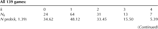
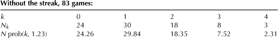
Looking at the first scenario we see that the Poisson assumption overestimates the number of no-hit games and underestimates the single-hit games, whereas when the streak is removed, in the second scenario, there is a very good fit to the actual data (rounding to the closest integer gives a nearly perfect fit). The poor fit to the Poisson distribution when the streak is taken into account means that in this instance the assumption that DiMaggio’s performance can be simulated by a coin-tossing experiment is unlikely. It was not for nothing that Stephen Jay Gould [57] was moved to call DiMaggio’s feat “The streak of streaks.”
A further affirmation that the data is from a Poisson process when the streak is removed is that whereas the mean λ = 1.23, the variance of the same data is 1.18. These values are very close, and, since another property of the Poisson process is that its mean and variance are the same, the closeness of these numbers lends support to the idea that hits are due to chance (consistent, of course, with DiMaggio’s skill, as determined by λ). This simply derived property of the Poisson distribution is used again in a telling manner in the subsequent section.
In case anyone wonders how the Poisson distribution fits the data within the 56-game streak, it is clear that there is a poor match simply because the probability of no hits is destined to be wrong; every game had a hit. In fact, in this case, in which λ = 1.63, the Poisson approximation gives results that are even worse than those in the first scenario. There are little grounds here for believing that the streak is due to pure luck.
This is not to say that an unusual streak cannot occur by chance alone, but the odds that this will happen is minuscule (about once in 10,000 seasons; there is a more detailed discussion of this in Section 6.7), and so the alternate hypothesis, that the streak is a sort of freak, is more in keeping with the Poisson model of random behavior. In the next section I show how the probability of getting a streak by chance alone is arrived at after we’ve had an opportunity to derive some formulas for runs, clumps, and streaks, however we may wish to call them.
It is worth pointing out that in each of three examples just given (bomb hits, fire alarms, and baseball hits), the probability p of a success never appeared, only the value of λ. To discuss these cases in terms of Bernoulli trials would require that the quarter-mile regions, or 15-minute intervals, or games in a season, would have to be further subdivided somewhat until at most one event can occur in the smaller sectors or intervals. This does not mean, however, that the value of p will always be very tiny, and the term “rare event” may, in these and many other concrete settings, be something of a misnomer. Let’s look at the case of baseball in more detail. Here the notion of Bernoulli trials taking place in time or space is replaced simply by a succession of epochs in which time is irrelevant. It is merely a concatenation of M trials, each trial being an opportunity to get a hit or not while at bat. How long it takes to conduct the trial is immaterial. The probability p of a success, namely, a hit, is estimated by the Law of Large Numbers as the average number of successes (the total number of hits T in a season for an individual player) divided by the number M of trials, namely, the batting average, BA. This number is typically between .2 and .4, not really very small.
In a temporal Poisson process, p is defined, roughly, for small time intervals h, as λh. What plays the role of h now is the reciprocal of the number of at-bat opportunities per game. To see this more clearly, note that λ = T/N = T/M × M/N = p × a constant. Therefore p = N/M × λ and h = N/M. Note, moreover, that the constant h depends solely on managerial decisions in the office and on the field (how many games to play this season and the number of times a player is given the opportunity to be at bat) and have virtually nothing to do with a player’s skill, and so BA and λ are proportional to each other, as one might expect.
Incidentally, since p is the probability of getting a hit, the probability of no hits in a game is (1 – p)b, where b is the average number of at-bats per game for an individual player (typically about four); therefore, the probability that he gets at least one hit in a game is 1 – (1 – p)b. But b = 1/h = N/M, as we just saw, so the probability of no hits per game is roughly (1 – λh)b = (1 – λ/b)b ∼ e–λ. How well does this last approximation match the probability of no hits per game, namely, e–λ, as obtained from the Poisson approximation? Let’s check it out. Consider DiMaggio’s 1,736 career games, for example. His lifetime batting average, with 2,214 hits, was p = .325, and λ was 1.28. Since there were 6,821 at-bats, we see that b = 6,821/1,736 = 3.93. In this case, (1 – λ/b)b = .21 while e–λ = .28, and there is agreement to one decimal place. It all seems to hang together.
I now want to extend the birthday problem considered earlier by generalizing it to the case of N people who share some significant event in common, not just birthdays, over a time period of c days (not just a year). There are C(N, 2) = N(N – 1)/2 ways of choosing pairs of people, and the probability that a pair share an event is 1/c, which gives the average number of shared occurrences as λ = N(N – 1)/2c. Therefore, the probability of no shared occurrence is, by the Poisson assumption,
![]() (6.12)
(6.12)
Before closing this section I return to the question of surprising coincidences by considering another lottery example, one that was mentioned at the beginning of this chapter.
In the February 28, 1986, edition of the New York Times it was reported that a woman from New Jersey won the weekly lottery twice in 4 months (“Odds-Defying Jersey Woman Hits Lottery Jackpot Second Time”). The first time it was Lotto 6/39 and the next time it was Lotto 6/42, meaning that each ticket is a random draw of six digits out of 39 or 42, as the case may be. It was declared that the probability of winning the jackpot twice in a lifetime is only one in 17.1 trillion, surely an unimaginable outcome for anyone, the New Jersey woman in particular.
Since the sample space for the first lottery consists of C(39, 6) equally likely possibilities and that for the second C(42, 6), then, assuming independence of the two draws, the probability of winning was computed as the product of 1 divided by C(39, 6) × C(42, 6), which is 10–13/1.71.
However, this computation is flawed since it assumes that both winning numbers were chosen in advance, whereas if we assume that the winner of the first jackpot purchased a single ticket, then the probability that the same person wins in the next lottery is simply 1/C(42, 6). Moreover, most people, this woman included, buy multiple tickets, say, five of them. In this case the probability p that the winner of the first lottery picks the winning number of the second lottery is then 5/C(42, 6) = 9.53 times 10–7.
Now consider 200 consecutive drawings (about 4 years of weekly drawings). We have here the ingredients of a Poisson approximation to 200 Bernoulli trials with probability p of a success. This means that λ = np = 200 × 5/C(42, 6), which is 1.98 × 10⁻⁴. Then the probability of any given player’s winning the jackpot two or more times is p0 = 1 – λe–λ – e–λ = 1.985 × 10⁻⁸. At this point it is reasonable to assume that about 10 million people play the lottery each week, giving rise, once again, to a Poisson approximation with 107 independent trials, each having probability of success p0. Then λ = 107 × 1.985 × 10–8 = .198. Therefore, the probability that at least one person in 10 million will, during the next 4 years, win the lottery at least twice is 1 – e–p0 = 1 – e–.985 = .727, which is not as preposterous as it originally appeared! This taming of a seemingly outrageous coincidence should serve to dispel the idea that all coincidences are mind-boggling events.
6.5 Not a Designer but a Gardener
Early in the twentieth century it was noticed that tiny percentages of certain strains of bacteria would continue to survive when an entire colony was placed in a toxic setting. Although it was generally understood that random mutations provide the raw material for natural selection among higher organisms, it was still controversial whether the ability of some bacteria to survive a hostile environment was due to the ability of a few to adapt to the killer virus or whether favorable random mutations that occurred all along prior to the toxic exposure is what allowed a few to survive. In a landmark paper published in 1943, biologists Salvador Luria and Max Delbrück [74] successfully carried out some experiments to resolve this question in favor of spontaneous mutations. In effect they vindicated the idea that even with microorganisms, evolution works “not as a designer but as a gardener,” an apt quote attributed to Jeff Bezos by Thomas Friedman (New York Times, May 19, 2012). The details of their investigation are given next. The key insight for interpreting their results is a very simple property of the Poisson distribution, namely, that the mean and variance are the same, which is why this is of interest to us.
More specifically, Luria and Delbrück grew a large culture of bacteria (E. coli B), cultivated in a flask from a single cell over many generations (doubling in population at each generation), and then exposed it to a bacteriophage (virus). The virus attacked the bacteria, and most were lysed. However, a few survived and gave rise to colonies that are resistant to the virus. What was not immediately obvious is whether the cells acquired their immunity by chance when the virus attacked, just as certain humans survive a massive epidemic of some deadly disease, or whether the immunity was there all along as a result of prior favorable mutations. In the first instance the survivors begin to produce resistant daughter cells that form small colonies that are then counted. Because there are billions of susceptible cells, this gives rise to a binomial distribution of immune cells just after they are impregnated with the harmful phage, which is why it can be approximated by a Poisson distribution.
On the other hand, if mutations occur spontaneously all the time, some cells become resistant before the virus is applied. The random mutations can happen in any of the previous generations; if they occur early on there will be many more resistant cells when the phage is introduced to the flask than if the mutation happened later, during the incubation of the bacterial culture. In this case, if the experiment is repeated many times, one obtains a roughly constant fraction of resistant colonies each time, since every cell initially had a rare but constant survival probability. Then each time the experiment is repeated, the variation in the number of surviving colonies from experiment to experiment will be much larger, since a mutation that took place early during the incubation will result in a large number of immune bacteria, all of them clones of the initial mutated cell, which will now have divided into many generations of daughter cells (clones are survivors of a single mutant ancestor).
Luria and Delbrück grew a large number of independent cultures from a single cell in separate flasks and then counted the number of mutant colonies just after being exposed to the virus. If mutations occur only on contact with the phage, the distribution of survivors from flask to flask should be roughly Poisson, as we said. However, if mutants occur haphazardly in each generation as the culture is growing, then the variance between flasks at the end would be much larger than the mean, and this is what they actually found. Think of each batch of cell culture as a separate baseball game in which there are 0, 1, 2, . . . number of hits. Similarly, the individual flask cultures will have 0, 1, 2, . . . surviving colonies of bacteria. In baseball, the mean is the number of hits per game over the season; for bacteria, this quantity is the number of surviving colonies among the total number of experimental batches.
In fact, from 20 separate flasks, 11 had no survivors; but in the others, the extant colonies ranged from 1 to 107 with a mean of 11.3 and a variance of 694, a far cry from what one expects from the Poisson distribution. To paraphrase the opening title (from a source that I can no longer recall), “Nature is an editor and not a composer.”
In Figure 6.1 we see both scenarios in action. The alternatives are between a mutation that is an adaptation to an induced challenge to survival and one that occurs spontaneously throughout the growth of the culture before being treated with the phage. This is represented by a hypothetical pyramid of four generations of a single cell, giving rise by doubling to 24 = 16 descendants, of which there are 8 mutants that belong to one clone in one instance, and we see the results of six flasks of culture. And the key to understanding this, as already mentioned, is the simple attribute of Poisson processes that their mean and variance are both equal, a fact that we used previously in discussing baseball streaks.

6.6 Chi-Squared
The ploy of dividing London into N small, bite-size sectors in order to discuss the bomb-hit data or total peak alarm times into 15-minute intervals or the 1941 baseball season into individual games was designed to exploit a test of statistical significance known as the chi-squared, or χ2, test. The test estimates the goodness of fit of a hypothetical distribution (the Poisson, in our case) to empirical data that has been arrayed into b bins corresponding to k = 1, 2, . . . , b events that occur per sector or interval, where c is the maximum number of occurrences. The squared difference between the hypothetical and actual estimates, summed over all bins, is taken as a measure of deviation and is called χ2. Small values of χ2 indicate a good fit and large values of χ2 a poor fit. Specifically,
![]() (6.13)
(6.13)
The crux of the matter is that Nk, with k ranging from 1 to b, is a sum of N Bernoulli variables Nk,j, defined by Nk,j = 1 if the jth sector has exactly k outcomes and is zero otherwise:
![]()
It follows that the sum of terms in (6.13) is, for large N, approximately distributed as a sum of normal random variables (this is the essence of the Central Limit Theorem, as discussed in Appendix A), and it can be approximated by the exact distribution for the sum of the squares of N normal variables having zero mean and unit variance known as the chi-squared distribution.
The b probabilities p(k, λ) are evidently constrained by the fact that they must sum to 1. Therefore, the independence of the b variables in the sum is reduced by 1. Moreover, λ is dependent on N, so there is a further reduction in independence, and we say that the χ2 test employs b – 2 degrees of freedom. The empirical distribution of χ2 in (6.13), namely, prob(χ2 < x), is a function F(x), which, for N large enough, can be approximated by the theoretical distribution FN(x) that random samples of χ2 are less than x. If one chooses x so that FN(x) = .95, as is customary, and if a specific sample χ02 has a value greater than x, we are inclined to reject the hypothesis that the data came from the specified distribution (Poisson, in our case), since 95% of all randomly chosen values of χ2 should be less than x. Otherwise, we (tentatively) accept the hypothesis.
Needless to say, after reading the previous chapter one might be tempted to raise a skeptical Bayesian eyebrow and be somewhat wary of this test, since it is, admittedly, an example of the kind of statistical modeling that was put in doubt there. It can be said, however, that the χ2 test is safe to apply in relatively benign examples in which the consequences of overstating the null hypothesis are really not so dire, as would be the case, say, in deciding on the efficacy of a drug that affects the health of patients. Its virtue is expediency, since it is relatively simple to apply, and it does provide a rough indicator of significance.
To be more specific, suppose that χ02 is the value of χ2 obtained from a particular set of data, such as found in the fire alarm example. Next, let p = 1 – FN(χ02) = prob(χ2 > χ02). If this probability is less than, say, .05, we tend to reject the null hypothesis that χ02 is a random sample from a Poisson distribution. We repeat that the exact distribution of χ2 as a sum of squares of normal variables having zero mean and unit variance is an approximation to the empirical χ2 statistic given by (6.13); a sketch of a proof of this can be found in Tijms’ book [109], pp. 416–419.
To recap the method: The empirical data of T sample data points is first broken down into N temporal or spatial segments, depending on the problem, within which there are either 0, or 1, or 2, . . . , or b occurrences and Nk is the number of segments having exactly k arrivals, for k = 0, 1, . . . , b, with ∑ Nk = N. Although the choice of N is somewhat arbitrary, the goal is to pick N so that each of the bins contains at least four or five entries. N can’t be too large; otherwise too many sectors will have zero or very few arrivals. By the same token, if N is too small, the segments contain too many points and it becomes difficult to test whether there are zero or just a few arrivals.
Typical values of χ02 for p = prob(χ2 > χ02) equal to .05 and .01 are obtained from the theoretical χ2 distribution, and we give these here:
| Degrees of freedom | p = .05 | p = .01 |
| 2 | 5.99 | 9.21 |
| 3 | 7.82 | 11.84 |
| 4 | 9.49 | 13.28 |
Thus, in the baseball examples, the data that includes streaks, there are 3 degrees of freedom, and the specific value of (4.4) has a value χ02 = 10.77 > 7.82, with a corresponding p-value of .0130, which is less than .05. Thus we reject the null hypothesis at this level. However, with the streak removed, χ02 = .24 and there is a p-value of .971, which is vastly beyond .05. In this instance we cannot reject the null hypothesis of a Poisson fit to the data. What this suggests is that the streak is an anomaly in which extraneous factors bias the number of hits through a combination of luck, skill, and determination. With the streak removed, the χ2 test is easily met, however.
In the fire alarm data there are 2 degrees of freedom and (6.13) takes on the computed value of .215. According to the χ2 test, 95% of comparable samples should have values not exceeding 5.92, so the Poisson hypothesis is accepted, with room to spare.
6.7 Stock Funds and Baseball Streaks, Redux
Many people are inclined to believe that a long binary string is random if it has more frequent alternations of zeros and ones than is actually the case, and a lengthy sequence of consecutive heads or tails or of any other binary variable is seen as due to something more than luck. The tendency is for individuals to reject patterns such as a long run as not typical of randomness and to compensate for this by judging frequent alternations between zeros and ones to be more typical of chance. Asked to produce a succession of digits to reveal a bias in favor of more alternations than an acceptably random string can be expected to have, people tend to regard a clumping of digits as a signature pattern of order when in fact the string is randomly generated. Confronted with HHHTTT and HTTHTH, which do you think is more random ? Both, of course, are equally likely outcomes of tossing a fair coin.
Psychologists Maya Bar-Hillel and Willem Wagenaar [8] comment that an individual’s assessment of randomness in tosses of a fair coin seems to be based on the
equiprobability of the two outcomes together with some irregularity in the order of their appearance; these are expected to be manifest not only in the long run, but even in relatively short segments—as short as six or seven. The flaws in people’s judgments of randomness in the large is the price of their insistence on its manifestation in the small.
The authors provide an amusing example of this when they quote Linus in the comic strip Peanuts. Linus is taking a true-false test and decides to foil the examiners by contriving a “random” order of TFFTFT; he then triumphantly exclaims, “If you’re smart enough you can pass a true or false test without being smart.” Evidently Linus understands that in order for a short sequence of six or seven T and F to be perceived as random, it would be wise not to generate it from Bernoulli trials with probability 1/2, since this could easily result in a nonrandom-looking string.
An illustration of how people misconstrue success runs in coin tossing is told by Theodore Hill [61]. On the first day of a probability course, Hill asks his students to record 200 flips of a fair coin, or, instead, they may choose to pretend to flip and then fake the results. The next day he amazes them by glancing at each of the student’s papers and reporting, in nearly all cases, which are true coin tosses from faked data. His ability to do so is based on the surprising fact that in a sequence of 200 tosses it is extremely likely that a run of six or more consecutive heads or tails will occur, as I show next. However, the typical person will rarely include runs of that length.
Let An(k) correspond to the number of sequences in which the longest run of heads doesn’t exceed k within a span of n tosses of a fair coin. Then, since the sample space consists of 2n equally likely strings of length n, the probability of the event Rn(k) that the longest run of heads doesn’t exceed k is
![]() (6.14)
(6.14)
The problem is to enumerate the favorable sequences An(k). I offer instead a simpler approach to runs, based on Berresford [19].
Define a run, clump, or streak of size k in a string of n coin tosses as a sequence of exactly k successive heads. We want to compute the probability P(n, k) of finding runs of size equal to or less than k. To do this we consider two mutually exclusive events:
i. There are runs of size equal to or less than k among the first n – 1 tosses.
ii. There are no runs of size equal to or less than k in the first n – 1 tosses, but the last k tosses out of n do form a clump.
Note that ii is the intersection of two independent events, the first being that the last k + 1 tosses are of the form tail followed by k heads (if these k + 1 tosses were all heads, there would be a run of size equal to or less than k among the first n – 1 tosses, which we exclude), and the second event is that there is no run within the first n – k – 1 tosses.
The probability of i is P(n – 1, k), whereas ii has the probability
![]()
Because i and ii are disjoint,
![]() (6.15)
(6.15)
To begin recursion (6.15), one has a couple of immediate identities: P(n, k) = 0 for all n < k, and P(k, k) = 1/2k, since a k-clump occurs in only one way in k tosses.
There is evidently a connection between (6.15) and the probability of An(i), defined by (6.14). In fact, since An(k – 1)/2n is the probability of no clumps of heads longer than k – 1, 1 – An(k – 1)/2n is the probability of having clumps of size k or greater in n tosses, and, as we just saw, this is the same as P(n, k). Thus,
![]() (6.16)
(6.16)
I have assumed that the probability of a success is ½. A slight variant of formula (6.15) for runs of size equal to or less than k in n tosses when the coin is biased, namely, when the probability p is not ½, is readily obtained using the same argument, and we get the following generalization:
![]() (6.17)
(6.17)
To put the formulas in to their simplest context I list here the 16 strings associated with n = 4:
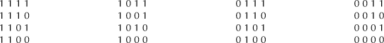
From (6.15) we find that P(4, 2) = .5 and P(4, 3) = .1875, and these values are immediately verifiable from the preceding table since there are eight runs of size equal to or less than 2, giving a probability of 8/16 = .5, and three runs of size equal to or less than 3, leading to a probability 3/16 = .1875.
Next, let’s compute P(200, 6) to get an answer to the question posed at the beginning of this section, the one in which Professor Hill asked his students to toss a coin 200 times. The likelihood that there is a clump of heads of size equal to or less than 6 is .8009, a better-than-80% chance. This unexpected result is what confounded Hill’s students.
Let me point out that the entire discussion could have been expressed in terms of binary strings generated by a Bernoulli process with p = 1/2, instead of coin tossing, asking for the probability of the longest run of either 0 or 1 in a string of length n.
Let’s conclude by asking about non-coin-tossing success runs. There are two examples of this kind that continue to invite controversy: streaks in sports and among fund managers.
I discussed baseball in Section 6.4 but left open, in the case of Joe DiMaggio, what the probability is of a streak of 56 consecutive games with at least one hit in a season of 139 games. His probability of getting at least one hit per game has been computed to be .81 during 1941, since his batting average that season was .346. Using (6.17), we find that the required probability of a streak is roughly 1 in 7,949, a minuscule chance. On the other hand, in the 83 games of that season that exclude the streak, DiMaggio’s probability of a hit in a game was .320, which leads for the case of at least one hit per game to a probability of .773 and for a 16-game streak to a probability of .244, a small but not improbable occurrence. As a matter of fact, DiMaggio did achieve a success run of 16 games in the 1941 season, and we see that this feat is not inconsistent with simple coin tossing.
In the financial world something similar seems to be at play. We told the story earlier of the well-known fund manager Bill Miller of the Legg Mason Fund, who, starting in 1991, was able to beat the S&P market index for 15 successive years. Assuming that he was just lucky and that his investment prowess was no better than tossing a fair coin each year, his probability of getting 15 successive heads is 1/215, or 1 in 32,768. However, allowing for a conservative estimate of 1,000 fund managers, each investing independently during that same period (there were actually about 6,000 managers as of 2008), the probability that at least one of them would attain such a streak by simple coin tossing now rises to about .03. To see this, we use a Poisson approximation to the binomial with λ = 1,000 × 1/32,768 and compute 1 – e–λ.
However, the odds for success are actually much better because active portfolio management has a history of more than 40 years. So the relevant question is the probability of attaining a streak of 15 heads (that is, beating the S&P) with a fair coin in 40 tosses among 1,000 individuals working independently. Using (6.15), this turns out to be .3377; if we use a more representative number of, say, 3,000 managers, this increases to .7094, nearly, 3 out of 4. To quote Leonard Mlodinow [84]: “I would say that if no one had achieved a streak like Miller’s, you could legitimately complain that all those highly paid managers were performing worse than they would have by blind chance.”
As it happens, Miller’s streak ended in 2005, and he has been subpar for several years since then, as we noted earlier. However, to criticize Miller is a bit disingenuous at this point because the same comment could have been made about DiMaggio; that is, if we take 3,000 ball players of his caliber and have them each play through the same 1941 season, the probability that at least one of them will have a 56-game streak is no longer negligible. Therefore, in fairness to Miller, one can argue, as we did earlier with DiMaggio, that his individual 15-year streak was an anomaly. Sure, it could have happened by chance, but the probability of this is so small that we discard this hypothesis in favor of saying that it was due to a combination of luck and skill and not just chance.
On the other hand, something that is not in Miller’s favor is that he, like most fund managers, begins his cycle of success with each new year. This is artificial, since cycles can start with any month within a year. It’s like saying that a hitting streak can begin only at the start of each new month. This makes the runs or streaks that start on the first of January even more special than they might be. Choose a different calendar year, and the streak could vanish. Miller himself acknowledges this in an interview in the January 6, 2005, Wall Street Journal, where he is quoted as saying “As for the so-called streak, that’s an accident of the calendar. If the year ended on different months it would be there and at some point the mathematics will hit us. We’ve been lucky. Well, maybe it’s not 100% luck—maybe 95% luck.”
6.8 Concluding Thoughts
“The ‘one chance in a million’ will undoubtedly occur, with no less and no more than its appropriate frequency, however surprised we may be that it should occur to us.” This quote is from R. A. Fisher, The Design of Experiments (Oliver & Boyd, London, 1937).
Physicist Richard Feynman is said to have opened one of his lectures with the following mischievous remark: “The most amazing thing happened to me today. As I pulled into the parking lot I saw that the car next to me had the license plate ARW 357. Isn’t that amazing? Of all the millions of plates in the state, what are the odds that I would park next to this car?”
Two good references to the psychology of coincidence are Falk [47] and Falk and Konold [46].
The mathematics of runs in coin tossing is also investigated, employing a somewhat different approach than the one used here, in two accessible papers, Bloom [21] and Schilling [102]. As applied to baseball, one should also consult Freiman [50].
A detailed account of DiMaggio’s game-by-game performance during his unbroken string of successes in the anno mirabilis 1941 can be found in Seidel [103]. It is of interest to compare the performance of Ted Williams in 1941. His batting average of .406 was higher than DiMaggio’s .357, though there was no comparable streak. Nevertheless, his unusual batting record does not match the expectations of a Poisson model, and, again, the assumption of random outcomes overestimates the no-hit games and underestimates the one-hit games. You may ask why Williams didn’t have a comparable streak. One possible answer is that, unlike DiMaggio, Williams walked to first base more frequently than DiMaggio, and, since these don’t count as hits, it means that a number of opportunities to continue a streak while at bat were squandered. Williams average of .406 has not been equaled since, a striking record in itself. Curiously, he also had a streak of 23 games that year, the longest of his career, that began on the same day as DiMaggio’s (see “Ted Williams .406 is More than just a Number” by Pennington, New York Times, September 17, 2011).
“Succinctly put, the Law of Truly Large Numbers states: With a large-enough sample, any outrageous thing is likely to happen.” This quote is from Diaconis and Mosteller [40].