7.1 Background

In this chapter I introduce a class of probability distributions known as power laws, because they have become modeling tools of considerable scope in a plethora of fields, the social and biological sciences among them, and because the literature regarding these distributions is scattered over many different books and journals representing myriad interests and is a little hard to pin down to one reference. A review of some of the salient features belongs in a book devoted to models in the social and biological sciences, as I hope to show, especially since the topic is surprisingly little known to people whose training in probability and statistics is based on the traditional core topics.

The core organizing principle in conventional probability theory is, as we saw in the preceding chapters (and will also see in Appendix A), the Central Limit Theorem, which tells us, roughly, that sums of independent random variables with a common mean and finite variances tend to a normal distribution. It is known, moreover, that random samples of certain variables, such as the heights of people in a given population, tend to drape themselves about the average value of a bell-shaped normal curve. The average represents a characteristic size for the population, and most individuals don’t deviate too far from that typical scale length. On the other hand there are numerous populations of variables that have no typical scale, since the variables range over a wide span and there is no characteristic value for their distribution. One thinks of the size of cities, which range from small towns of several thousand people to large metropolises whose populations are measured in millions (a number of other examples will be given later). In a sense to be made precise momentarily, being scale-free is an attribute of what is called a power law distribution, in which there are many small to medium-sized events interspersed with a smaller number of extreme happenings. The study of such scale-free distributions provides a statistical anchor for a large array of data that lacks a characteristic size and, as such, serves as an organizing principle that is similar, in some respects, to that of the normal curve in traditional theory. However, although conventional theory is set on a sound mathematical footing, it must be admitted that some of what is reported about power laws is speculative. Though there is certainly a solid core of mathematical validation, at least some of it is partly supported by heuristics that are not always convincing.

A number of mechanisms have been proposed for the existence of power laws, some of which I’ll review later. But essentially what seems to be at work here is that a large number of variables representing contingent events interact over a wide range of temporal and spatial scales. This manifests itself in a distribution of the frequency of sizes that possess what are generally called fat tails. This means that the occurrence of extreme events, though they are not frequent, is much more common than would be expected from the normal curve. As we will see, many natural processes follow such a distribution, as do manmade patterns such as the financial markets. In both instances catastrophic occurrences, such as large earthquakes and financial meltdowns (both of which were very much in the news as this was written) can be anticipated with more regularity than conventional probability models would lead one to believe. A concise summary of the difference between power law phenomena and events governed by the normal distribution is that the latter is descriptive of equilibrium systems, whereas the former deals with nature far from equilibrium, in a state of flux and turmoil. What the normal and non-normal laws have in common, however, is that they quantify levels of behavior in the aggregate, in which the erratic conduct of the individual is tamed when looked at as part of large groups of individuals. There is a certain amount of self-organization that emerges from the bustle of many interacting parts.

A function f(x) on the positive axis is said to be a power law if it is of the form

(7.1)

where b is a scalar that is usually between 1 and 3 and c is some other constant. In the discussion that follows, f is generally thought of as a probability density for some random variable X, which necessitates that there be some lower cutoff value in order to avoid unbounded behavior for small x. As a practical matter, this is not a serious restriction, since the data one actually deals with exhibits power law behavior only for sufficiently large x. In fact some authors say that f is a power law distribution if there is an asymptotic relationship

(7.2)

(meaning, as usual, that the ratio of the two sides tends to 1 as x gets larger). Under this interpretation the functional form of f for small x becomes less important, and, as we show later, f can be a bone fide probability density that exhibits power law behavior only when x is large. The use of a continuous density obscures the fact that the actual data sets that have been compiled are discrete and limited in range. It is more convenient, therefore, to consider the cumulative distribution function of X since it is defined for all x, and we may replace (7.2) by

(7.3)

Note that F(x), as 1 minus the integral of the density f from x to infinity, is also a power law, with an exponent b that differs by 1 from its value in (7.3).

Taking logarithms of (7.3) uncovers a linear relationship:

(7.4)

When plotted on a log-log scale, a power law appears as a straight line, at least for part of its range, and this is the key signature of such functions. In fact, in most of the examples profiled in the literature, the data is usually displayed in log-log form.

An important attribute of power law distributions is that they are scale-invariant, meaning that if one stretches or contracts the variable x by some factor s so that we now measure it on a different scale, then the shape of the density f(x) or, for that matter, the distribution F(x) remains unaltered except for an overall multiplicative constant that compensates for the fact that the data in the initial range is now stretched out or compressed:

(7.5)

where c(s) = 1/s^b. The interesting part of this story is that scale invariance implies a power law and therefore uniquely characterizes power law distributions by this scale-free property. To see this, assume that f is some function for which f(sx) = g(s)f(x) for any s > 0.

Take the derivative of f with respect to s and find that xf ′(bx) = g′(s)f(x). Now set b equal to 1 to obtain xf ′(x) = g′(1)f(x). This is a separable first-order differential equation whose solution is readily verified to be f(x) = f(1)/x^b, where b = f ′(1)/f(1).

One consequence of scaling is that the variability in some interval of length [x₁, x₂] is a constant multiple of the variability in the rescaled interval [sx₁, sx₂]. This is seen most readily (Figure 7.1) when b = 1, since, in this case,

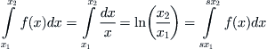
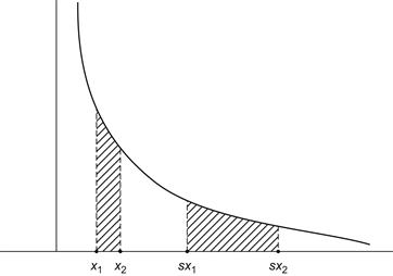
Thus, for example, there is just as much energy dissipated in many small earthquakes as in a few large seismic events, and the same can be said for the energy in wind turbulence, where there are a few large gusts interspersed among many smaller puffs. The sizes of moon craters is another instance, because there are small and large meteor impacts, and there are as many small species extinctions in the geologic record as large ones. I’m not making this up. These instances of self-similarity and many others in nature have been verified empirically. The most plausible explanation for this behavior is that the events we measure are due to a large ensemble of mechanisms, some large and others small, and it is the confluence of these many factors that results in a lack of prejudice with respect to scale. Individual occurrences are often multiplicative and contingent on each other, and the data spreads out considerably.

As mentioned earlier, some data displays a power law character over some wide range near the tail of the distribution and reverts to some other distribution for the remaining values. An example, to be discussed more fully in the next section, is the log-normal distribution, which is like the normal distribution for small x but with fatter tails when x gets large.

There is one more property of power laws that needs to be mentioned here: the lack of finite mean in certain cases. If the exponent b is less than 2, then the mean value of x can be computed from (7.1), assuming some lower cutoff value, and it is infinite. This follows because we accept the fiction here that the density f is continuous and the integration is out to infinity (see Section 7.4). For actual data sets, the mean is finite and can be computed, of course, and so the significance of an infinite mean is that as we accumulate more data the maximum of the data set increases and with it the mean. With larger and larger sets, the mean diverges. This is in sharp contrast to what happens with the normal curve.

For b > 2, the mean does settle down to a finite value, but now the variance becomes infinite unless b > 3 (see Section 7.4). Again, what this means is that as the data sets are progressively enlarged, the variances become unbounded.

7.2 The One-Percenters

The best way to understand power law distributions is to give some examples.

It has become commonplace in recent political rhetoric to refer to the superrich 1% of the population, because it appears unfair to some people that most of the wealth is in the hands of the very few, suggesting some kind of unhealthy imbalance in society. However, this phenomenon is not new and can be traced back more than a century. I begin with a plot of the fraction of people having income x in some large population. Vilfredo Pareto established in 1897 that the income distribution is, at least for the more affluent segment of the population, a power law with exponent b hovering in most cases about the value 2, more or less. What applies to income applies to wealth more generally or to the wages paid. If x_o is the minimum annual income, say, about $10⁴, then the percentage of people having an annual income at least 10 times that, namely, $10⁵, is

(7.6)

Thus, if b = 2, say, then only 0.1 of the population has an income of at least $100,000. When x equals 10 times that, a million dollars, then (7.6) gives 0.01, 1%; and for 10 times that, only a fraction, 0.001, one-tenth of a percent, have incomes exceeding that amount. Thus the fraction of people enjoying a certain level of income above the minimum is inversely proportional to the income level. To quote Mandelbrot and Taleb [77]: At its core, the power law of income illustrates the observation that “in a society, a very few people are outrageously rich, a small number are very rich, and the vast bulk of people are middling or poor.”

Interestingly enough, the well-known billionaire Warren Buffett, in an article in the New York Times (August 15, 2011) with the provocative title “Stop Coddling the Super-Rich,” offers a partial vindication of (7.6) by stating that in 2009 a total of 236,883 households in America had incomes of $1 million or more, and 8,274 households made $10 million or more. In this case a 10-fold increase in income translates into a roughly (1/30)-fold decrease in households, and, after a bit of juggling, we get an approximate b value in (7.6) of 2.47—not quite b = 2, but close. In another New York Times article, by Stuart Elliott (Sept. 12, 2010), we read that 59 million Americans (about 20% of the population) live in households having an annual income of $100,000 or more. Applying (7.6) again gives a b value of 1. 67, whereas 2% of the population live in households having annual incomes of $250,000 or more. This now provides a b value of 2.2—all in all, close to the Warren Buffett estimate and to the theoretical Pareto value of b = 2. Of course the last refers to household incomes in contrast to personal incomes, but we are in the same ballpark.

If we identify the fraction of people as the probability density that an individual has a given income x, then (7.6) asserts that

This can also be interpreted as the conditional probability of having an income greater than x, given that a person’s income is greater than x_o. In all candor, it needs to be said that for small-to-moderate values of x, Pareto’s data is best fit to a log-normal distribution. I’ll present more about this later.

An interesting consequence of these computations is what is called the 80-20 rule, as first observed by Pareto, who stated, as a variant to the income–wealth label, that 20% of the people (in Italy) held 80% of all the land.

The same observation applies to a wide array of instances; indeed, whenever there is a power law. Needless to say, 80-20 is just a convenient mnemonic for what in different settings might actually be 70-30 or 90-10 or even 99-1. But in all cases the top-heavy power function tells a story about levels of imbalance in society, a few more outrageous than others. Examples abound, though some may be anecdotal: 20% of the people generate 80% of the insurance claims; 20% of the workers in a firm do 80% of the work (an example that has been vouched for is that in which four people in a realty firm of 20 generate 85% of all sales); 20% of patients utilize 80% of the health care resources; 20% of a firm’s customers account for 80% of sales volume; 20% of all firms employ 80% of the workforce; and so forth.

An oft-quoted power law, due to George Zipf from 1949, is the distribution of the frequency of words in some text, such as Moby Dick. He prepared a ranking of words, from the most common, starting with the word the, followed by of, down to those least used. Then he plotted the frequency with which each word appears in the text and found that this is very nearly inversely proportional to its rank. To say that the rth most frequently used word has rank r is equivalent to asserting that r words have rank greater than or equal to r, and so the Zipf plot is actually a power law of the Pareto type, in which the fraction of words with rank equal to or greater than r is plotted against r.

Based on the 2000 census, we can plot the population of U.S. cities having more than a thousand people. Drawing a smooth curve through the data gives a density function as the fraction of cities whose population exceed x. This distribution is far from normal. Though one can compute an average size of U.S. cities, the individual sizes do not cluster about this mean value; there are many more small to medium-size cities than larger ones, and there is no tendency to cluster about this central value. We can apply the 80-20 rule to say that 20% of the cities harbor 80% of the U.S. population.

There are many other examples. In all cases the word fraction is interchangeable with percentage or frequency or, better, probability. Some of these are inventoried here and are described in more detail in some of the sources that can be found in the references. To acknowledge the origin of each power law separately would be to clutter the text, so I will do that for only select cases (see, however, Newman [90], Johnson [67], Montroll and Shlesinger [85], West and Shlesinger [116], and Browne [24]):

We could go on, but you get the idea. In all cases there are infrequent events having a large impact coupled with many events having little or no consequence.

One rationale for power laws, known as self-organized criticality, is often explained in terms of the sand-pile model. Here, grains of sand are dropped onto a flat surface until the sloping sides of the pile reach a certain critical incline beyond which any new grain begins to slip a little or a lot. At some point one falling grain results in an avalanche. It is the confluence of myriad small contingent events that produces an avalanche of any size, and it cannot be attributed to any single movement within the pile. Thereafter, when the tremor subsides, the pile starts to build up again until it reaches a critical state once more, and it is in this sense that it is self-organized.

The distribution of sizes is shown to be a power law, roughly 1/x. The disturbances caused by additional grains are contingent events, and it is argued by Per Bak [5] that the pile is a paradigm of many natural processes that organize themselves to a poised critical state at which minor disturbances can trigger a large avalanche. Earthquakes, forest fires, and species extinctions are all cited as examples of this. In each instance the footprint of a scaling law indicates a complex process organized to the brink of randomness simply as a result of the interactions among individual elements of the system. Many systems in nature that follow a power law hover between order and disorder, and every movement is the confluence of many effects, some small and others large, with no characteristic spatial or temporal scale, leading to changes for no discernible cause. They just happen. Significant external prodding can shake up a system and get it moving, but what occurs next is unanticipated.

It has even been suggested that the process of arbitrage in the financial markets may be self-organizing. The idea is that arbitrageurs tend to drive an economy to an efficient state where profits become very low and any negative fluctuation can cause an avalanche of losses that drive many arbitrageurs out of business. Thereafter they reenter the market and once again drive it toward efficiency. The power laws are then explained as fluctuations around the point of market efficiency. This is speculative of course (no pun intended), but it is a suggestive analogy nonetheless.

Physicist Per Bak [5] wrote a compelling book about self-organized criticality (referenced earlier) that is a paean to the ubiquity of power laws in nature. In an unfettered moment, he exclaims: “Self-organized criticality is a law of nature from which there is no dispensation.” This can be compared to the equally unbridled comment by Francis Galton, a century earlier, regarding the normal distribution: “I scarcely know of anything so apt to impress the imagination as the wonderful form of cosmic order expressed by the normal law; it reigns with serenity and complete self-effacement, amidst the wildest confusion. The larger the mob, and the greater the apparent anarchy, the more perfect is its sway. It is the supreme law of unreason.” Wow!

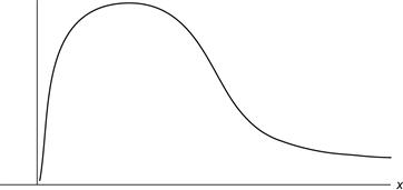
Here is a second explanation: A random variable X is said to have a log-normal distribution if log X is normally distributed. Here is one way it comes about. Begin with independent random variables having a common mean and finite variances, and, instead of adding them, multiply them together to obtain a variable X. Then the logarithm of X is the sum of the logarithms of the individual variables; therefore the Central Limit Theorem applies, and log X now tends to the normal distribution as the number of samples increases. This limiting distribution exhibits fatter tails than the normal distribution. For many processes, in fact, the log-normal is indistinguishable from a power law distribution for events that lie in the tail, especially when the random variable in question has a large variance (Figure 7.2). For more details, see Montroll and Shlesinger [85].

A specific process giving rise to the log-normal is the mechanism of proportional effect, meaning that over time an entity changes in proportion to its current size. The simplest version of this is a stepwise multiplicative process of the form x(t + 1) = a(t)x(t), with x(0) > 0, and a(t) are independent random variables. By iterating, one sees that

with the product taken over k from zero to t – 1. It follows that ln x(t) is a sum of independent random variables; assuming that their logarithms have finite variances, log x(t) will approach the normal distribution. This process offers somewhat of an explanation of the Pareto distribution of incomes, in which x(t) is the fraction of people, other than the superrich, with incomes t. Individuals with this income can acquire income t + 1 or have it reduced to t – 1 with a probability determined by the random variable a(t). As t increases, one reaches the log-normal as an equilibrium distribution.

The multiplicative effect is aptly characterized by Ben Franklin’s aphorism “For want of a nail the shoe was lost, for the want of the shoe the horse was lost, for the want of the horse the rider was lost.”

Finally, let’s discuss one last mechanism, perhaps the simplest of them all. Suppose, once again, that one has a growth process that is now exponential, defined by the function g(t) = e^at for some a > 0. The growth is terminated at random times determined by the exponential distribution e^–bt, with b > 0. Then the distribution of sizes is a power law. To establish this, observe that g(t) ≤ x if and only if t ≤ T, where x = e^aT. Therefore the probability that g(t) ≤ x is

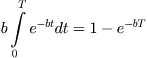
Inverting x = e^aT gives T = 1/a ln x, so the distribution function becomes F(x) = 1 – e^{–b/a ln x} = 1 – x^–b/a. By differentiating, one gets the density f(x) = (b/a)x^–b/(a–1), which is a power law for all x > 1. Since exponential interarrival times correspond to a Poisson process, one interpretation of the power law is that of an exponential growth process that is terminated at random times determined by a Poisson process. A number of compelling applications are given in Reed and Hughes [98].

7.3 Market Volatility

It should come as no surprise at this point that power laws and fat tails are also indicative of market volatility. Fluctuations in stock market prices and trading volume are just a couple of the variables that support power law distributions. In a provocative article in the Wall Street Journal, Mandelbrot and Nassim Taleb (author of a best seller [107]) state that the usual measures of risk in financial models are based on the normal curve, which disregards big market moves. “The Professors that live by the bell curve adopt it for mathematical convenience, not realism. . . . The numbers that result hover about the mediocre; big departures from the mean are so rare that their effect is negligible. This focus on averages works well with everyday physical variables such as height and weight, but not when it comes to finance.” They continue: “One percent of the U.S. population earns close to 90 times what the bottom 20% does, and half of the capitalization of the stock market (close to 10,000 companies) is in fewer than 100 corporations.” In other words, we live in a world of winner-take-all extreme concentration. We read that though conventional finance theory treats big market jumps as outliers that can be safely ignored when estimating risk, in fact just 10 trading days of big market jumps, up or down, can represent half the returns of a decade (Mandelbrot and Taleb [77] and Mandelbrot and Hudson [76]). The bottom line is: Expect the unexpected.

As we have seen, earthquakes are like this: lots of small quakes and the occasional large disruption. And so it is with the stock market. There are many players: Some are speculators that jump in and out of the market hundreds of times a day. Some are corporate treasurers and central bankers who trade only occasionally and at crucial moments. Others are long-term investors who buy and hold for long periods. They all come together at one moment of trading, and large fluctuations can result. According to Thurner et al. [108], the biggest influence may come from large funds that leverage their investments by borrowing from banks to purchase more assets than their wealth permits. During good times this leads to higher profits. As leverage increases, so does volatility, and price fluctuations display fat tails. When a fund exceeds its leverage, it partially repays its loan by selling some of its assets. Unfortunately, this sometimes happens to all funds simultaneously during a falling market, which exacerbates the downward movement. At the extreme, write the authors, this causes a crash; but the effect is seen at every scale, producing a power law of price disturbances. Recent events in the capital markets, such as the sudden Bear-Stearns near-collapse, testify to this, as did the plunge of 1987 and the crisis precipitated by Long Term Capital Management in 1998, to say nothing of the many meltdowns of 2008, 2009, and, most recently, 2011.

Interestingly, Bill Miller, fund manager at Legg Mason, who is celebrated for his 15-year streak of beating the S&P (we met Miller in Chapters 5 and 6, where this unusual streak is analyzed), is a supporter of the work of Farmer and Thurner. His comments in a CNBC interview on January 12, 2010, are worth repeating, from the perspective of a trader. When asked about the debacle of the past year, Miller stated, “The way the market operates, you know, we’ve got mean variance analysis and everyone knows they are the so-called fat tails, meaning that improbable events happen more than typically ought to in a normal distribution. But actually the market follows a power law distribution, which means that there tends to be—it’s like earthquakes, little corrections in the market, and then bigger earthquakes, recessions and then there’s a big one like the depression or a monster earthquake.” He goes on to say that now the danger has passed because the imbalances are in the process of being corrected, like tectonic plates readjusting after a quake (a large quake does not recur frequently), and therefore the risks are much lower now and it is a good time to invest again. It sounds like he is saying that, following a jolt, the system is free to self-organize to a new critical plateau, a new financial bubble. And that’s just what happened in 2011.

A not-too-dissimilar description of the dynamics of the marketplace can be found in The New Yorker, October 5, 2009, in which economist Hyun Shin says that during calm periods trading is orderly and participants can buy and sell in large quantities. When a crisis hits, however, the biggest players—investment banks, hedge funds—rush to reduce their exposure, buyers disappear, and liquidity dries up. When previously there were diverse views, now there is unanimity: Everyone is moving in lockstep. The process is self-enforcing. Once liquidity falls below a certain threshold, “all the elements that form a virtuous circle to promote stability now will conspire to undermine it.” The financial markets can become highly unstable. We have reached the same conclusion as before but in different words, and it is reminiscent of self-organized criticality.

Finally, I cite a peevish comment from another fund manager and advisor to the SEC, Rick Bookstaber. He complains on his website (Feb. 14, 2010) that the usual rant about business school quants misses the boat by thinking, all evidence to the contrary, that security returns can be modeled by a normal distribution. He sees this as a straw man argument. “Is there anyone on Wall Street who does not know that security returns are fat-tailed? Every year there is some market or other that has suffered a 10-standard-deviation move of the ‘where did that come from’ variety. I am firmly in the camp of those who understand that there are unanticipated risks.” He goes on to suggest that when an exogenous shock occurs in a highly leveraged market, the resulting forced selling leads to a cascading downward movement in prices. This then propagates to other markets, which now find that it is no longer possible to meet their liquidity needs. Thus there is a contagion based on who is under pressure and what else they are holding. Sound familiar?

7.4 A Few Mathematical Details

Suppose x₀ is the smallest value of the variable x and that f(x) = c/x^b. Then the average value of x is

which becomes infinite for b ≤ 2. For b > 2, the mean is finite, but a similar computation shows that the variance becomes infinite for b ≤ 3.

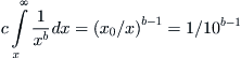
Note that the constant c can be obtained by imposing the condition

and, as before, this leads to the requirement that b > 1 if one is to avoid unbounded behavior at infinity. It is easy to verify that c = (b – 1)x₀^b–1 and, from this, that

(7.7)

In a similar manner one gets

(7.8)

However, if the density function is assumed to have an upper as well as a lower cutoff, which one can reasonably suppose when the actual data set that f approximates is indeed finite, then the case b = 1 is admissible.

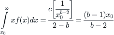
A more precise derivation of the 80-20 law is given here, at least for b greater than 2. If f(x) is the fraction of people in a given population having wealth x, then the integral of xf(x) from x to infinity is the total wealth in the hands of those people having a wealth greater than x; therefore the fraction of total wealth in the possession of those people is, using (7.7),

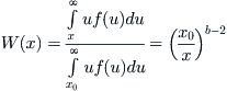
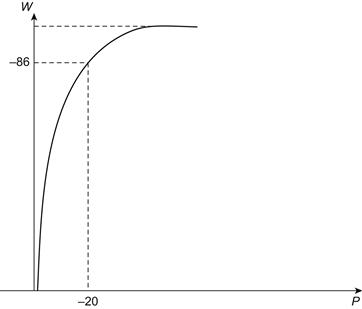
Next, using (7.8), we find that the fraction P(x) of people having wealth exceeding x is (x₀ /x)^b–1. Eliminating x₀/x from the expressions for W and P gives us

(7.9)

This relation can be plotted to give the curve shown in Figure 7.3, in which one sees that 20% of the people own more than 80% of the wealth (assuming that b is slightly bigger than 2).

7.5 Concluding Thoughts

Scale invariance is often associated with the idea of fractals, in which the statistical properties of a distribution appear the same at different levels of magnification. Thus, a coastline viewed from an airplane and as you stand at the edge of a rocky shore resemble each other in terms of the indentations and irregularities you observe, or, to cite another example, the veins in a leaf look like branches, and branches look like miniature trees. A specific example is the branching of a river basin; see Bak [5].