2.1 Background

Most public services are required to meet a weekly demand that varies over time in an uneven manner, often over all seven days of the week and 24 hours a day. The personnel available to match this demand profile must of necessity have overlapping shifts since no individual expects to work continuously over the week. This is unlike the private sector, in which work requirements are generally uniform, with a fixed “nine-to-five” workday that coincides exactly with the availability of personnel.

Examples involving public services are not hard to provide. It suffices to mention sanitation workers, police officers, ambulance drivers, nurses in a hospital, security guards, emergency work crews, airport baggage handlers, and transit workers, to name a few. In all these examples, the assignment of workers to different periods of the week is complicated by the fact that required workload does not match up to the available workforce.

In New York City, for example, there is effectively no refuse collection on Sunday (excluding certain private carting services). This means that there is even more garbage than usual waiting to be picked up on Monday morning because there is Saturday’s backlog to contend with in addition to the trash generated on Sunday. More sanitation workers are needed on Monday and—because some refuse, with its attendant smells and hazards, remains uncollected at the end of the day because of the overload—on Tuesday as well. One solution, of course, is to hire additional workers to fill the gap. However, in times of fiscal restraint this costly solution is unattractive to the municipality, which would prefer, instead, a restructuring of worker schedules to match the workload better. This requires some care, however. Any schedule that consists of irregular and inconvenient work shifts is unsatisfactory to labor. They prefer a regular pattern of workdays that gives the employee as many weekends off as possible, for example, or that meets some other “days off” requirement. There is a trade-off here between the needs of the municipality, which would like to get the job done in the face of severe fiscal deficits, and the labor union, which insists on a work schedule that is fair to its members (the questions of salary and benefits are separate issues that are ignored here).

In the next section, we discuss a mathematical framework for worker scheduling in the context of an actual labor dispute between the sanitation workers’ union and the city of New York that took place some years ago.

Let’s switch, temporarily, to what appears to be a different situation. The U.S. Constitution stipulates that “Representatives and direct taxes shall be apportioned among the several states which may be included in this Union, according to their respective numbers” (Article 1, Section 2). What this says, in effect, is that a fixed number of seats in Congress is to be allocated among the different states so that each state has representation in proportion to its population. This idea of one man–one vote is difficult to meet in practice because the division of seats by population is usually a fraction that must be rounded off. Because political power is rooted in representation, the rounding problem has been a source of controversy and debate throughout the history of the United States ever since Hamilton, Jefferson, and Adams first struggled to resolve this issue. They and their successors attempted to devise a method that would be fair to all states, meaning, among other things, that if a state gains in population after a new census count, then it should not give up a seat to any state that has lost population. We will examine this problem more closely in Section 2.3, where we see that what at first glance appears to be a reasonable solution can turn out to violate certain obvious criteria of fairness.

The apportionment problem should remind one of scheduling, in which a designated workload is to be shared by a fixed number of employees so that each worker gets a satisfactory arrangement of days off. Later, in Chapter 3, an analogous question arises in the context of deploying a fixed number of emergency vehicles, such as fire engines, to different sectors of the city so that they can respond effectively to calls for service in a way that is equitable in terms of the workload sustained by each fire company and that, at the same time, provides coverage that is fair to all citizens.

In a similar vein is the question of reapportionment, in which a given state with a fixed number of representatives to Congress must now decide how to divide up the state into political districts. There are a number of ways that a geographical area can be partitioned into sectors of roughly equal population, but partisan rivalry tends to encourage “gerrymandering,” in which irregularly shaped districts are formed to favor the election of one candidate over another. In this case, the allocation problem is compromised by considerations that are difficult to quantify.

There is an unexpected connection to the question of fair allocation of scarce resources to problems posed in the Talmud concerning the division of an estate among heirs whose claims exceed the available amount. Its most concise expression is framed by an ancient dispute and its resolution in the Talmud as “Two hold a garment; one claims it all, the other claims half. Then the one is awarded three-quarters, the other one-quarter.” Although the meaning of fairness is arguably different in this case, it bears a superficial resemblance to dividing any limited commodity, such as when urban districts need an assignment of fire companies or states vie for congressional seats, and the fire units or seats, as the case may be, are not available in the quantities desired. One requirement for fairness in the case of the Talmud will be that any settlement among a group of claimants continues to be applicable when it is restricted to any subset of contenders. This problem is discussed in Section 2.4, where it is related to a seemingly different problem regarding fraudulent financial schemes. The notorious Madoff scam of recent years, the largest Ponzi scheme ever, is still being contested as this is being written, since the amount owed to bilked investors exceeds by far the available funds from the defunct securities firm owned by Bernard Madoff. The scheme, incidentally, is named after Charles Ponzi, who carried out a similar scam in 1920 in Boston but on a smaller scale.

Evidently some of these questions are nearly intractable because they are too suffused with political harangue and backroom deals, while others are more susceptible to rational argument. The terms allocation, apportionment, assignment, deployment, or even districting and partitioning take on similar meanings, depending on the application, and when a nonpartisan mathematical approach can be sensibly used, it will often come in the form of an optimization problem with integer constraints. This is an approach that is common to a wide number of situations that are only superficially dissimilar, as we will see in this chapter and the next.

2.2 Manpower Scheduling

Before discussing the specific case of New York City sanitation workers, let us put the topic of scheduling workers in perspective by looking at another example first. Assume, as is the case in a number of public services, that each employee is assigned to five consecutive days of work followed by two days off. Moreover, if there are several shifts a day, a worker reports to the same time period, such as the 8:00 A.M. to 4:00 P.M. shift. This may not always be true (many urban police departments have rotating 8-hour shifts to cover a 24-hour day), but we limit ourselves to this simple situation because it already illustrates the basic ideas involved in scheduling.

Suppose that the total workforce is broken into N groups of very nearly equal size. In our case the only possibilities that exist for days off are Monday–Tuesday or Tuesday–Wednesday or . . . Sunday–Monday. Call these feasible periods “recreation schedules” and label them consecutively by the index j = 1, 2, . . . , 7. Suppose that it has already been determined that in order to meet the average demand, a total of n_i groups must be working on the ith day. That is, r_i = N – n_i groups are permitted off that day. Now let x_j be the number of groups that will be allowed to adopt the jth recreation schedule during any given week. For example, x₃ is the number of times that Wednesday–Thursday is chosen. We would like to develop a schedule so that each group has an identical pattern of days off during an N-week horizon, on a rotating basis. What this means will become more clear as we proceed.

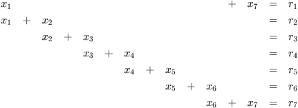
It is apparent that because Tuesday, for example, belongs to the first and second recreation schedules, then x₁ + x₂ must equal r₂. In general, the following system of constraining relations must be satisfied each week:

(2.1)

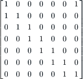
This system of equations may be expressed more compactly in matrix notation as Ax = r, where A is the matrix given by

Equations (2.1) are readily solvable by elimination. For example, if r₁ = 1, r₂ = r₅ = 2, r₃ = r₄ = 3, r₆ = 5, and r₇ = 6, the unique solution is x₁ = x₅ = 0, x₂ = x₄ = 2, x₃ = x₇ = 1, x₆ = 5. Thus the Tuesday–Wednesday schedule is followed twice, and so forth. Note that since each group gets exactly two days off a week, with N groups one must have

Therefore, by adding up Equations (2.1), it follows that

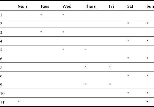
This means that we can construct a rotating schedule for each group over exactly N weeks. In the example just given, in which N = 11, an 11-week rotating schedule is exhibited in Table 2.1, where ^∗ denotes a day off. This chart can be read as either the arrangement of days off for any given group over an 11-week period (each row represents a week) or as a snapshot in any given week of the days in which the 11 different groups are off (each row is then one of the groups). When viewed as an 11-week schedule it is understood that in the twelfth week, the schedule repeats itself, starting again from the first row. Also observe that it is possible to permute the rows in any fashion. The particular arrangement of Table 2.1 is designed to avoid monotony for the workers by offering a variety of days off. The important factor is that on day i exactly n_i units are working, which is independent of row permutation.

It could happen that the r_i values are different in some other shift, say, 4:00 P.M. to midnight. In this case, a separate solution is obtained for this period using the same basic argument.

It would appear, therefore, that the matter has been brought to a close. However, there is a hitch. Although Equations (2.1) always possess a unique solution, it may not be an acceptable one. It is essential that the values of x_j be non-negative and integers, but this is not at all guaranteed. Consider, in fact, the situation in which all r_i = 1 except for r₅ = 2. Then x₃ turns out to have the value 1/2, as is easily verified.

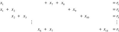
It appears that our choice of recreation schedules was too restrictive. To see this, let us augment the set of possible recreation schedules by allowing a single day off in a week. Index only Monday off, only Tuesday off, . . . , by j = 8, . . . , 14, and let x_j denote the number of groups that are permitted the jth recreation schedule, as before. Then because Monday, for example, appears on the first, seventh, and eighth recreation schedules, one must have

and, in general, system (2.1) is replaced by

(2.2)

It is now apparent that a non-negative integer solution to (2.2) always exists. It suffices to set x_i to zero for i = 1, 2, . . . , 7, and then let x_i+7 = r_i. Of course, this is an unsatisfactory solution for the workers who now have only one day off each week. A more acceptable solution would be one in which the number of six-day workweeks is as small as possible. This leads to the problem of minimizing the sum

(2.3)

or, equivalently, of maximizing

subject to constraints (2.2) and the condition that the x_j be non-negative integers. This is the first, but not the last, example we will encounter in this book of a type of optimization problem known as an integer program. Generally these problems are difficult to solve, but in the present case we can take advantage of the special structure of (2.2) to develop a simple algorithm that is suitable for hand computation. We sidestep the details (see, however, Section 2.5, Problem 1) since our main interest here is another scheduling question.

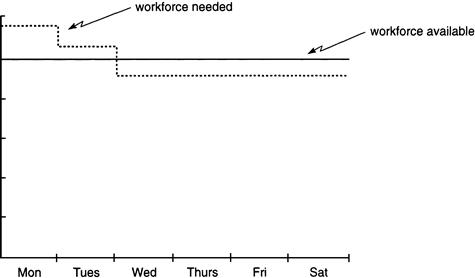
For many years the sanitation workers of New York City worked according to a six-week rotating schedule in which everyone got Sunday off and one-sixth of the workforce had off on Monday, another sixth on Tuesday, and so forth. This meant that, Sunday aside, only 5/6 of the workers were available on any given day. But, by the decade of the 1970s there was an escalating demand for refuse collection in the city, which translated into a requirement that actually 14/15 of the pickup crews should have been on the streets on Monday and 9/10 on Tuesday, clearly a mismatch between the supply of workers and the need for them (Figure 2.1). This discrepancy led the city to negotiate a new labor contract that would solve the problem without having to hire new workers. The story of how this came to pass is told elsewhere (see the references in Section 2.6), but for us the interesting part is how a revision of the work schedule would accomplish the goal.

A proposal was made to change the existing rotating schedule by dividing the workforce into 30 equal groups rather than 6. Recall that 14/15 of the sanitation crews are needed on Monday. This means that 28 out of the N = 30 groups should be working on that day, or, using our previous notation, n₁ = 28 and r₁ = N – n₁ = 2. The remaining days of the week have r values that had been determined to be r₂ = 3, r₃ = 4, r₄ = 7, r₅ = 7, r₆ = 7, and, of course, on Sunday r₇ = 30.

Guided by the need for integer solutions and mindful of the example worked out earlier in this section, we realize that the admissible recreation schedules will include six-day workweeks (only Sunday off) as well as two- and three-day weekends. Let x_i denote the number of times that a Sunday–Monday, Sunday–Tuesday, . . . , Sunday–Saturday schedule is chosen, i = 1, . . . , 6. A Friday–Saturday–Sunday three-day schedule is chosen x₇ times, while a Sunday–Monday–Tuesday combination occurs x₈ times. Finally, Sunday only is scheduled x₉ times.

Labor practices and union regulations stipulate that each worker is to get an average of two days off a week. With N = r₇ = 30, this means that

Because Monday appears on the first and eighth recreation schedules, it follows as before that x₁ + x₈ = r₁. Similar relations hold for the other days, and we therefore obtain

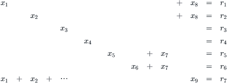(2.4)

Adding Equations (2.4) shows that

From the last row of (2.4) and the fact that r₇ = N = 30, we obtain

Taking the last two relations together gives

(2.5)

and, therefore, there are just as many six-day workweeks (only Sunday off) because there are weeks with three-day weekends off. At this point we pause to observe that, in the original six-week rotating schedule, a Saturday–Sunday–Monday combination would occur naturally every sixth week. The labor union would, of course, prefer to maintain this or some similarly advantageous weekend break under any revised schedule that might be proposed.

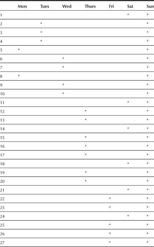
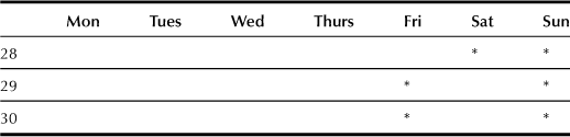
Let’s begin more modestly by asking for the schedule that gives the largest number of two-day weekends. That is, we want to maximize x₁ + x₆ or, equivalently, in view of relations (2.4), to maximize r₁ + r₆, – x₇ – x₈. The solution is quite apparent; namely, to let x₇ and x₈ be zero. This gives x_i = r_i for i = 1, 2, . . . , 6, with the remaining x_i all zero. The result is then a schedule that provides nine two-day weekends off every 30 weeks. Not bad! The rotating schedule itself is displayed in Table 2.2, which is to be read in the same way as Table 2.1. By suitably permuting the rows in Table 2.2 one can arrange to have five two-day and two three-day weekends, the schedule that was ultimately chosen in the labor negotiations for a new contract with the city of New York.

Returning now to the goal of having as many three-day weekends as possible, we see immediately from (2.5) that there is a price to pay for this luxury because it would require an equal number of compensatory six-day workweeks. This was not too attractive to the city since it meant that overtime pay had to be budgeted for the extra day. A compromise solution would have been to trade off two- and three-day weekends; indeed, after much discussion, such a compromise was selected.

A more formal approach to choosing a trade-off between two- and three-day weekends can be based on a decision to judge two-day weekends to be “worth” two-thirds of a three-day weekend. The goal, in this case, is to maximize the weighted sum

(2.6)

By relation (2.4) this is equivalent to maximizing

We can generalize from these examples to place the scheduling problem in a more abstract setting. Suppose there is a list of M feasible recreation schedules and that the jth schedule is chosen x_j times. Let a_i,j = 1 if the jth schedule contains day i, and set a_i,j = 0 otherwise. A is the matrix with entries a_i,j, and we require that Ax = r, where r is a vector with components r_i, the given number of groups that can be allowed off on day i, and x is the vector with components x_j. The problem is to choose the non-negative integers x_j so as to maximize a weighted sum

in which c_j are given non-negative quantities. The two cases considered previously are instances of this integer programming formulation.

2.3 Apportionment

Throughout its rich history the number of states in our country has increased from the original 13 to the present 50, so at any moment there were N states, with populations p₁, p₂, . . . , p_N. The number of seats in the House of Representatives also grew from an original 65, and at a given moment in history it had a value of h, with h never less than N. The seats are apportioned among the states, with a_i allocated to state i. The sum of the a_i equals h; of course, the a_i must be integers, with at least one per state. The exact share of h to which the i state is entitled, its quota q_i, is simply the fraction of h that is proportional to the population of that state, namely,

We have already mentioned the dilemma faced by Congress in allotting these quotas: They need not be integers!

A number of schemes have been devised over the years to mitigate this difficulty. First note that if some q_i is less than 1, then it must be set to unity. Because the House size remains at h, the remaining q_i must be adjusted accordingly. This leads us to define a fair share s_i as the largest of the numbers 1 and cq_i, where c is chosen so that the sum of the s_i is now h. For example, if h = 10 and N = 4, with populations of 580, 268, 102, and 50 (thousand), then the quotas q_i are 5.80, 2.68, 1.02, and 0.5. The last state is entitled to one seat, and the remaining nine seats are apportioned among the remaining three states, whose quotas are now 5.49, 2.54, and 0.97. Again, the last state is given exactly one seat, leaving eight to distribute among the other two, whose revised quotas are 5.47 and 2.53. Therefore s₁ = 5.47, s₂ = 2.53, s₃ = s₄ = 1. In 1792 Alexander Hamilton proposed to give the i state the integer part of s_i, denoted by [s_i], and to allocate the remaining

seats, one each, to the states having the largest remainders. From a mathematical point of view, this amounts to choosing integers a_i ≥ 1 so as to minimize the sum

(2.7)

subject to the condition that

(2.8)

which, once again, is an integer programming problem. In effect it asks for integer allocations a₂ that are never less than unity and are as close as possible to the fair shares s_i (which need not be integers), in the sense that they minimize the squared difference (2.7) while observing constraint (2.8). This problem admits a simple solution that is identical, as we will see, to Hamilton’s proposal. Begin by assigning one seat, the least possible, to each state. Clearly 1 = a_i ≤ s_i. Next, add one more seat to the state i, for which the difference

(2.9)

is largest. The key idea here is that a_i appears only in the ith term of the sum (2.7), and so (2.7) is made smallest by allocating the additional unit to the term that most decreases the sum. Continuing in this fashion we eventually must assign a_i = [s_i] seats to each state. The reason for this is that, as long as a_i + 1 < s_i, adding another unit to state i can only contribute to the reduction of (2.7), and this remains true until a_i is equal to [s_i]. Thereafter the remaining k seats are distributed, one each at most, to those states for which, by virtue of (2.9), the remainder s_i – [s_i] is largest.

Hamilton’s idea is, at first sight, a reasonable one, and so it was adopted for a time during the nineteenth century. Eventually, however, it was shown to be flawed. This happened after the 1880 census, when the House size increased from 299 to 300. The state of Alabama had a quota of 7.646 at 299 seats and 7.671 at 300 seats, whereas Texas and Illinois increased their quotas from 9.640 and 18.640 to 9.682 and 18.702, respectively. Alabama had previously been given 8 seats of the original 299, but an application of Hamilton’s method to h = 300 gave Texas and Illinois each an additional representative. Because only one new seat was added, this meant that Alabama was forced to give up one representative, for a new total of 7. This paradoxical situation occurred in other cases as well, and it resulted, ultimately, in scrapping Hamilton’s idea. What was being violated here is the notion of House monotonicity, which stipulates that, in a fair apportionment, no state should lose a representative if the House size increases.

Thomas Jefferson had a different idea in 1792. He recommended that a_i be the largest of 1 and [p_i/x], where x is a positive number chosen so that the sum of the a_i equals h. As before, [.] means “the greatest integer part of.” The role of x is to be a unique divisor of the population p_i of each state so that representation is determined by the quotient P_i/x. If one state has a greater population than another, its share of House seats is no less than that of the smaller state.

Jefferson’s method can be formulated differently. Let S be the subset of all states for which a_i > 1. Then, for each i in S,

where 0 ≤ y_i < 1 is a number that is zero when p_i/x is an integer. By cross-multiplying it follows that

That is, x does not exceed the minimum of p_i/a_i over all i in S. From the left side of the inequality we obtain x > p_i/(a_i + 1). When [p_i/x] ≤ 1, then a_i = 1 and so p_i/x < a_i + 1. In all cases, then, x is greater than the largest of p_i/(a_i + 1). Putting all this together gives

(2.10)

where min and max are shorthand, respectively, for “minimum of” and “maximum of.”

Conversely, if (2.10) is satisfied, then the right side of the inequality shows that 1 ≤ a_i ≤ p_i/x for each i in S, while the left side of (2.10) gives us a_i + 1 > p_i/x for all i. Therefore a_i = [p_i/x] for all i in S; otherwise a_i + 1 ≤ p_i/x, which is a contradiction.

However, when Jefferson’s method was applied to the 1792 census, in which h = 105, an anomaly occurred in which Virginia’s fair share of 18.310 was rewarded with 19 seats, whereas Delaware’s share of 1.613 gave it only one seat. The larger state was favored over the smaller one, an imbalance that was frequently observed using Jefferson’s method from 1792 to 1840, during which there were five censuses. John Quincy Adams proposed a modification of the procedure in which [.] now means “rounding up” to the next largest integer. But this tended to favor smaller states at the expense of the larger ones. Daniel Webster suggested a compromise in 1832 in which [.] was to mean that one rounds off to the nearest integer. By an argument similar to the one given earlier, Webster’s method implies the existence of an x for which

(2.11)

and it seemed to give results more reasonable than either of the methods proposed by Jefferson or Adams. Indeed, as Balinski and Young argue in their thorough discussion of the problem (their book is referenced in Section 2.6), Webster’s method goes a long way toward satisfying a bunch of fairness criteria, including the previously mentioned House monotonicity requirement. Interestingly, Webster’s approach, which was adopted for only a decade beginning in 1840, also satisfies an integer program. To show this we observe first that the per capita representation of state i is a_i/p_i, whereas the ideal per capita representation, across all states of the Union, is h/p, where p is the combined population of all states together. Consider now the sum of the squared differences of a_i/p_i to h/p, weighted by the population of state i:

(2.12)

Choosing integers a_i ≥ 1 to minimize (2.12), subject, of course, to their sum being equal to h, we get Webster’s method. In fact, since h²/p is constant, we see from (2.12) that it suffices to minimize the sum of the a_i²/p_i. If an optimal choice has been made, then interchanging a single seat between two states r and s cannot reduce (2.12) when a_r > 1. Keeping the allocations to all other states the same, the interchange implies that

or

(2.13)

We claim that

for otherwise there exist integers r and s for which (2.13) is violated. Condition (2.11) is therefore satisfied.

Although mathematical convenience often dictates the choice of an objective function in a minimization problem, the previous examples should dispel the idea that this can be done with impunity. The decision of what function to optimize must be examined carefully in terms of the intended application. Another example of this ambiguity will appear in the next chapter.

We close by touching on the reapportionment problem mentioned at the beginning of this chapter, in which a state with k representatives must now partition its geographical area into political districts. Even more than the apportionment issue, the question of districting is rooted in a struggle for power, since it affects directly the ability of a candidate to be elected to Congress. The ethnic and racial makeup of a neighborhood can favor one political party over another, and the way district boundaries are drawn affects the balance of votes. Nevertheless, one can at least pose some aspect of the problem mathematically, and, even if it is somewhat artificial, the formulation is useful in terms of applications to more benign problems of partitioning a region into service areas, such as school districts, postal zones, or police precincts.

Suppose that the state is divided into N parcels of land, census tracts to be specific, and that we wish to form k contiguous districts from these parcels to correspond to k seats in the House of Representatives. Imagine, by looking at a map of the state, that a number M of clusters of the N parcels has been formed, generally overlapping, that constitute potential political districts. The procedure for actually carrying out this partitioning is a separate matter that can itself be formalized, but we bypass this step here, much as we skipped the question of how feasible “recreation schedules” were formed in the manpower scheduling problem. The only requirement in forming the M clusters is that they be feasible in terms of being reasonably compact in size and not too misshapen (not too “gerrymandered”) as well as connected (no enclaves).

Let a_i,j = 1 if tract i belongs to the jth feasible cluster, and let a_i,j > 0 otherwise; and let x_j = 1 if the jth cluster is actually to be chosen as one of the political districts, with x_j = 0 otherwise. The population of tract i is p_i and so the total population of cluster j is

If p is the state’s total population, then the population of each district should ideally be p/k to achieve equal representation. In effect, p(j) should differ from p/k as little as possible. This leads to the integer program of minimizing the sum of squared differences

subject to the constraint

which ensures that exactly k districts are formed out of the M potential ones. Whether this formulation has any merit in practice is arguable but at least it poses the problem in a coherent and parsimonious manner and helps us to recognize the possible connections to similar districting problems.

2.4 An Inheritance in the Talmud and Madoff’s Scheme

The Babylonian Talmud of nearly two millennia ago records religious and legal decisions of that time. The Talmud includes the Mishnah, or rulings, followed by rabbinical commentaries on the Mishnah. One fascinating problem recorded there tells of three heirs who lay claim to an inheritance of 100, 200, and 300 units (which, for simplicity, we think of as dollars). However, the estate is worth less than the sum claimed by the heirs. For an estate of 100, 200, and 300 dollars, the Mishnah arbitrates the claims as shown in Table 2.3.

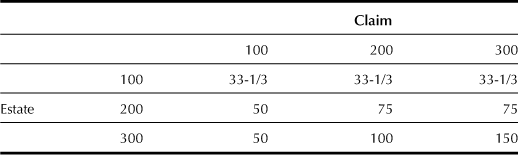
This is a puzzling division. When the estate is small it is divided equally among the heirs, but as the estate grows it is divided either proportionally or in some manner that seemingly bears no relation to the other divisions. What could they have been thinking? Is this a fair division?

To understand the rationale behind the allocations, let’s quote another, more straightforward Mishnah that reads “two men hold a garment; one claims it all, the other claims half. The one is awarded 3/4, the other 1/4.” The principle here seems simple enough. One claims half the garment and so concedes the remaining half to the other. What continues to be in dispute is the remaining half, and this is divided equally. By implication, if both claimed the full garment, it would be divided equally between them, each getting half.

A more general version of the heir’s problem is for n heirs or creditors, as the case may be, having claims in the amounts of d₁ ≤ d₂ ≤ … ≤ d_n, with D = ∑ d_i ≥ E, where E is the size of the estate or debt. The goal is to find a corresponding division of E so that the creditors receive shares x₁ ≤ x₂ ≤ … ≤ x_n in which E = ∑ x_i. This satisfies at least one fairness criterion, in that a larger claimant never receives a smaller amount than a lesser claimant; that is, x_i ≤ x_j when d_i ≤ d_j.

Let’s begin with a more careful analysis of the contested-garment problem. Let u₊ denote the larger of u and zero. If person i imposes a lien of d_i, then the uncontested amount is E – (E – d₁)₊ – (E – d₂)₊, and this, as with the garment, is divided equally. In addition, person i concedes an amount (E – d_i)₊ to person j. Thus

(2.14)

for i, j = 1, 2 and i ≠ j.

It is useful to restate (2.14) in the following manner to show how it depends on E. When E is less than or equal to d₁, the estate is divided equally; but as soon as E exceeds d₁, the lesser creditor receives half of his or her share and then temporarily drops out while the larger claimant continues to gain an amount E – d₁/2 until E has reached the value of D/2. At this juncture x₂ = d₂/2, and each creditor has now achieved half his or her respective claims. As E continues to increase, they again divide the additional amount equally until the first creditor receives his full share of x₁ = d₁ and departs. The balance then all goes to the higher claimant until, finally, E reaches a value of D. At this point, x₂ = d₂, and both creditors are vindicated.

Note that (2.14) is increasing monotonely with E, so no creditor receives less than before if E happens to increase.

To extend the two-person allocation to n people, another fairness criterion is invoked, which stipulates that the division is internally consistent. What this means is that the amount allocated to any subset of claimants is the same allocation they would have gotten as part of the larger group. Put another way, if S is any subset of the creditors, then the share E_s that they receive as a group from the arbitration is itself divided among themselves according to the same rule. The number of individual shares they each get from E_s is the same as the numbers awarded under the rule applied to the entire group of n people. In particular, if S consists of two individuals i and j, and if they receive a total between them of x_i + x_j from the arbitration of n people, then the amount E_s = x_i + x_j is allocated so that i gets x_i and j gets x_j. It is left as to Problem 4 of Section 2.5 to show that a consistent arbitration rule is determined uniquely.

For simplicity we limit the following discussion to the case of three people, but a similar reasoning applies in general. A rule is proposed that is consistent with the contested-garment principle when applied to a subset of two individuals.

If E is less than or equal to d₁, the total amount available is demanded by each claimant, and so it is divided equally. However, as soon as E exceeds d₁, the two-person contested garment rule is applied with person 1 versus a coalition of persons 2 and 3. Thus x₁ is d₁/2, and the remainder is divided between 2 and 3, again according to the garment rule. This means that if E is less than or equal to d₂, the remaining amount, (E – d₁/2)/2, is divided equally between these two individuals, whereas if E exceeds d₂, then x₂ equals d₂/2 and x₃ = E – (d₁ + d₂)/2. When E reaches D/2, it is easy to see that x₃ becomes d₃/2, and each contestant has achieved half his or her due. As E continues to increase, the additional amount is divided equally until the lowest claimant drops out, having attained d₁. The same rule applies to the other two individuals until the one attains d₂, and the remainder goes to the highest claimant who finally achieves d₃ when E has the value D.

Applying this rule to Table 2.3 shows that an estate of 100 is divided equally, whereas an estate of 200 ensures that the lowest claimant obtains half his lien, namely, 50, with the remainder split equally among the others, namely, 75 each. Finally, when E is 300, both the first and second claimants get half their due, 50 and 100, respectively, with the remaining 150 going to the largest claimant. Thus, what at first appeared to be a capricious subdivision of the estate now seems natural in retrospect. An inspection of Table 2.3 also reveals that the divisions satisfy the consistency requirement.

The arbitration rule undergoes a subtle shift in interpretation as E passes D/2. For E below that level, one thinks of the x_i as awards but beyond D/2 the focus is on the loss d_i – x_i that is incurred. This finds a resonant echo in the Talmudic script where one finds, in essence, that “less than half is nothing, more than half is all.” In effect, getting half the lien is worthless and can be written off, so any award is found money. However, getting more than half is frustrating, since one begins to hope of achieving full restitution and anything less than that is a deprivation. This is a version of the glass-half-empty or half-full cliché.

When the inheritance rule is applied to congressional apportionment it meets some of the criteria of fair apportionment, in the sense that any apportionment acceptable to all states remains acceptable to any subset of states being considered. Hamilton’s apportionment scheme, discussed in Section 2.3, violated this criterion, although it was met by the proposals of Jefferson and Webster. An example of this lack of uniformity is illustrated by the case of Oklahoma, which became a state in 1907. Up to that time, the House consisted of 386 seats, apportioned, according to Hamilton’s method, so that New York had 38 members and Maine 3. Oklahoma’s entry entitled it to 5 seats, which it received, and the new House size was 391. However, under Hamilton’s method, New York would now be forced to give up 1 seat in favor of Maine, for a total of 37 in New York and 4 in Maine, even though the population in each state had not changed.

Late in 2007 an enormous financial scam was revealed, a so-called Ponzi scheme, that was orchestrated by financier Bernard Madoff. The way this worked is that early investors were given high returns that were paid from money reaped from later investors. More and more people needed to be lured into the scheme to feed the fraudulent upside pyramid of wealth until it finally collapsed for lack of a sufficient harvest of fresh funds. The amount owed to his numerous creditors reached into the billions of dollars, but the total value of his remaining estate, including yachts and seaside villas, was only in the millions. The trustee assigned to resolve the multiple claims had the formidable task of sifting through the various demands for restitution and legal challenges, some more pressing than others, and the question of an equitable distribution of assets now loomed. Though it would be too much to believe that a solution similar to that imposed in the Talmud would be workable here, it is clear that some kind of fair retribution could be carried out that observed some of the same principles. Several claimants had their life savings wiped out, while other lost more modest amounts. It has been suggested that the former group should have priority in any settlement. In fact, if actual dollar loss is replaced by percentage loss relative to a victim’s total wealth, then a person of modest means who is wiped out would now have a larger claim than a wealthy person who lost only part of her estate, even though the total dollar loss in the latter case is much larger than for the former. At this writing the lengthy process of satisfying Madoff’s many victims—nearly 9,000 of them at the latest count—continues unabated.

An interesting twist to this story is that the trustee in charge of getting money back for the net losers planned to “claw back” money from the net winners, who took out more than they put in. After all, some of the early investors actually profited from the scheme. The courts have decided not to wade into this matter, which is further complicated by the fact that many of the larger financial institutions that gained from their involvement with Madoff are exonerated from the “claw back” because their executives, to quote an article in the New York Times, “declined to look too deeply into Madoff—even though internally they had acknowledged that his returns were too good to be true.” What saves them is a legal principle of pari delicto, that is, “a thief cannot sue a thief” since the trustee is acting on behalf of Madoff, a thief, and so by alleging that the large banks played a conspiratorial role in the fraud, he is granting them a legal disclaimer.

2.5 A Few Mathematical Details

In order not to disrupt the presentation in the previous sections with too many details, I deferred two mathematical asides to here.

An algorithm for minimizing (2.3), subject to constraining relations (2.2), is not hard to implement. From (2.2) we observe that

in which x₀ is set equal to x₇ and j = 1, 2, . . . , 7. The same relations also show that

for all j. Now define

(2.15)

in which r₈ is set equal to r₁. The last equation in (2.2) shows that

(2.16)

and so it follows that x_j are non-negative for all j. The algorithm begins by choosing an initial value of x₀, namely, x₇, in relation (2.15), to compute x₁. From (2.16) we see that there is only a finite number of choices. Since x_j takes on the largest possible value for each j = 1, 2, . . . , 7, it suffices to apply (2.15) for each initial choice of x₀ and to compute the corresponding sum of the x_j to obtain the largest possible sum. The same choice also minimizes (2.3) because (2.15) always picks the value r_j – x_j−1 (unless constrained to choose the smaller value, x_j+1) and this then forces x_j+7 to be zero. Otherwise x_j+1 is non-negative (show this!).

Try this procedure for the case in which r₁ = 5, r₂ = r₅ = 2, r₃ = 6, r₄ = r₆ = 3, and r₇ = 1. We see that x₀ is either zero or 1, and so there are two possible solutions to the integer program.

In Section 2.4 we left unproven the internal consistency of the allocation scheme. I do that now. Suppose that an estate E has two allocations x₁ ≤ x₂ ≤ x₃ and y₁ ≤ y₂ ≤ y₃ and that x_i < y_i for some i. If x_j ≤ y_j for all j ≠ i, then E = x₁ + x₂ + x₃ < y₁ + y₂ + y₃ = E, which is impossible. Therefore, x_j > y_i and x_i ≤ y_i, for some j ≠ i (^∗).

Let S be a subset of contestants containing only i and j. Then S gets an allocation of E_S equal to either x_i + x_j or y_i + y_j. Suppose that x_i + x_j ≤ y_i + y_j. Internal consistency means that under the allocation x_i + x_j the ith contestant gets x_i and the jth gets x_j, whereas under an allocation of y_i + y_j the ith person gets y_i and the jth receives y_j. Because of monotonicity, y_j must not be less than x_j, which contradicts (^∗). A similar argument shows that (^∗) is again contradicted whenever y_i + y_j < x_i + x_j. It follows that x_i = y_i for all i.

Finally, there is an interesting comment on the question of internal consistency. Suppose that N customers share a public facility such as a reservoir. The cost of the service must be allocated fairly among the users by a system of fees. This is a topic that is not unrelated to the apportionment problem, and it has a number of ramifications. We touch on only one aspect here.

Let S be a subset of the N users and C(S) be the least cost of servicing all the customers in S most efficiently. If S is empty, then the cost is zero. Moreover, if x_i is the fee charged to the ith customer, we impose the breakeven requirement that

Because the N customers are cooperating in the venture of maintaining the utility, it seems reasonable that no participant or group of participants should be charged more than the cost required to provide the service:

(2.17)

A related idea is that no participant or subset of participants should be charged less than the incremental cost of including them in the service. Since the incremental cost is C(N) – C(N – S), we require that

(2.18)

Inequality (2.17) expresses the incentive for voluntary cooperation among the participants, whereas (2.18) is a statement of equity, since a violation of this inequality by some subset S of users means that S is being subsidized by the remaining N – S customers. In effect, these inequalities express the idea that the individuals have formed a coalition to share both costs and benefits fairly. It is not hard to show that (2.17) and (2.18) are equivalent.

2.6 Concluding Thoughts

The revised New York City sanitation work schedules were agreed on in a new contract in 1971 and, according to the New York Times (“City wants to redeploy sanitation men for efficiency,” February 11, 1971, and “Sanitation union wins $1,710 raise in 27-month pact,” November 17, 1971), “city officials described the new pact as a major breakthrough in labor relations in the city because salary increases were linked to specific provisions to increase productivity.” The complete story is told in the Mechling paper [81]. A review of the mathematics of manpower scheduling is by Bodin [23].

The apportionment problem for the U.S. Congress is captivatingly discussed in the book by Balinski and Young [7]. One of the pitfalls of modeling optimization questions was revealed in Section 2.3, in which we saw that a formal minimum provided little or no guidance in resolving the underlying issue of fairness.

The reapportionment, or political districting, problem is illustrated by the troubled experience of California, which had gained 7 new seats in the preceding census to give it a total delegation of 52 members to Congress in 1992 (“California is torn by political wars over 7 new seats,” New York Times, March 3, 1991). There is a similar example from New York (“U.S. court voids N.Y. congressional district drawn for Hispanic,” New York Times, February 27, 1997).

The inheritance problem from the Talmud is thoroughly treated by Aumann and Maschler in [4] and by O’Neill in [92]. The Madoff scheme gets a comprehensive review in two New York Times articles by Enriques [44] and Nocera [91]. A good overview of this and other issues raised in this chapter can be found in a paper by Balinski [6].