
While the City Burns
3.1 Background
What began as a flare-up on the kitchen stove quickly spreads to the wooden counter, and smoke fills the room. An alert homeowner calls the emergency fire department number, and within minutes a fire engine company, siren blaring, shrieks to a halt in front of the apartment, and the blaze is shortly under control. Scenes like this are enacted daily in cities and towns all over the country and are familiar enough. But sometimes the consequences are more dire, and there could be considerable loss of life and property. To reduce these losses, if not to eliminate them entirely, is the primary mission of a fire department whose size and operation must be adequate to match the level of service required of it by the public. Insurance codes and municipal regulations stipulate a minimum of coverage, to be sure. But during periods of escalating demand, especially in inner-city ghettos, the number of incidents stretch the available resources. City budget cutbacks and fiscal belt tightening make it less probable that more firefighting equipment and personnel can be added to the existing departmental roster, which forces the chief and his or her aides to rethink the deployment of the forces currently at their disposal to make them more effective. Although we focus here on fire services, the same predicament faces virtually all public emergency services, including ambulance, police, and repairs.
The number of fire companies and their geographic distribution affect the ability to respond to an alarm in a timely manner, but it is difficult to assess by just how much. Response time, namely, the time from when an alarm is called in to the moment that the first fire company arrives at the incident, remains a useful proxy measure of how a redeployment of firefighting units can reduce property losses and fatalities. This leads to the problem of how to allocate fire companies to different portions of a city so as to minimize response time, given that the total number of firefighting units is fixed. This is considered in Sections 3.3 and 3.6.
Two kinds of units are typically involved: an engine company, consisting of a pumper truck and the men and women assigned to it, that hook up to a fire hydrant to deliver water; and a ladder company, which does rescue work by breaking into a burning building. Similar considerations apply to both, and we will not distinguish between them.
Alarm rates fluctuate throughout the day, and they also vary considerably from high-density areas in the urban core to the more sparsely populated regions at the edge of the city. Moreover, during peak alarm periods, often in late afternoon and evening, some fire companies could be busy and consequently not available to respond immediately to a new alarm. The time a unit is busy, from the moment of its initial dispatch until it is again available for reassignment, is also somewhat unpredictable. For these reasons, the deployment problems will be modeled in terms of random variables; the mathematics needed is reviewed in the next section.
Fire companies are placed in firehouses (sometimes more than one to a house) that are located in sectors of the city where fires are expected to occur. Shifting demographics over the years has rendered some of these locations to be less favorably positioned than they were intended to be originally, but, by and large, more companies are located in high-demand areas, such as the central business district, and fewer, say, in residential areas. However, a residential area may contain high-risk fire hazards, such as schools, and its residents are penalized for low incidence rates by more dispersed fire companies and, therefore, greater response times. This inequity in coverage can be adjusted by shifting some of the units in high-alarm areas to the residential zones, but this creates an imbalance in the workload of the firefighting units, since each responds to more calls than those in the more sparsely populated parts of town. We therefore see that there are several, possibly conflicting, “fairness” criteria that are reminiscent of the multiple objectives encountered in the previous chapters in different guises. The trade-off between these goals is discussed again in Section 3.7 together with other deployment issues. The analysis of these problems is based on work done by the Rand Institute in New York City about three decades ago (see the references in Section 3.8). The technology of firefighting is pretty much as it was decades ago, so the discussion given in this chapter is still quite valid.
This chapter draws on the notion of the Poisson process, which is reviewed briefly in Appendix B and in the very next section.
3.2 Poisson Events
A sequence of events occurs randomly in time, and we count the number N(t) that have taken place up to time t. With an eye toward the applications later in this chapter, we think of N(t) as the number of fire alarms that arrive at some central dispatcher (either by phone or through fire-alarm callboxes) by time t. N(t) is a non-negative and integer-valued random variable that satisfies the relation N(s) ≤ N(t) for s < t, with N(0) = 0.
We assume that the number of calls that arrive in disjoint time intervals is statistically independent. This assumption, called independent increments, may not be quite true for fire alarms, since a call that is not answered immediately could allow a minor flare-up to escalate into a serious fire that would trigger a flurry of other calls over a span of time. Nevertheless it seems to be a reasonable hypothesis most of the time.
We also assume that the probability distribution of the number of arrivals that take place in any time interval depends only on the length of that interval and not on when it begins. In other words, the number of calls in the interval (t1 + s, t2 + s), namely, N(t2 + s) – N(t) + s, is distributed in the same way as the number of calls that take place in (t1, t2), namely, N(t2) – N(t1), for all t1 < t2 and s > 0. This condition, called stationary increments, is violated for fire alarms since the frequency of fires varies with the time of day. However, we can reconcile this hypothesis with real data by restricting our observations to peak alarm periods, when the arrival rate of calls is fairly constant.
Now let o(t) denote terms in t of second or higher order. These are negligible terms when t is small enough. We assume that
![]()
In effect, in a small enough time interval, at most one arrival can take place, and the probability of a single arrival is roughly equal to λt. With this condition in place, together with independent and stationary increments as defined above, it can be shown (see Appendix B) that the probability distribution of the random variable N(t) is
![]() (3.1)
(3.1)
This is known as a Poisson process (after the French mathematician S. Poisson) for k = 0, 1, . . . . The constant λ is called the rate of the process. The expected value of N(t) is easily computed to be λt, which enables us to interpret λ as the average number of events per unit time. Remarkably, it is also true that the variance of N(t) is λt, a fact that will prove decisive later, in Section 6.5. This and a number of other facts about the Poisson distribution can be found in any number of books on probability theory (see, for example, the books by Ross [99, 100]); some of these are reviewed in Appendix B. The next two lemmas are therefore given here without proof.
When m Poisson processes are taking place simultaneously and independently, it is not unreasonable that the sum is also Poisson.
A continuous random variable T is said to be exponentially distributed at rate μ if
![]() (3.2)
(3.2)
The expected value of T is readily verified to be 1/μ.
Let T1, T2, . . . denote the length of time between successive events of a Poisson process. A little thought shows that
![]() (3.3)
(3.3)
In the special case of k = 1 we therefore see that
![]()
and so T1 is exponentially distributed.
It is true, moreover, that the Ti are independent and identically distributed exponential random variables. This result is not proven here since it is used only incidentally later, although it is not really difficult to prove (see, for example, Appendix B). Because of this fact, there is no need to use subscripts to indicate which gap is being considered, and T will denote the interval between any two arrivals.
Suppose that one begins to observe a Poisson process at some random time s > 0 and then wait until the first call arrives. The time gap between two successive arrivals is interrupted, so to speak, by the sudden appearance of an observer. It is a remarkable fact that the duration of time until the next event as seen by the observer has the same exponential distribution as the gap length of the uninterrupted interval. This is called the memoryless property, since it implies that the past history of the process has no effect on its future. In more mathematical terms, this is expressed by saying that the conditional probability of a gap length T greater than t + s, given that no call took place up to time s, is the same as the unconditional probability that a gap will exceed t:
![]() (3.4)
(3.4)
Given the definition of conditional probability, this is equivalent to
![]()
or, to put it another way,
![]()
The last identity is certainly satisfied when T is exponentially distributed.
Suppose there are two concurrent and independent Poisson processes. A patient observer will see the next arrival from either the first or the second process. The probability that the next occurrence is actually from process i, 1 ≤ i ≤ 2, is λi/λ, where λ is the sum λ1 + λ2:
The time from when an alarm is received by a dispatcher until a fire company arrives at the incident and completes its firefighting operations is called the service time. We assume that the successive service times of a particular fire company define a Poisson process in which the kth “arrival” occurs when the kth service is complete, ignoring idle periods during which the company is not working. From now on we use the more appropriate term “departure,” since our concern is with completion of service, and the preceding discussion shows that consecutive departure times are independent exponential random variables. Service times of a fire company are in fact not exponentially distributed in general, but the results obtained by making this assumption are reasonably close to those obtained in practice, as will be seen later.
The fire companies operate more or less independently; if m of them are busy at incidents, this constitutes m independent and identically distributed Poisson processes at rates μ (that is, average service times 1/μ). From Lemma 3.1, their combined rate is mμ, and so the average time required for some company or other to become the first to complete its service is then 1/mμ. If a new alarm arrives from a Poisson process at rate λ while the m units are busy, then, in view of the memoryless property of the exponential, the service time remaining from the receipt of the call is again exponential, at a mean rate of 1/mμ.
Now suppose that a municipality has a total of N fire companies and that they are all busy. The arrival of a new alarm at rate λ is unconnected with the departure of a call presently in service, and so we have two independent and concurrent Poisson processes at rates λ and Nμ. Lemma 3.2 now shows that the probability that the new call must wait for a busy unit to become available (namely, that an arrival occurs before a departure) is λ(λ + Nμ).
Imagine that the peak alarm period has been going on for some time so that incoming calls and service completions have reached a sort of equilibrium in which the average number of alarms that arrive equals the average number of departures. In this case, it is evident that if the average number of busy units is M, so Mμ is the average departure rate from the system. Since this equals the mean arrival rate λ, we obtain the relation
![]() (3.5)
(3.5)
Formula (3.5) is well known in queuing theory, which is the mathematical study of waiting lines and can be established rigorously under a fairly general hypothesis. We will have more to say about relation (3.5) in Section 3.5.
A spatial Poisson process is defined in a way similar to a temporal process. Suppose events take place in the plane at random and that if S is any subset of the plane, then N(S) counts the number of events that occurs within S. If S and S′ are disjoint subsets, then we require that N(S) and N(S′) be independent random variables (“independent increments”) and that N(S) depend only on the area of S and not on its position or shape (“stationary increments”). When E is the empty set, then N(E) = 0.
The spatial counting process is called Poisson if
![]()
where k = 0, 1 , . . and A(S) is the area of S. The rate constant γ is easily shown to be the average number of events per unit area, using an argument analogous to that employed in the temporal case.
It is useful to know how to estimate the rate constant λ in a Poisson process. Break a time interval t into n small pieces of size h so that t = nh, and count how many arrivals actually occur during t. Call this m. By independent increments, what happens in a given interval is independent of whether or not an arrival occurs in any other interval. The probability of an arrival in an interval of length h is 1 minus the probability of no arrival, which, by the Poisson distribution, is roughly λh, as we saw earlier, with the approximation getting better as h tends to zero for fixed t or, equivalently, as t gets larger when h is fixed. Moreover, the probability of more than one arrival during h is roughly zero, for the same reason. Therefore we have a sequence of independent trials with two outcomes, arrival or nonarrival (the well-known Bernoulli trials), and so the average number of arrivals during t is nλh. It follows that
![]()
For spatial processes the same result holds in the form γ = m/A (S) for planar regions S of sufficiently large area.
3.3 The Inverse Square-Root Law
A large region S of area A(S) has N firehouses scattered at random according to a spatial Poisson distribution at rate γ. The rate constant is the average number of firehouses per unit area and, according to our previous discussion, is estimated to be N/A(S). Alarms arrive as a Poisson process at rate λ, and any fire company that is dispatched remains busy for a length of time that is exponentially distributed with a mean duration of 1/μ. We assume one fire company per house (a requirement that will be modified later) and that calls arrive during peak alarm periods, during which the mean λ can be considered to be constant. The more quiescent periods of the day, if there are any, are less interesting, since the demand for service can be satisfied more readily.
An incident occurs somewhere at random, uniformly distributed within S, and the closest available unit is dispatched. Implicit here is that alarms are just as likely to happen in one part of the region as another. This implies that S is fairly homogeneous in terms of hazards, as would be the case in a number of residential areas. For the moment it is also assumed that all N units are available, a restriction that will be relaxed later to account for the fact that some fire companies may be busy at other alarms.
Let us think of S as a portion of a metropolis in which the street network is a grid of crisscrossing intersections. This means that travel to an incident is not along the shortest path between two points, or “as the crow flies,” but along a less direct route. We want to make this idea more precise by introducing a measure of distance in the plane that is called the right-angle metric. This defines the distance between the origin and a point having coordinates (x, y) to be |x| + |y|. Travel in this metric is along a horizontal distance |x| followed by a vertical distance |y|, which is different from the conventional Euclidean metric distance defined by ![]() . In an actual street pattern, the distance traveled would be somewhere between these extremes, but, at the risk of being too conservative, we adopt the right angle metric. Later computations will reveal that there is not a significant difference between the two.
. In an actual street pattern, the distance traveled would be somewhere between these extremes, but, at the risk of being too conservative, we adopt the right angle metric. Later computations will reveal that there is not a significant difference between the two.
The locus of points in the x, y plane that are within a distance r of the origin is of course a circle of radius r, when using the Euclidean metric, and the area is πr2. But, as a little thought will show, the corresponding locus of points that are within a distance r using the right angle metric is now a square tilted by 90° with sides of length ![]() and area 2r2 (Figure 3.1).
and area 2r2 (Figure 3.1).
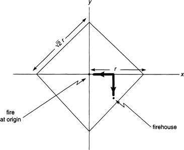
FIGURE 3.1 The right-angle distance metric showing a fire incident at the center, a firehouse, and a right-angle travel path from the firehouse to the incident (as dark line).
If the travel speed of a fire truck is roughly constant, then response time is proportional to travel distance, and so from now on we work with distance traveled rather than elapsed time.
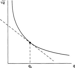
At this juncture, we are able to compute the probability distribution of the travel distance D1 between an incident and the closest responding fire company (see Figure 3.2 for an illustration of a typical situation). Choose the coordinate system so that the incident is located at the origin. Since firehouses are Poisson-distributed in the region, the probability that no fire company is within a distance r of the incident is simply ![]() , using the fact that area in the right-angle metric is 2r2. Therefore the probability that the closest unit is within a distance r is given by
, using the fact that area in the right-angle metric is 2r2. Therefore the probability that the closest unit is within a distance r is given by
![]() (3.6)
(3.6)
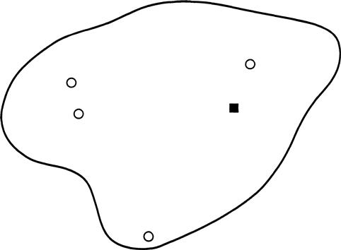
FIGURE 3.2 A hypothetical region with Poisson-distributed fire companies (open circles) and an incident (dark square).
The density function of the random variable D1 is obtained from (3.6) by differentiating F(r) and is given by ![]() . The expected value of D1 is now computed by the integral
. The expected value of D1 is now computed by the integral
 (3.7)
(3.7)
which is evaluated by rewriting (3.7):
Now make the substitution ![]() to obtain
to obtain
and from a table of integrals we find that the last integral has the value ![]() . Putting all this together gives
. Putting all this together gives
![]() (3.8)
(3.8)
We therefore see that the expected travel distance is inversely proportional to the square root of the density of available units. This relation persists under a variety of assumptions about the distribution of response vehicles in the region and the metric one employs. It even continues to be valid if the kth-closest fire company is dispatched instead of the nearest one. We can see this easily enough in the case of D2, the distance to the second-closest unit. The probability that the second closest is within a distance r of an incident, using the right angle metric as before, is 1 minus the probability that either none or exactly one unit is within r. From the Poisson assumption about the distribution of firehouses we obtain
![]()
with a density function given by ![]() .
.
A computation like that given earlier yields
![]() (3.9)
(3.9)
Therefore, except for a slightly larger constant of proportionality, the expected value is the same as (3.8).
Formula (3.8) was derived assuming a right angle distance metric. Using very similar arguments, we can derive the expected value of D1 in terms of the Euclidean metric, in which the distance between two points in the plane is the square root of the sum of the squares of the distances along each coordinate direction. In fact, F(r) = prob(D1 ≤ r) = 1 – e–γπr2, and so ![]() . Make the change of variable x = (γπ)1/2r to obtain
. Make the change of variable x = (γπ)1/2r to obtain
![]()
Because γ = N/A(S), we can rewrite expressions (3.8) and (3.9) as c1/N1/2 and c2/N1/2 for suitable constants, to make the dependence on N more explicit. These mean values assume that all N units are available to respond, which is unrealistic since some fire companies could be busy on other calls. Let m be the number of busy units. In Section 3.2 we showed that the mean of the random variable m is λ/μ, and so the expected value of the variable q = N – m is E(q) = N – λ/μ. Conditioning on q, the number of units actually available, the expectation of D1 is given by
![]()
It is a standard result in probability theory that the unconditional mean of D1 is the average of E(D1|q) with respect to q, namely,
![]()
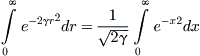
Now, 1/q1/2 is, for q > 0, a convex function, meaning that the tangent line to the curve defined by the graph of the function lies on or below the curve itself (Figure 3.3). Using simple calculus we can show that, because of the convexity,
![]() (3.10)
(3.10)
If we are willing to hazard a possibly low estimate for the mean of D1, then the inequality in (3.10) can be replaced by an equality to give an expression for E(D1) in terms of the average number of available units:
![]() (3.11)
(3.11)
The same relation holds for D2, except the constant is replaced by c2.
Empirical verification of (3.11) has been obtained by plotting actual response-time data against the number of available units (see the paper by Kolesar and Blum [73]), and it is remarkable that the relation persists in spite of the several tenuous assumptions that were made in its derivation, some acceptable, others perhaps less so, such as constant vehicle speed, uniform alarms in space, exponential service times, and a rectangular street grid. The robustness of (3.11) under a variety of conditions compels us to call it the inverse square-root law, and it provides a simple link between available firefighting resources and the ability to respond to an alarm.
3.4 The Encumbrance of an Urban Grid
Since actual travel distances are between the two extremes of Euclidean distance and right-angle distance, aligned along the coordinate north–south axis, it is useful to compute the average travel distance assuming the street network grid is oriented randomly with respect to the coordinate axis.
To carry out this computation, consider two points (x1, y1) and (x2, y2) in the plane and the Euclidean distance between them, as shown in Figure 3.4. Also exhibited there is the path formed according to the right-angle metric, which is oriented at an angle φ relative to the shorter Euclidean path. The total length of this right-angle path is readily seen to be the Euclidean distance times cos φ + sin φ and, therefore, the ratio R of right-angle distance to Euclidean distance is simply cos φ + sin φ.
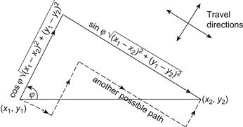
Using a standard trigonometric formula, cos(φ – π/4) = cos φ cos π/4 + sin φ sin π/4 = (cos φ + sin φ)/√2. Thus, R = √2 cos(φ – π/4).
We now compute the probability distribution FR(r) = prob(R ≤ r) = prob(√2 cos(φ – π/4) ≤ r). The event corresponding to R ≤ r is shown in Figure 3.5, in which we assume that the angle φ is uniformly distributed between its minimum and maximum values, namely, 0 ≤ φ ≤ π/2. This means that the density function of φ is 2/π on this interval.
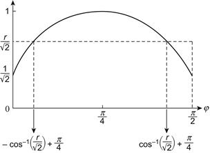
A glance at Figure 3.5 suffices to convince us that R ≤ r is tantamount to φ ≤ – cos–1(r/√2) + π/4 and φ ≥ cos–1(r/√2) + π/4, and so, for 1 ≤ r ≤ √2, (π/2)FR(r) = 1 – 4/π cos–1(r/√2) cos–1(r/√2) + π/4. Note, as required, that FR(1) = 0 and FR(√2) = 1. The density function is dFR(r)/dr = 4/π(2 – r2)–1/2, and from this expression we compute the average value of R:
![]() (3.12)
(3.12)
Thus, on average, the travel distance of a vehicle in an urban street network laid out in grid form is about 1.273 times the Euclidean distance.
3.5 Equilibrium States
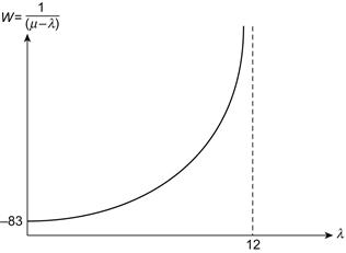
We begin with a true story. In 1972 I was part of a group of consultants to the New York City Sanitation Department under the administration of Mayor John Lindsay. Among the many projects designed to improve the effectiveness of the city’s refuse collection and disposal services, we found ourselves trying to convince the commissioner of sanitation that an increase in the arrival of garbage trucks at a certain dumping facility during peak hours (as a result of a cost-cutting initiative to close another nearby dump) would lead to a disastrous increase in waiting times for the vehicles on line to dump their loads. He thrust aside our written explanations impatiently. After all, the issue was clear to him. The closure he had proposed increased the arrival rate of trucks at the remaining dumpsite by only about 10%, according to the data in our report, and that would therefore increase the waiting time by 10% as well, an acceptable trade-off. Was that really the case? At this juncture we scrapped the written report and drew a simple graph; he immediately appreciated our recommendation to stagger the arrival times of the trucks so as not to increase the average arrival rate during peak hours. What did we show him, and why was it so revealing?
Before getting to that, I need to give a little background by discussing what is arguably the simplest model of a queuing system, one that will be needed in the subsequent section. Customers (refuse trucks, in the present case) randomly arrive at a service facility (the dumpsite) according to a Poisson process at an average rate of λ. They wait in line while an individual within the facility is being serviced (for us, this means that first the vehicles are weighed and then they maneuver into the dumpsite to unload). Immediately after service, the individuals leave. Our assumption is that the completion of service is also a Poisson process at mean rate μ. Let pn(t) be the probability that there are n individuals either waiting on line or in service at time t. To simplify matters, we allow the waiting line to be arbitrarily long, and so there is potentially an infinitude of states in the queue, namely, the number of entities waiting or in service. From state n, two independent events can take place. Either a departure or an arrival occurs at time t. Arrivals happen, according to the fourth assumption, with a probability λh + o(h), and departures happen with probability μh + o(h). The first takes the system from state n to state n + 1, while the second transition moves the system from n to n – 1. We now make another simplifying assumption, namely, that the queue has reached an equilibrium in which the number of arrivals is balanced exactly by the number of departures. During periods of peak activity, after the initial transient fluctuations have damped down, this condition is roughly met, provided μ exceeds λ (otherwise the line grows arbitrarily long) and there are no external disturbances that would serve to invalidate this steady-state condition. Thus, to a close approximation, the probability of finding the system in a particular state no longer varies with the time at which transitions from state to state occur. Accepting this, we can apply some heuristic reasoning to simplify our discussion. First, if the time-independent probability of being in state n is written simply as pn, then it is reasonable to assume that pn is the fraction of time that the system resides in state n.
The equilibrium flow between states depends on whether a new arrival takes place, at rate λ, or a busy unit has terminated service, at rate μ. The probabilities of moving into or out of state n > 0 are independent of time, and the total flow into and out of a given state must be conserved. For example, the rate at which state 1 changes into either state 0 or state 2, namely, (λ + μ), must equal the rate λ into 1 from 0 plus the rate μ from 2 into 1. Then the appropriate balance relation for state 1 is (λ + μ)p1 = λp0 + μp2 because the average transition between states is proportional to the fraction of time the system is actually in each of these states. To see this in the simplest case, suppose that on average there are λ = 12 arrivals per hour and that p0 is 1/4. The flow rate out of state 0 into state 1 is then 12 times p0, namely, three per hour. In this instance, the only departures are from state 1 into state 0, and, since the probabilities must sum to unity, p1 = 3/4 and the flow rate out of 1 into 0 is μ times 3/4, which means that μ must equal four departures per hour. The same argument applies to all the other states and we obtain
![]() (3.13)
(3.13)
![]()
The relations in (3.13) can be solved recursively to obtain pn. First, p1 = (λ/μ)p0. From this, we get p2 = (λ/μ)2p0 and so on, giving pn = (λ/μ)np0 for all n. Since the probabilities pn must sum to 1, it is easily seen that pn = (1 – λ/μ)(λ/μ)n. The average number of individuals on line or in service can be calculated as L = ∑npn summed from 1 to infinity, and this becomes a geometric series that sums to λ/(μ – λ).
The heuristic argument that leads to (3.13) can be given a satisfactory proof (as, for example, in Ross [100]), but what we have suffices to complete the story of the sanitation commissioner. Since L = λW, where W is the average waiting time of a vehicle (see the next paragraph), then W = 1/(μ – λ). A plot of W versus λ for a given value of μ is given in Figure 3.6, where we see that W becomes rapidly unbounded as λ approaches μ. If, for instance, μ = 12 and λ = 10, then a 10% increase in this arrival rate results in more than a 100% increase in W (it doubles). When presented with this simple plot, the commissioner immediately understood the clear conclusion: during periods of high arrivals, waiting time is decidedly nonlinear. His intuition of a proportional increase would be quite reasonable in other circumstances, of course, but in this instance the insertion of randomness led to a strikingly unanticipated result. These elementary considerations from queuing theory are the basis for the remaining discussion in this section
The relation L = λW can be given an intuitive justification for queues in equilibrium. W is the total average time spent by an individual in waiting or in service. Since there are λ arrivals per unit time, then, during W, an average of λW individuals can be found in line or in service, and this is L.
There is a link, of course, between the notion of state transitions given here and those we encountered for Markov chains in Chapter 1, but this would take us beyond what we need here.
3.6 How Busy are the Fire Companies?
Suppose that a district has S fire companies situated within its boundary. When there is a serious multiple-alarm blaze it is conceivable that all these firefighting units would be simultaneously occupied in an attempt to contain the conflagration. During this time, any additional calls for service would have to be handled by more distant units from outside the district, if any are available, and the response time would be longer than usual.
Events that actually strip a district of its firefighting resources are not that unusual in a large city. An explosion in a factory that rages out of control is an example, and the many fires deliberately set during an urban riot is another. Under circumstances like these, it is of interest to know what the probability would be that all S units are busy and, hence, unavailable to other alarms.
To set up the framework for our analysis of this problem, we consider first the simpler case in which exactly one unit is dispatched immediately to each call. In this setting, the number of alarms being serviced is identical to the number of busy fire companies, which virtually excludes from consideration all serious alarms that require multiple servers. We then consider the more realistic situation in which alarms pass through stages. A stage is a period of time during which a fixed number of fire engines are busy at a given incident. When a small fire occurs, for example, three engines might be dispatched and then two released as soon as the first one arrives at the scene and determines that the fire is not serious. Such an incident has two stages. The first stage represents the time until the first engine arrives after receipt of an alarm. The second stage represents the remainder of the incident and has one busy engine. A large fire can generate many stages. For example, suppose that three are initially dispatched. When the first unit arrives at the scene, it determines that the fire is serious and calls for two more units. This initiates a second stage. When the fire is brought under control, four out of the five busy units can be released, allowing a single unit to complete the mop-up operations. The moment of release is the beginning of a third and final stage. It is apparent, then, that the number of busy fire companies at any time is not necessarily the same as the number of fires in progress.
Let us begin with single-stage fires that engage only one firefighting unit. When the fire is serious, what would actually happen is that the first unit arrives and then calls for an additional k – 1 units to be sent to the same location. But, for the sake of simplicity, we temporarily set k equal to unity and collapse the separate stages into a single one.
The ensuing discussion will use the material in Section 3.5 as a point of departure. We assume, as usual, that alarms arrive as a Poisson process at mean rate λ and that the time each fire company is busy on a call is exponential at rate μ. A simplifying assumption is also made that the system of alarms and responses has reached a steady state. This merely paraphrases the equilibrium condition expressed in Section 3.5 that during peak alarm periods the average number of incoming alarms is balanced by the average number of service departures. We use this to imply that the probability of finding exactly k busy units is independent of time. In effect we have a Markov chain in which the long-term probability of finding the system in a particular state no longer varies with the time at which transitions take place. Whether it is in fact possible to disregard fluctuations in these probabilities depends on whether the peak alarm period lasts long enough to ignore initial transient effects and whether there are no unexpected disruptions to service in the interim.
The number of busy fire companies is 0, 1, . . . , S, and we agree to call these the states of the fire-response system. When state S is attained, no additional alarms can be serviced within the district, and, as far as we are concerned, these may be considered “lost” calls. Transitions between states are computed by using the equilibrium hypothesis. Consider the transition diagram shown in Figure 3.7, which expresses the “flow” between states, depending on whether a new alarm has been received at rate λ or a busy unit has completed service at rate μ and is then again available to respond to other calls.
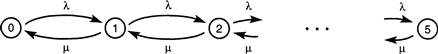
FIGURE 3.7 Transition diagram of flow between states that represent the number of busy fire companies.
In an equilibrium setting, the total flow into and out of a given state must be conserved. For example, the rate at which state 1 changes into either state 0 or state 2, namely, λ + μ, must equal the rate λ into 1 from 0 plus the rate 2μ from 2 into 1. If pk denotes the probability of being in state k, then the appropriate balance relation for state 1 is that (λ + μ)p1 = λp0 + 2μp2, because this conditions the average transitions between states on the probability of actually being in those states. The same argument applies to all other states, and one obtains
![]()
![]() (3.14)
(3.14)
The system of equations (3.14) is easily solved recursively by writing p1 in terms of p0 and then p2 in terms of p1 and so forth. From this we get pk = ρkp0/k!, where ρ = λ/μ. Because the system must be in exactly one of the given states, the pk must sum to unity, and from this we find that
![]() (3.15)
(3.15)
When k is large enough, the sum can be approximated by an exponential, and we obtain the Poisson approximation
![]() (3.16)
(3.16)
In particular, the probability that all S units are busy simultaneously is obtained by letting k = S. Because the distribution of busy units is Poisson, it follows that the mean number of busy units is just ρ. Table 3.1 computes pk from (3.16) for a district having S = 15 units. The mean arrival rate is taken to be eight calls per hour, and service time averages 60 minutes, and so ρ = 8.
TABLE 3.1
Values of pk for a District with S = 15 Units
| k | pk |
| 0 | .0003 |
| 5 | .0916 |
| 8 | .1396 |
| 10 | .0993 |
| 12 | .0481 |
| 15 | .0090 |
The probability peaks at k = 8, which is also the average number of busy units.
Now consider the somewhat more realistic situation where there are two stages and two units are sent initially to every alarm followed by the release of one unit when the fire appears to be still smoldering but under control. The service times in each stage (that is, the duration of the alarms in progress in each stage) are exponential at rates μ1 and μ2, and these are deemed to be independent of each other. Stage 1 occurs when an alarm arrives as a Poisson distribution at rate λ, and stage 2 begins when one of the two busy units terminates its service. The output from stage 1 is the input to stage 2, and to apply the foregoing analysis we must be sure that the input to the second stage is itself Poisson at the same rate so that what we have in effect are two independent Poisson processes in tandem. This is the case, in fact, as sketched in Section 3.8.
There is a trade-off between sending two units initially and finding that only one is needed and initially sending only one unit to a fire that may in fact be serious. In the first instance, one of the units is temporarily unavailable to respond elsewhere, whereas in the other situation there is a delay before a much-needed second unit finally arrives. The delay in the availability of firefighting units increases the risk of loss of life and property.
To analyze the two-stage system, we define states by the doublet (n, m) for non-negative integers n, m, in which n is the number of alarms in progress in stage 1 and m is the number of alarms in progress in stage 2. The phrase “in progress” means that the alarms are being serviced by one or two fire units, whatever the case may be. The transition diagram for the flow between states is shown in Figure 3.8, and Figure 3.9 presents a “close-up” view of the flow into and out of a generic state (n, m).

FIGURE 3.8 Transition diagram of flow between states that represent the number of alarms in progress in each of two stages.
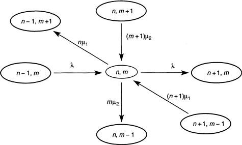
FIGURE 3.9 A close-up view of the diagram in Figure 3.8 showing the flow into and out of a generic state.
Let p(n, m) be the equilibrium probability of finding the fire-response system in state (n, m). Then, just as we did before, the following balance relations for the flow in and out of any state can be read from Figure 3.9:
![]()
for n, m ≥ 1. Similar relations hold when either n or m is zero.
Because there are two units operative in stage 1 and one in stage 2, there will be k busy units altogether whenever n and m satisfy the relation 2n + m = k. Therefore the equilibrium probability pk of finding exactly k busy fire companies is given by
![]() (3.17)
(3.17)
where the double sum is over all n, m for which 2n + m = k. The two stages represent independent firefighting events with Poisson arrivals and exponential service, and so, for all S large enough, the probability of n alarms in progress in stage 1 and m in stage 2 can be approximated by Poisson distributions, by the same reasoning used earlier leading to (3.15). Because of independence, p(n, m) is the product of the separate distributions, and therefore
![]() (3.18)
(3.18)
where r = ρ1 + ρ2, ρ1 = λ/μ1, and ρ2 = λ/μ2. An easy computation reveals that (3.18) satisfies the balance relations shown. The value of pk is now, from (3.17) and (3.18),
![]()
where, once again, the double sum extends over all n, m such that 2n + m = k. In particular, when k = S we get the probability that all available fire companies are busy simultaneously. Table 3.2 gives the values of pk when S = 15, as before, but with an assumption of 45 minutes service time in stage 1 and 15 minutes in stage 2 for a total of 60 minutes. Thus ρ1 = 6 and ρ2 = 2 and r = 8.
TABLE 3.2
Values of pk for a District with S = 15 Units
| k | pk |
| 0 | .0003 |
| 5 | .0251 |
| 8 | .0792 |
| 10 | .1206 |
| 12 | .1494 |
| 13 | .1560 |
| 15 | .1508 |
The probabilities peak at k = 13 at a higher value than that obtained for the single-stage fire treated earlier. Also, the likelihood that all 15 fire companies are busy simultaneously is now .1508, which is a roughly 17-fold increase over the same probability (see Table 3.2) when there are no serious fires requiring multiple servers.
Let us enlarge on this observation. In the multiple-dispatch strategy, two units are sent, so the alarm rate is now effectively doubled as compared to the situation in which a single unit responds to each alarm. If the second stage is discounted, then the average number of busy units is also doubled. This is another way of stating that the likelihood of stripping the region of all its firefighting resources increases when there are multiple stages in which several units can be busy at once.
3.7 Optimal Deployment of Fire Companies
A city has been partitioned into k districts; within each of these, fire alarms occur at random in a spatially uniform manner. These homogeneous sectors represent the different alarm histories that one can expect in diverse parts of the overall region, such as high- and low-density residential and business zones, where hazard rates vary with locale. Some sectors may also be determined by geography, as, for example, when a river forms a natural barrier that separates one zone from another.
Calls in district i are assumed to come from a Poisson distribution at rate λi, i = 1, 2, . . . , k. The probability that the next citywide alarm actually originates from district i is, from Lemma 3.2, λi/λ, where λ is the sum of λ1 through λk. For each i, let Ni be the number of fire companies assigned to the ith district and let μi be the average service time of companies in that district, which depends on travel conditions and the severity of fires. Service times are exponentially distributed.
Conditioning on the k disjoint events that an alarm arrives from sector i, the region-wide unconditional response distance D to the closest responding unit (our surrogate for response time) has an expected value that can be computed from formula (3.11):
![]() (3.19)
(3.19)
where ci equals 0.627 times the square root of the area of sector i. The fire department would like E(D) to be as small as possible, and this leads to the optimization problem of minimizing this sum subject to the conditions that the Ni add up to N, the total available resources in the city, and that Ni are integers, at least 1 greater than the smallest integer in λi/μi. Once again, as in Chapter 2, this is an integer program, and it admits a simple solution. One begins by assigning the smallest possible number of units, 1 + λi/μi, to the ith term in (3.19). If this bare-bones deployment adds up to N, we are done. Otherwise, allocate one more unit to that term for which g(Ni) – g(Ni + 1) is largest, because this choice decreases the sum the most. Continue in this fashion until all N available units have been assigned.
The resulting allocation is designed to optimize the citywide efficiency of deployment, but it may suffer in other respects. For example, a high-demand area with many fire alarms would receive somewhat more companies than would an adjacent sector that has fewer alarms, such as a low-density residential part of town. However, when a fire does occur in the residential area, the response time is likely to be greater, since the responding units are more dispersed. The tax-paying residents are understandably resentful of this inequity in coverage because they are being penalized for having fewer fires. Suppose then, in response to their outcry, that some additional units are shifted permanently to the residential zone. This leaves the high-density area more vulnerable than before, since travel times would tend to increase and, what is perhaps of equal significance, the workload of the fire companies in the high-demand area would exceed that of the companies in the adjoining region, in the sense that each is busier a greater fraction of the time. The firefighters’ union would protest.
There is an evident need to reconcile the multiple and often-conflicting interests of the city administration, the employees union, and community groups. Although the citywide allocation based on the inverse square-root law may fail adequately to meet the criteria of fairness imposed by citizens and firefighters (equity of coverage and equity of workload), it provides a compromise by placing more units in the high-demand areas while ensuring an acceptable level of coverage, and it has been used effectively by several municipalities as a rule of thumb for resource allocation. In New York City, for instance, during one of its recurrent fiscal crises, the fire department budget was cut and some fire companies had to be disbanded. Other units were then relocated to fill the resulting gaps in coverage by employing the inverse square-root law to minimize the degradation in service caused by the cuts.
These changes were initially resisted by the firefighters as well as by community groups that felt threatened by the moves, but ultimately the cost-saving measures were implemented (for further comments on this, see Section 3.8).
One way to achieve equity of coverage is temporarily to reposition fire companies to other houses during periods of heavy demand. This relieves busy units and tends to reduce workload imbalances as well. The repositioning problem can be formulated mathematically by first partitioning a region into subzones called “response neighborhoods,” each of which is served by the two closest fire companies. Some firehouses may, of course, belong to more than one response neighborhood, assuming one company per firehouse, and so the partition consists of overlapping subzones.
A response neighborhood is uncovered if both of its closest units are busy on other calls, in which case some other available unit is assigned temporarily to one of the empty firehouses (Figure 3.10). The problem now is to decide which of the empty houses to fill so as to minimize the number of relocated companies. The issue here is not which of the available units to reposition but, rather, how many, and is reminiscent of the integer programming problems considered in the previous chapter.
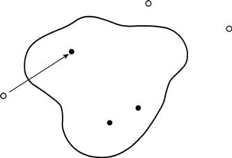
FIGURE 3.10 Illustration of repositioning with one unprotected response neighborhood and several adjacent firehouses.
The dark circles are empty firehouses, and the open circles designate firehouses with an available unit. The arrow shows a deployable company being moved, temporarily, to the empty firehouse of a busy company.
Part of the appeal of the inverse square-root law is that, although it is deceptively simple to state and to use, it is a surprisingly effective tool for planning the long-term deployment of firefighting resources. However, there are other short-term deployment issues concerning day-to-day operations that are also of considerable interest, and we touch on them briefly next.
Although we have assumed that one always dispatches the nearest unit to an alarm, it is not obvious that sending a more distant unit could sometimes be more effective in the long run. Usually the optimal response is to deploy the closest unit (or units). But during a busy period in a high-demand area, this dispatch policy could strip the immediate area of all its firefighting resources, and a future alarm might well be answered by a unit that is considerably more distant. Therefore, if the closest unit is not dispatched initially to an alarm, the delay in response experienced by the incident could be compensated for by the ability of that unit to be available to handle a future alarm. There is a trade-off here between the short-term advantage in responding quickly to a current alarm and the long-term gain in having units available to send to future incidents. The problem is to decide on how to place the boundary of the response sector of a first responding unit so that an exceptionally busy company has a smaller response zone than would a company in a lower alarm area. With appropriately redefined boundaries, any workload imbalance is reduced, and there would be an occasional exception to the rule of sending the closest unit (see Figure 3.11 for an illustration of this idea). This is in contrast to the repositioning problem considered earlier, in which boundaries were drawn specifically to include the closest (and second-closest) units.
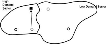
FIGURE 3.11 Adjacent high- and low-demand areas, with the boundary between them drawn so that the first responding unit is not necessarily the closest unit.
The open circles are available firehouses, and the dark square is an incident. The arrow shows a deployable company responding to the incident.
These tactical questions of how many and which units to dispatch can be formulated mathematically, but we do not do so here (see, however, the references in Section 3.8).
3.8 Concluding Thoughts
Optimization of the citywide deployment of fire companies using formula (3.19) guarantees a level of efficiency that slights other considerations of equity, as discussed in Section 3.7. A modification of (3.17) offers a partial way out of the dilemma. Replace each of the expressions (Ni – λi/μi)–1/2, which we rewrite as gi(Ni) for short, by gi(Ni)b, where b is a non-negative parameter. When b = 1, one recovers (3.19); but if b is taken to be smaller than 1, then each term in the sum becomes less dependent on response distance, especially as b gets closer to zero. On the other hand, when we choose b to be greater than 1, the opposite occurs, and, as b gets larger and larger, the terms with the larger travel distances begin to dominate the sum. These conflicting measures of performance—namely, efficiency of coverage, workload imbalance, and coverage imbalance, all discussed in Section 3.7—can be traded off against each other by letting b vary over non-negative values.
In Section 3.6 we used the fact that the output of a Poisson arrival queue with exponentially distributed service is again Poisson, and so, in a two-stage queue, the output of the first server can be considered a Poisson input to the second stage. An intuitive proof of this comes by considering a queuing system with a single Poisson input at mean rate λ and exponential service with mean interservice times 1/μ, which spews out a departure stream that, viewed in reverse, may be considered as arrivals to the same system from the backdoor, so to speak. The service rate remains μ, and the departures from this reversed system form what we know to be a Poisson process at rate λ. In a steady state it is reasonable to assume that these processes are mirror images of each other, and this implies that the output of the original queuing system must indeed be Poisson at rate λ. That departures can be viewed as arrival in reverse is a paraphrase of what is known as Burke’s Theorem [27].
There are a number of books on stochastic processes that discuss the Poisson distribution in detail, at a level commensurate with that adopted in this chapter. We can recommend the most recent edition of a book by Ross [100].
The inverse square-root law for fire department operations was derived and tested by Kolesar and Blum [73]. A more comprehensive discussion of the models employed in this chapter, together with a thorough treatment of the Rand Fire Study, with further references, is in the book edited by Walker et al. [114]. This includes the question of which units to deploy to a given alarm and the issue of how many to dispatch. The deployment of fire companies in multiple stages, the topic of Section 3.4, is due to Jan Chaiken and can be found in his report [31] and in Chapter 7 of the book by Walker et al. [114] just referenced.
As noted previously, the inverse square-root law was a key tool in deciding how many fire companies to disband and how many to relocate during the fiscal crisis of New York City in 1971. This controversial move engendered protests at city hall and a suit in federal court by the firefighters’ union and by irate citizens. However, after the analysis was explained in court and at briefings to local groups, the opposition died down and the changes took place at a considerable saving to the city (see “Union Fights Fire Department Cuts,” New York Times, December 22, 1972).