
Chapter 5
Collectives
In Chapter 4, we introduced the map pattern, which describes embarrassing parallelism: parallel computations on a set of completely independent operations. However, obviously we need other patterns to deal with problems that are not completely independent.
The collective operations are a set of patterns that deal with a collection of data as a whole rather than as separate elements. The reduce pattern allows data to be summarized; it combines all the elements in a collection into a single element using some associative combiner operator. The scan pattern is similar but reduces every subsequence of a collection up to every position in the input. The usefulness of reduce is easy to understand. One simple example is summation, which shows up frequently in mathematical computations. The usefulness of scan is not so obvious, but partial summarizations do show up frequently in serial algorithms, and the parallelization of such serial algorithms frequently requires a scan. Scan can be thought of as a discrete version of integration, although in general it might not be linear.
As we introduce the reduce and scan patterns, we will also discuss their implementations and various optimizations particularly arising from their combination with the map pattern.
Not included in this chapter are operations that just reorganize data or that provide different ways to view or isolate it, such as partitioning, scatter, and gather. When data is shared between tasks these can also be used for communication and are will be discussed in Chapter 6.
5.1 Reduce
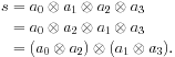
In the reduce pattern, a combiner function ![]() is used to combine all the elements of a collection pairwise and create a summary value. It is assumed that pairs of elements can be combined in any order, so multiple implementations are possible. Possible implementations of reduce are diagrammed in Figure 5.1. The left side of this figure is equivalent to the usual naive serial implementation for reducing the elements of a collection. The code given in Listing 5.1 implements the serial algorithm for a collection a with n elements.
is used to combine all the elements of a collection pairwise and create a summary value. It is assumed that pairs of elements can be combined in any order, so multiple implementations are possible. Possible implementations of reduce are diagrammed in Figure 5.1. The left side of this figure is equivalent to the usual naive serial implementation for reducing the elements of a collection. The code given in Listing 5.1 implements the serial algorithm for a collection a with n elements.
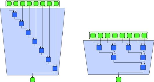
Figure 5.1 Serial and tree implementations of the reduce pattern for 8 inputs.
The identity of the combiner function is required by this implementation. This is so that the reduction of an empty collection is meaningful, which is often useful for boundary conditions in algorithms. In this implementation the identity value could also be interpreted as the initial value of the reduction, although in general we should distinguish between initial values and identities. If we do not need to worry about empty collections, we can define the reduce pattern using Listing 5.2.
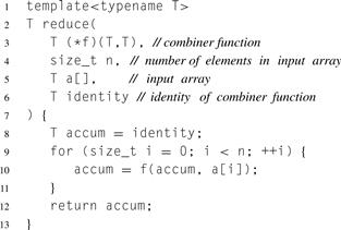
Listing 5.1 Serial reduction in C++ for 0 or more elements.
5.1.1 Reordering Computations
To parallelize reduction, we have to reorder the operations used in the serial algorithm. There are many ways to do this but they depend on the combiner function having certain algebraic properties.
To review some basic algebra, a binary operator ![]() is considered to be associative or commutative if it satisfies the following equations:
is considered to be associative or commutative if it satisfies the following equations:
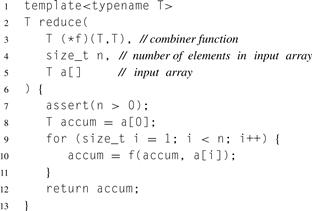
Listing 5.2 Serial reduction in C++ for 1 or more elements.
Associativity and commutativity are not equivalent. While there are common mathematical operations that are both associative and commutative, including addition; multiplication; Boolean AND, OR, and XOR; maximum; and minimum (among others), there are many useful operations that are associative but not commutative. Examples of operations that are associative but not commutative include matrix multiplication and quaternion multiplication (used to compose sequences of 3D rotations). There are also operations that are commutative but not associative, an example being saturating addition on signed numbers (used in image and signal processing). More seriously, although addition and multiplication of real numbers are both associative and commutative, floating point addition and multiplication are only approximately associative. Parallelization may require an unavoidable reordering of floating point computations that will change the result.
To see that only associativity is required for parallelization, consider the following:
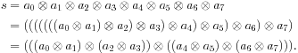
The first grouping shown is equivalent to the left half of Figure 5.1, the second grouping to the right right half of Figure 5.1. Another way to look at this is that associativity allows us to use any order of pairwise combinations as long as “adjacent” elements are intermediate sequences. However, the second “tree” grouping allows for parallel scaling, but the first does not.
A good example of a non-associative operation is integer arithmetic with saturation. In saturating arithmetic, if the result of an operation is outside the representable range, the result is “clamped” to the closest representable value rather than overflowing. While convenient in some applications, such as image and signal processing, saturating addition is not associative for signed integers.
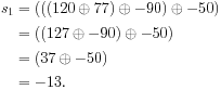
The following example shows that saturating addition is not associative for signed bytes. Let ⊕ be the saturating addition operation. A signed byte can represent an integer between −128 and 127 inclusive. Thus, a saturating addition operation 120 ⊕ 78 yields 127, not 198. Consider reduction with ⊕ of the sequence [120, 78, −90, −50]. Serial left-to-right order yields:
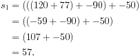
Tree order yields a different result:
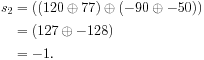
In contrast, modular integer addition, where overflow wraps around, is fully associative. A result greater than 127 or −128 is brought in range by adding or subtracting 256, which is equivalent to looking at only the low-order 8 bits of the binary representation of the algebraic result. Here is the serial reduction with modular arithmetic on signed bytes:
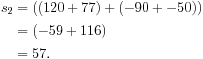
Tree ordering gives the same result:
5.1.2 Vectorization
There are useful reorderings that also require commutativity. For example, suppose we want to vectorize a reduction on a processor with two-way SIMD instructions. Then we might want to combine all the even elements and all the odd elements separately, as in Figure 5.2, then combine the results. However, this reordering requires commutativity:
Note that a1 and a2 had to be swapped before we could group the operations according to this pattern.
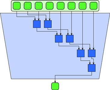
Figure 5.2 A reordering of serial reduction that requires commutativity. Commutativity of the combiner operator is not required for parallelization but enables additional reorderings that may be useful for vectorization. This example reduces eight inputs using two serial reductions over the even and odd elements of the inputs then combines the results. This reordering is useful for vectorization on SIMD vector units with two lanes.
5.1.3 Tiling
In practice, we want to tile1 computations and use the serial algorithm for reduction when possible. In a tiled algorithm, we break the work into chunks called tiles (or blocks), operate on each tile separately, and then combine the results. In the case of reduce, we might want to use the simple serial reduce algorithm within each tile rather than the tree ordering. This is because, while the tree and serial reduce algorithms use the same number of applications of the combiner function, the simplest implementation of the tree ordering requires O (n) storage for intermediate results while the serial ordering requires only O (1) storage.
This is shown in Figure 5.3 for 16 inputs with four tiles of four inputs each, followed by a “global reduction” with four inputs. In practice, since synchronization is expensive, it is common for reductions to have only two phases: a local phase over tiles and a global phase combining the results from each tile. We may also use a vectorized implementation within the tiles as discussed in Section 5.1.2, although this usually requires further reordering.
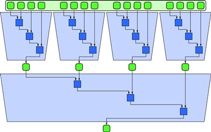
Figure 5.3 A reordering of reduction using serial reductions on tiles and then reductions of the results of those reductions. This can be generalized to a two-phase approach to implementing reduce in general.
Warning
The issues of associativity and commutativity matter mostly when the combiner function may be user defined. Unfortunately, it is hard for an automated system to prove that an arbitrary function is associative or commutative, although it is possible to do so in specific cases—for example, when forming expressions using known associative operators [FG94]. Generally, though, these properties have to be asserted and validated by the user. Therefore, you need to make sure that when using user-defined reductions the functions you are providing satisfy the required properties for the implementation. If you violate the assumptions of the implementation it may generate incorrect and/or non-deterministic results. It is also necessary for the implementor of a reduction taking arbitrary combiner functions to document whether or not commutativity is assumed. The issue does not arise when only built-in operations with known properties are provided by the reduction implementor.
5.1.4 Precision
Another issue can arise with large reductions: precision. Large summations in particular have a tendency to run out of bits to represent intermediate results. Suppose you had an array with a million single-precision floating point numbers and you wanted to add them up. Assume that they are all approximately the same magnitude. Single-precision floating point numbers only have about six or seven digits of precision. What can happen in this scenario if the naïve serial algorithm is used is that the partial sum can grow very large relative to the new values to be added to it. If the partial sum grows large enough, new values to it will be less than the smallest representable increment and their summation will have no effect on the accumulator. The increments will be rounded to zero. This means that part of the input will effectively be ignored and the result will of course be incorrect.
The tree algorithm fares better in this case. If all the inputs are about the same size, then all the intermediate results will also be about the same size. This is a good example of how reassociating floating point operations can change the result. Using a tiled tree will retain most of the advantages of the tree algorithm if the tiles and the final pass are of reasonable sizes.
The tree algorithm is not perfect either, however. We can invent inputs that will break any specific ordering of operations. A better solution is to use a larger precision accumulator than the input. Generally speaking, we should use double-precision accumulators to sum single-precision floating point inputs. For integer data, we need to consider the largest possible intermediate value.
Converting input data to a higher-precision format and then doing a reduce can be considered a combination of a map for the conversion and a reduce to achieve the higher-precision values. Fusion of map and reduce for higher performance is discussed in Section 5.2.
5.1.5 Implementation
Most of the the programming models used in this book, except OpenCL, include various built-in implementations of reduce. TBB and Cilk Plus in addition support reduce with user-defined combiner functions. However, it your responsibility to ensure that the combiner function provided is associative. If the combiner function is not fully associative (for example if it uses floating point operations), you should be aware that many implementations reassociate operations non-deterministically. When used with combiner functions that are not fully associative, this can change the result from run to run of the program. At present, only TBB provides a guaranteed deterministic reduce operation that works with user-defined combiner functions that are not fully associative.
OpenCL
Reduce is not a built-in operation, but it is possible to implement it using a sequence of two kernels. The first reduces over blocks, and the second combines the results from each block. Such a reduction would be deterministic, but optimizations for SIMD execution may also require commutativity.
TBB
Both deterministic and non-deterministic forms of reduce are supported as built-in operations. The basic form of reduce is parallel_reduce. This is a fast implementation but may non-deterministically reassociate operations. In particular, since floating point operations are not truly associative, using this construct with floating point addition and multiplication may lead to non-determinism. If determinism is required, then the parallel_deterministic_reduce construct may be used. This may result in lower performance than the non-deterministic version. Neither of these implementations commutes operations and so they can both safely be used with non-commutative combiner functions.
Cilk Plus
Two forms of reduce are provided: __sec_reduce for array slices, and reducer hyperobjects. Both of these support user-defined combiner functions and assume associativity. Neither form assumes commutativity of a user-defined combiner. Either of these reductions may non-deterministically reassociate operations and so may produce non-deterministic results for operations that are not truly associative, such as floating point operations. It is possible to implement a deterministic tree reduction in a straightforward fashion in Cilk Plus using fork–join, although this may be slower than the built-in implementations.
ArBB
Only reductions using specific associative and commutative built-in operations are provided. Floating point addition and multiplication are included in this set. The implementation currently does not guarantee that the results of floating point reductions will be deterministic. If a deterministic reduce operation is required, it is possible to implement it using a sequence of map operations, exactly as with OpenCL.
OpenMP
Only reductions with specific associative and commutative built-in operations are provided. More specifically, when a variable is marked as a reduction variable, at the start of a parallel region a private copy is created and initialized in each parallel context. At the end of the parallel region the values are combined with the specified operator.
5.2 Fusing Map and Reduce
A map followed by a reduce can be optimized by fusing the map computations with the initial stages of a tree-oriented reduce computation. If the map is tiled, this requires that the reduction be tiled in the same way. In other words, the initial reductions should be done over the results of each each map tile and then the reduce completed with one or more additional stages. This is illustrated in Figure 5.4.
Figure 5.4 Optimization of map and reduce by fusion. When a map feeds directly into a reduction, the combination can be implemented more efficiently by combining the map with the initial stage of the reduce.
This optimization avoids the need for a synchronization after the map and before the reduce, and it also avoids the need to write the output of the map to memory if it is not used elsewhere. If this is the case, the amount of write bandwidth will be reduced by a factor equal to the tile size. The synchronization can also be avoided in sophisticated systems that break the map and reduce into tiles and only schedule dependencies between tiles. However, even such systems will have overhead, and fusing the computations avoids this overhead.
5.2.1 Explicit Fusion in TBB
The map and reduce patterns can be fused together in TBB by combining their implementations and basically combining the first step of the reduce implementation with some preprocessing (the map) on the first pass. In practice, this can be accomplished through appropriate use of the tiled reduction constructs in TBB, as we show in Section 5.3.4.
5.2.2 Explicit Fusion in Cilk Plus
In Cilk Plus map and reduce can be fused by combining their implementations. The map and initial stages of the reduce can be done serially within a tile, and then the final stages of the reduce can be done with hyperobjects. We show an example of this in Section 5.3.5.
5.2.3 Automatic Fusion in ArBB
A map followed by a reduce is fused automatically in ArBB. You do not have to do anything special, except ensure that the operations are in the same call. Technically, ArBB does a code transformation on the sequence of operations that within serial code generation is often called loop fusion. In ArBB, however, it is applied to parallel operations rather than loop iterations.
The map and reduce operations do not have to be adjacent in the program text either, as opportunities for fusion are found by analyzing the computation’s data dependency graph. The system will also find multiple fusion opportunities—for example, a map followed by multiple different reductions on the same data. If the output of the map is the same shape as that used by the reduce operations, the fusion will almost always happen. However, intermediate random-memory access operations such as gather and scatter will inhibit fusion, so they should be used with this understanding.
ArBB does not currently provide a facility to allow programmers to define their own arbitrary combiner functions for reductions. Instead, complex reductions are built up by fusing elementary reductions based on basic arithmetic operations that are known to be associative and commutative.
5.3 Dot Product
As a simple example of the use of the different programming models, we will now present an implementation of the inner or “dot” product in TBB, Cilk Plus, SSE intrinsics, OpenMP, and ArBB. Note that this is actually an example of a map combined with a reduction, not just a simple reduction. The map is the initial pairwise multiplication, and the reduction is the summation of the results of that multiplication.
5.3.1 Description of the Problem
Given two vectors (1D arrays) a and b each with n elements, the dot product ![]() is a scalar given by:
is a scalar given by:
![]()
where ai and bi denote the ith elements of a and b, respectively. Subscripts run from 0 to n − 1 as usual in C and C++.
It is unlikely that a scalable speedup will be obtained when parallelizing such a simple computation. As with SAXPY in Section 4.2, a simple operation such as dot product is likely to be dominated by memory access time. The dot product is also the kind of computation where calling a library routine would probably be the best solution in practice, and tuned implementations of the dot product do indeed appear in BLAS libraries. However, dot product is simple and easy to understand and also shows how a map can be combined with reduce in practice.
As map and reduce are a common combination, you can use these examples as templates for more complex applications. We will also use this example to demonstrate some important optimizations of this combination without getting caught up in the complexities of the computation itself.
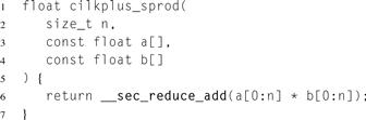
5.3.2 Serial Implementation
For reference, a serial implementation of dot product is provided in Listing 5.3. There is nothing special here. However, note that the usual serial expression of reduce results in loop-carried dependencies and would not be parallelizable if implemented in exactly the order specified in this version of the algorithm. You have to recognize, abstract, and extract the reduce operation to parallelize it. In this case, the serial reduce pattern is easy to recognize, but when porting code you should be alert to alternative expressions of the same pattern.
This example assumes that n is small, so the reduction accumulator can have type float. For large reductions this is unwise since single-precision floating point values may not be able to represent partial sums with sufficient precision as explained in Section 5.1.4. However, the same type for the accumulator, the input, and the output has been used in order to simplify the example. In some of the implementations we will show how to use a different type for performing the accumulations.
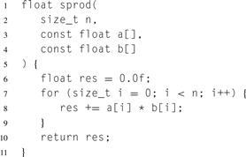
Listing 5.3 Serial implementation of dot product in C++. The reduction in this example is based on a loop-carried dependency and is not parallelizable without reordering the computation.
5.3.3 SSE Intrinsics
Listing 5.4 gives an explicitly vectorized version of the dot product computation. This example uses SSE intrinsics. SSE stands for Streaming SIMD Extensions and is an instruction set extension supported by Intel and AMD processors for explicitly performing multiple operations in one instruction. It is associated with a set of registers that can hold multiple values. For SSE, these registers are 128 bits wide and can store two double-precision floating point values or four single-precision floating point values.
When using SSE intrinsics, special types are used to express pairs or quadruples of values that may be stored in SSE registers, and then functions are used to express operations performed on those values. These functions are recognized by the compiler and translated directly into machine language.
Use of intrinsics is not quite as difficult as writing in assembly language since the compiler does take care of some details like register allocation. However, intrinsics are definitely more complex than the other programming models we will present and are not as portable to the future. In particular, SIMD instruction sets are subject to change, and intrinsics are tied to specific instruction sets and machine parameters such as the width of vector registers.
For (relative) simplicity we left out some complications so this example is not really a full solution. In particular, this code does not handle input vectors that are not a multiple of four in length.
Some reordering has been done to improve parallelization. In particular, this code really does four serial reductions at the same time using four SSE register “lanes”, and then combines them in the end. This uses the implementation pattern for reduce discussed in Section 5.1.2, but with four lanes. Like the other examples that parallelize reduce, some reordering of operations is required, since the exact order given in the original serial implementation is not parallelizable. This particular ordering assumes commutativity as well as associativity.
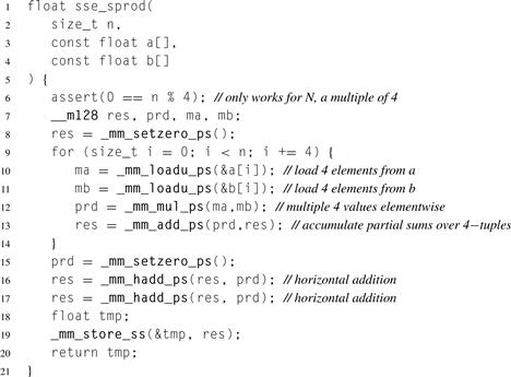
Listing 5.4 Vectorized dot product implemented using SSE intrinsics. This code works only if the number of elements in the input is a multiple of 4 and only on machines that support the SSE extensions. This code is not parallelized over cores.
Other problems with the SSE code include the fact that it is machine dependent, verbose, hard to maintain, and it only takes advantage of vector units, not multiple cores. It would be possible to combine with code with a Cilk Plus or TBB implementation in order to target multiple cores, but that would not address the other problems. In general, machine dependence is the biggest problem with this code. In particular, new instruction set extensions such as AVX are being introduced that have wider vector widths, so it is better to code in a way that avoids dependence on a particular vector width or instruction set extension.
5.3.4 TBB
Listing 5.5 uses TBB’s algorithm template parallel_reduce. This template recursively decomposes a reduction into smaller subreductions and reduces each base case using a functor provided by the user. Here that functor uses std::inner_product to do serial reduction, which the compiler may be able to automatically vectorize. The base case code can also be used for map–reduce fusion, as done here: the std::inner_product call in the base case does both the multiplications and a reduction over the tile it is given. The user must also provide a functor to combine the results of the base cases, which here is the functor std::plus<float>.
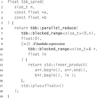
Listing 5.5 Dot product implemented in TBB.
The template parallel_reduce also requires the identity of the combiner function. In this case, the identity of floating point addition is float(0). Alternatively, it could be written as 0.f. The f suffix imbues the constant with type float. It is important to get the type right, because the template infers the type of the internal accumulators from the type of the identity. Writing just 0 would cause the accumulators to have the type of a literal 0, which is int, not the desired type float.
The template parallel_reduce implements a flexible reduce pattern which can be instantiated in a variety of ways. For example, Listing 5.6 shows an instantiation that does accumulation using a precision higher than the type of the input, which is often important to avoid overflow in large reductions. The type used for the multiplication is also changed, since this is a good example of a fused map operation. These modifications change float in Listing 5.5 to double in several places:
2. The identity element is double(0), so that the template uses double as the type to use for internal accumulators.
3. The parameter in is declared as double, not only because it might hold a partial accumulation, but because std::inner_product uses this type for its internal accumulator.
4. To force use of double-precision + and * by std::inner_product, there are two more arguments, std::plus<double>() and std::multiplies<double>(). An alternative is to write the base case reduction with an explicit loop instead of std::inner_product.
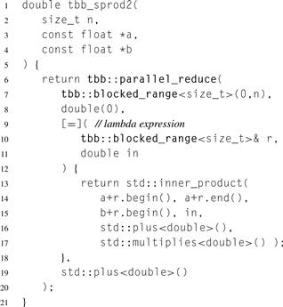
Listing 5.6 Modification of Listing 5.5 with double-precision operations for multiplication and accumulation.
5.3.5 Cilk Plus
Listing 5.7 expresses the pairwise multiplication and reduction using Cilk Plus array notation. A good compiler can generate code from it that is essentially equivalent to the hand-coded SSE in Listing 5.4, except that the Cilk Plus version will correctly handle vector widths that are not a multiple of the hardware vector width. In fact, it is not necessary to know the hardware vector width to write the Cilk Plus code. The Cilk Plus code is not only shorter and easier to understand and maintain, it’s portable.
An explicitly thread parallel and vector parallel dot product can be expressed as shown in Listing 5.8. The variable res has a special type called a reducer. Here the reducer res accumulates the correct reduction value even though there may be multiple iterations of the cilk_for running in parallel. Even though the code looks similar to serial code, the Cilk Plus runtime executes it using a tree-like reduction pattern. The cilk_for does tree-like execution (Section 8.3) and parts of the tree executing in parallel get different views of the reducer. These views are combined so at the end of the cilk_for there is a single view with the whole reduction value. Section 8.10 explains the mechanics of reducers in detail.
Our code declares res as a reducer_opadd<float> reducer. This indicates that the variable will be used to perform + reduction over type float. The constructor argument (0) indicates the variable’s initial value. Here it makes sense to initialize it with 0, though in general a reducer can be initialized with any value, because this value is not assumed to be the identity. A reducer_opadd<T> assumes that the identity of + is T(), which by C++ rules constructs a zero for built-in types. The min expression in the code deals with a possible partial “boundary” tile, so the input does not have to be a multiple of the tile size.
Listing 5.7 Dot product implemented in Cilk Plus using array notation.
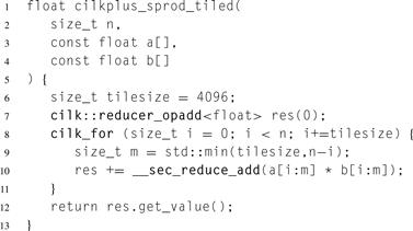
Listing 5.8 Dot product implementation in Cilk Plus using explicit tiling.
Listing 5.8 shows how to modify the reduction to do double-precision accumulation. The casts to double-precision are also placed to result in the use of double-precision multiplication. These casts, like the multiplication itself, are really examples of the map pattern that are being fused into the reduction. Of course, if you wanted to do single-precision multiplication, you could move the cast to after the __sec_reduce_add. Doing the multiplication in double precision may or may not result in lower performance, however, since a dot product will likely be performance limited by memory bandwidth, not computation. Likewise, doing the accumulation in double precision will likely not be a limiting factor on performance. It might increase communication slightly, but for reasonably large tile sizes most of the memory bandwidth used will result from reading the original input.
5.3.6 OpenMP
An OpenMP implementation of dot product is shown in Listing 5.10. In OpenMP, parallelization of this example is accomplished by adding a single line annotation to the serial implementation. However, the annotation must specify that res is a reduction variable. It is also necessary to specify the combiner operator, which in this case is (floating point) addition.
What actually happens is that the scope of the loop specifies a parallel region. Within this region local copies of the reduction variable are made and initialized with the identity associated with the reduction operator. At the end of the parallel region, which in this case is the end of the loop’s scope, the various local copies are combined with the specified combiner operator. This code implicitly does map–reduce fusion since the base case code, included within the loop body, includes the extra computations from the map.
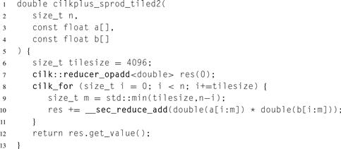
Listing 5.9 Modification of Listing 5.8 with double-precision operations for multiplication and accumulation.
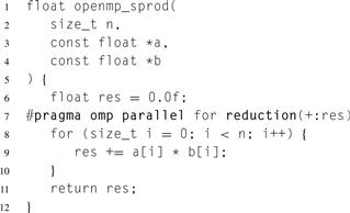
Listing 5.10 Dot product implemented in OpenMP.
OpenMP implementations are not required to inform you if the loops you annotate have reductions in them. In general, you have to identify them for yourself and correctly specify the reduction variables. OpenMP 3.1 provides reductions only for a small set of built-in associative and commutative operators and intrinsic functions. User-defined reductions have to be implemented as combinations of these operators or by using explicit parallel implementations. However, support for user-defined reductions is expected in a future version of OpenMP, and in particular is being given a high priority for OpenMP 4.0, since it is a frequently requested feature.
5.3.7 ArBB
Listing 5.11 gives the kernel of a dot product in ArBB. This function operates on ArBB data, so the additional code in Listing 5.12 is required to move data into ArBB space, invoke the function in Listing 5.11 with call, and retrieve the result with value. Internally, ArBB will generate tiled and vectorized code roughly equivalent to the implementation given in Listing 5.8.
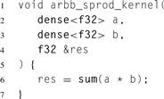
Listing 5.11 Dot product implemented in ArBB. Only the kernel is shown, not the binding and calling code, which is given in Listing 5.12.
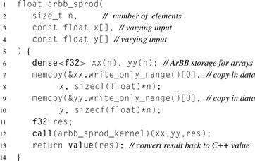
Listing 5.12 Dot product implementation in ArBB, using wrapper code to move data in and out of ArBB data space and invoke the computation.
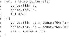
Listing 5.13 High-precision dot product implemented in ArBB. Only the kernel is shown.
To avoid overflow in a very large dot product, intermediate results should be computed using double precision. The alternative kernel in Listing 5.13 does this. The two extra data conversions are, in effect, additional map pattern instances. Note that in ArBB multiple maps are fused together automatically as are maps with reductions. This specification of the computation produces an efficient implementation that does not write the intermediate converted high-precision input values to memory.
5.4 Scan
The scan collective operation produces all partial reductions of an input sequence, resulting in a new output sequence. There are two variants: inclusive scan and exclusive scan. For inclusive scan, the nth output value is a reduction over the first n input values; a serial and one possible parallel implementation are shown in Figure 5.5. For exclusive scan, the nth output value is a reduction over the first n − 1 input values. In other words, exclusive scan excludes the nth output value. The C++ standard library template std::partial_sum is an example of an inclusive scan. Listings 5.14 and 5.15 show serial routines for inclusive scan and exclusive scan, respectively.
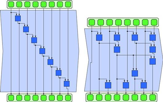
Figure 5.5 Serial and parallel implementations of the (inclusive) scan pattern.
Each of the routines takes an initial value to be used as part of the reductions. There are two reasons for this feature. First, it avoids the need to have an identity element when computing the first output value of an exclusive scan. Second, it makes serial scan a useful building block for writing tiled parallel scans.
At first glance, the two implementations look more different than they really are. They could be almost identical, because another way to write an exclusive scan is to copy Listing 5.14 and swap lines 10 and 11. However, that version would invoke combine one more time than necessary.
Despite the loop-carried dependence, scan can be parallelized. Similar to the parallelization of reduce, we can take advantage of the associativity of the combiner function to reorder operations. However, unlike the case with reduce, parallelizing scan comes at the cost of redundant computations. In exchange for reducing the span from O (N) to O(lg N), the work must be increased, and in many algorithms nearly doubled. One very efficient approach to parallelizing scan is based on the fork–join pattern. The fork–join pattern is covered in Chapter 8, and this approach is explained in Section 8.11 along with an implementation in Cilk Plus. Section 5.4 presents another implementation of scan using a three-phase approach and an implementation using OpenMP.
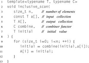
Listing 5.14 Serial implementation of inclusive scan in C++, using a combiner functor and an initial value.
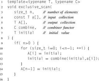
Listing 5.15 Serial implementation of exclusive scan in C++. The arguments are similar to those in Listing 5.14.
Scan is a built-in pattern in both TBB and ArBB. Here is a summary of the characteristics of these implementations at the point when this book was written. We also summarize the interface and characteristics of the scan implementation we will present for Cilk Plus and give a three-phase implementation of scan in OpenMP.
5.4.1 Cilk Plus
Cilk Plus has no built-in implementation of scan. Section 8.11 shows how to implement it using the fork–join pattern. The interface to that implementation and its characteristics are explained here, however, so we can use it in the example in Section 5.6.
Our Cilk Plus implementation performs a tiled scan. It abstracts scan as an operation over an index space and thus makes no assumptions about data layout. The template interface is:
template<typename T, typename R, typename C, typename S>
void cilk_scan(size_t n, T initial, size_t tilesize,
R reduce, C combine, S scan);
The parameters are as follows:
• n is the size of the index space. The index space for the scan is the half-open interval [0, n).
• initial is the initial value for the scan.
• tilesize is the desired size of each tile in the iteration space.
• reduce is a functor such that reduce(i,size) returns a value for a reduction over indices in [i, i + size).
• combine is a functor such that combine(x, y) returns x ⊕ y.
• scan is a functor such that scan(i,size,initial) does a scan over indices in [i, i + size) starting with the given initial value. It should do an exclusive or inclusive scan, whichever the call to cilk_scan is intended to do.
The actual access to the data occurs in the reduce and scan functors. The implementation is deterministic as long as all three functors are deterministic.
In principle, doing the reduction for the last tile is unnecessary, since the value is unused. However, not invoking reduce on that tile would prevent executing a fused map with it, so we still invoke it. Note that the results of such an “extra” map tile may be needed later, in particular in the final scan, even if it is not needed for the initial reductions. Technically, the outputs of the map (which need to be stored to memory for later use) is a side-effect, but the data dependencies are all accounted for in the pattern. The Cilk Plus implementation of the integration example in Section 5.6.3 this.
5.4.2 TBB
TBB has a parallel_scan construct for doing either inclusive or exclusive scan. This construct may non-deterministically reassociate operations, so for non-associative operations, such as floating point addition, the result may be non-deterministic.
The TBB construct parallel_scan abstracts scan even more than cilk_scan. It takes two arguments: a recursively splittable range and a body object.
template<typename Range, typename Body>
void parallel_scan(const Range& range, Body& body);
The range describes the index space. The body describes how to do the reduce, combine, and scan operations in a way that is analogous to those described for the Cilk Plus interface.
5.4.3 ArBB
Built-in implementations of both inclusive and exclusive scans are supported, but over a fixed set of associative operations. For the fully associative operations, the results are deterministic. However, for floating point multiplication and addition, which are non-associative, the current implementation does not guarantee the results are deterministic.
5.4.4 OpenMP
OpenMP has no built-in parallel scan; however, OpenMP 3.x tasking can be used to write a tree-based scan similar to the fork–join Cilk Plus code in Section 8.11. In practice, users often write a three-phase scan, which is what we present in this section. The three-phase scan has an asymptotic running time of ![]() . When P
. When P ![]() N, the N/P term dominates the P term and speedup becomes practically linear. For fixed N, the value of N
N, the N/P term dominates the P term and speedup becomes practically linear. For fixed N, the value of N![]() P + P is minimized when
P + P is minimized when ![]() .2 Thus, the maximum asymptotic speedup is:
.2 Thus, the maximum asymptotic speedup is:
![]()
Although this is not as asymptotically good as the tree-based scan that takes O(lg N) time, constant factors may make the three-phase scan attractive. However, like other parallel scans, the three-phase scan requires around twice as many invocations of the combiner function as the serial scan.
The phases are:
1. Break the input into tiles of equal size, except perhaps the last. Reduce each tile in parallel. Although the reduction value for the last tile is unnecessary for step 2, the function containing the tile reduction is often invoked anyway. This is because a map may be fused with with the reduction function, and if so the outputs of this map are needed in step 3.
2. Perform an exclusive scan of the reduction values. This scan is always exclusive, even if the overall parallel scan is inclusive.
3. Perform a scan on each of the tiles. For each tile, the initial value is the result of the exclusive scan from phase 2. Each of these scans should be inclusive if the parallel scan is inclusive, and exclusive if the parallel scan should be exclusive. Note that if the scan is fused with a map, it is the output of the map that is scanned here.
Figure 5.6 diagrams the phases, and Listing 5.16 shows an OpenMP implementation.
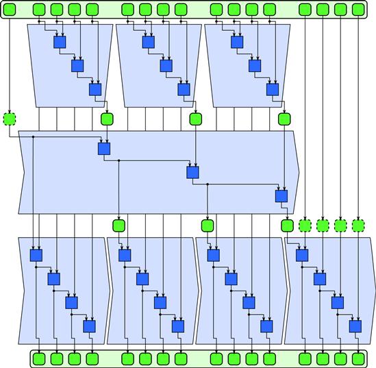
Figure 5.6 Three-phase tiled implementation of inclusive scan, including initial value.
Like many OpenMP programs, this code exploits knowing how many threads are available. The code attempts to use one tile per thread. Outside the parallel region the code computes how many threads to request. The clause num_threads(t) specifies this request. There is no guarantee that the full request will be granted, so inside the parallel region the code recomputes the tile size and number of tiles based on how many threads were granted. Our code would still be correct if it did not recompute these quantities, but it might have a load imbalance and therefore be slower, because some threads would execute more tiles than other threads.
Each phase waits for the previous phase to finish, but threads do not join between the phases. The first and last phases run with one thread per tile, which contributes Θ(N![]() P) to the asymptotic running time. The middle phase, marked with omp single, runs on a single thread. This phase contributes Θ(P) to the running time. During this phase, the other m threads just wait while this phase is running. Making threads wait like this is both good and bad. The advantage is that the threads are ready to go for the third phase, and the mapping from threads to tiles is preserved by the default scheduling of omp for loops. This minimizes memory traffic. The disadvantage is that the worker threads are committed when entering the parallel region. No additional workers can be added if they become available, and no committed workers can be removed until the parallel region completes.
P) to the asymptotic running time. The middle phase, marked with omp single, runs on a single thread. This phase contributes Θ(P) to the running time. During this phase, the other m threads just wait while this phase is running. Making threads wait like this is both good and bad. The advantage is that the threads are ready to go for the third phase, and the mapping from threads to tiles is preserved by the default scheduling of omp for loops. This minimizes memory traffic. The disadvantage is that the worker threads are committed when entering the parallel region. No additional workers can be added if they become available, and no committed workers can be removed until the parallel region completes.
5.5 Fusing Map and Scan
As with reduce, scan can be optimized by fusing it with adjacent operations.
Consider in particular the three-phase implementation of scan. Suppose such a scan is preceded by a map and followed by another map. Then, as long as the tiles are the same size, the tiles in the first map can be combined with the serial reductions in the first phase of the scan, and the tiled scan in the third phase can be combined with the following tiled map. This is shown in Figure 5.7. This creates more arithmetically intense code blocks and can cut down significantly on memory traffic and synchronization overhead.
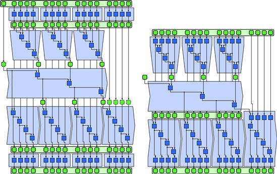
Figure 5.7 Optimization of map and three-phase scan by fusion. The initial and final phases of the scan can be combined with maps appearing in sequence before and after the scan. There is also an opportunity to fuse an initial map with the scan and final map of the last tile, but it is only a boundary case and may not always be worth doing.
It would also be possible to optimize a scan by fusing it with following reductions or three-phase scans since the first part of a three-phase scan is a tile reduction. However, if a reduction follows a scan, you can get rid of the reduction completely since it is available as an output of the scan, or it can be made available with very little extra computation.
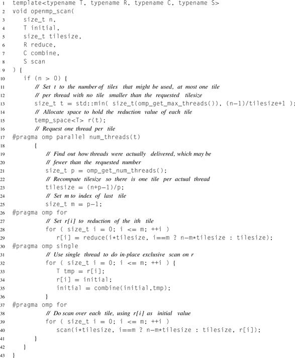
Listing 5.16 Three-phase tiled implementation of a scan in OpenMP. The interface is similar to the Cilk Plus implementation explained in Section 5.4, except that tilesize may be internally adjusted upward so that the number of tiles matches the number of threads. Listing 8.7 on page 227 has the code for template class temp_space.
5.6 Integration
Scan shows up in a variety of unexpected circumstances, and is often the key to parallelizing an “unparallelizable” algorithm. However, here we show a simple application: integrating a function. The scan of a tabulated function, sometimes known as the cumulation of that function, has several applications. Once we have computed it, we can approximate integrals over any interval in constant time. This can be used for fast, adjustable box filtering. A two-dimensional version of this can be used for antialiasing textures in computer graphics rendering, an approach known as summed area tables [Cro84].
One disadvantage of summed-area tables in practice, which we do not really consider here, is that extra precision is needed to make the original signal completely recoverable by differencing adjacent values. If this extra precision is not used, the filtering can be inaccurate. In particular, in the limit as the filter width becomes small we would like to recover the original signal.
As another important application, which we, however, do not discuss further in this book, you can compute random numbers with the distribution of a given probability density by computing the cumulation of the probability density distribution and inverting it. Mapping a uniform random number through this inverted function results in a random number with the desired probability distribution. Since the cumulation is always monotonic for positive functions, and probability distributions are always positive, this inversion can be done with a binary search. Sampling according to arbitrary probability density distributions can be important in Monte Carlo (random sampling) integration methods [KTB11].
5.6.1 Description of the Problem
Given a function f and interval [a, b], we would like to precompute a table that will allow rapid computation of the definite integral of f over any subinterval of [a, b]. Let ![]() . The table is a running sum of samples of f, scaled by Δx:
. The table is a running sum of samples of f, scaled by Δx:
![]()
The integral of f over [c, d] can be estimated by:
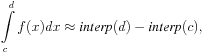
where interp(x) denotes linear interpolation on the table.
5.6.2 Serial Implementation
Listing 5.17 shows a serial implementation of the sampling and summation computation. It has a loop-carried dependence, as each iteration of the loop depends on the previous one.
Sometimes you will want to use a generic function defined in a function template as in Listing 5.18. To pass such a function as an argument, it is helpful to first instantiate it with particular types as in Listing 5.19.
Listing 5.20 shows how to compute the definite integral from two samples. It defines a helper function serial_sample that does linearly interpolated lookup on the array. Out of bounds subscripts are handled as if the original function is zero outside the bounds, which implies that the integral is zero to the left of the table values and equal to table[n−1] to the right of the table.
5.6.3 Cilk Plus
Listing 5.21 shows the Cilk Plus code for preparing the integration table. The initial mapping of the function is fused into the functor for doing tile reductions. The final scaling of the scan is fused in the functor for doing tile scans.
Scan is not a built-in operation in Cilk Plus, but we discuss its interface in Section 5.4 and its implementation in Section 8.11.
5.6.4 OpenMP
Listing 5.21 can be translated to OpenMP by making two changes:
• Replace cilk_scan with openmp_scan (Listing 5.16).
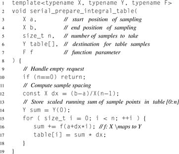
Listing 5.17 Serial integrated table preparation in C++. The code has a single loop that samples function f provided as an argument, performs an inclusive scan, and scales the results of the scan by dx.
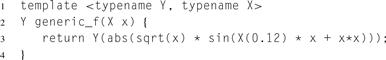
Listing 5.18 Generic test function for integration.
![]()
Listing 5.19 Concrete instantiation of test function for integration.
The second change is optional, since OpenMP plus Cilk Plus array notation can be an effective way to exploit both thread and vector parallelism. Of course, this requires a compiler that supports both.
Scan is not a built-in operation in OpenMP, but we discuss its implementation using a three-phase approach in Section 5.4.
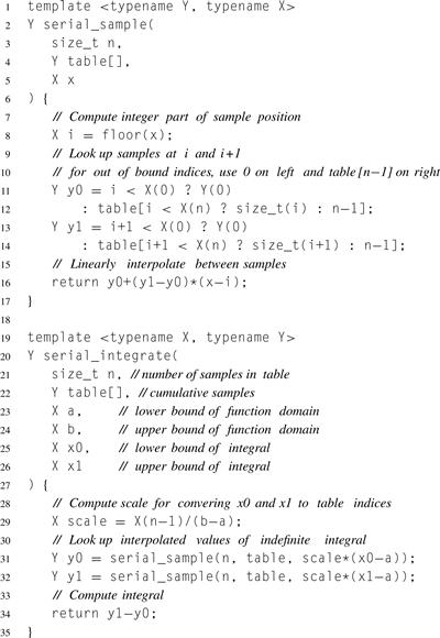
Listing 5.20 Serial implementation of integrated table lookup in C++. Two linearly interpolated samples of the table are taken and interpolated. Out-of-bounds indices are handled as if the original function (not the integral) is zero outside the bounds.
5.6.5 TBB
The TBB parallel_scan algorithm template has an internal optimization that lets it avoid calling the combiner function twice for each element when no actual parallelism occurs. Unfortunately, this optimization prevents fusing a map with the reduce portion of a scan. Consequently, the TBB implementation of the integration example must compute each sample point on both passes through a tile. The second pass has no easy way to know if the first pass occurred and, so there is no point in the first pass storing the samples. If the samples are expensive to compute, to avoid the extra computation we can precompute the samples and store them in a table before calling the scan. Here we assume the samples are relatively inexpensive to compute.
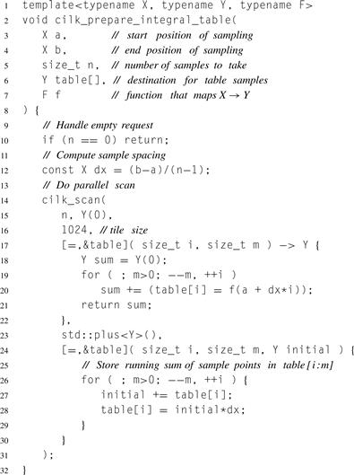
Listing 5.21 Integrated table preparation in Cilk Plus. The code implements the interface discussed in Section 5.4.
Listing 5.22 shows the code. In the TBB implementation a single templated operator() serves as both a both tiled reduce and a tiled scan. The idea behind this is that the code may have full or partial information about preceding iterations. The value of the expression tag.is_final_scan() distinguishes these two cases:
true: The state of the Body is the same as if all iterations of the loop preceding subrange r. In this case, operator() does a serial scan over the subrange. It leaves the Body in a state suitable for continuing beyond the current subrange.
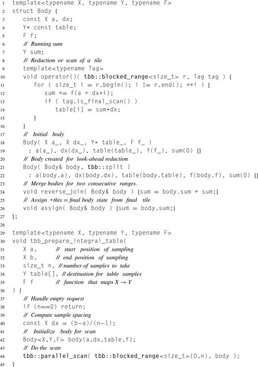
Listing 5.22 Integrated table preparation in TBB. Class Body defines all the significant actions required to do a scan.
false: The state of the Body represents the effect of zero or more consecutive iterations preceding subrange r, but not all preceding iterations. In this case, operator() updates the state to include reduction of the current subrange.
The second case occurs only if a thread actually steals work for the parallel_scan.
Method reverse_join merges two states of adjacent subranges. The “reverse” in its name comes from the fact that *this is the state of the right subrange, and its argument is the left subrange. The left subrange can be either a partial state or a full state remaining after a serial scan.
Method assign is used at the very end to update the original Body argument to tbb::parallel_scan with the Body state after the last iteration.
5.6.6 ArBB
Listing 5.23 shows the ArBB code for generating the table and Listing 5.24 shows the ArBB code for computing the integral by sampling this table.
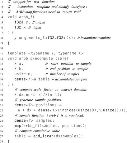
Listing 5.23 Integrated table preparation in ArBB. This simply invokes the built-in collective for inclusive scan using the addition operator. Templating the code provides generality.
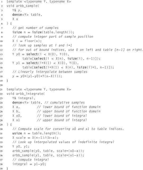
Listing 5.24 Integrated table lookup in ArBB. Two linearly interpolated samples of the table are taken and interpolated. Various other operations are required to avoid reading out of bounds on the arrays. This code is similar to the serial code, except for changes in types. The ? operator used in the serial code also has to be replaced with select. Unfortunately, the ? operator is not overloadable in ISO C++.
Listing 5.23 uses a special function to generate a set of integers. Vector arithmetic converts these integers into sample positions and then uses a map to generate all the samples. Finally, a scan function computes the cumulative table. The ArBB implementation will actually fuse all these operations together. In particular, the computation of sample positions, the sampling of the function, and the first phase of the scan will be combined into a single parallel operation.
Given the table, the integral can be computed using the function given in Listing 5.24. This function can be used to compute a single integral or an entire set if it is called from a map. This code is practically identical to the serial code in Listing 5.20. The templates take care of most of the type substitutions so the only difference is the use of an ArBB collection for the table.
5.7 Summary
This chapter discussed the collective reduce and scan patterns and various options for their implementation and gave some simple examples of their use. More detailed examples are provided in later chapters.
Generally speaking, if you use TBB or Cilk Plus, you will not have to concern yourself with many of the implementation details for reduce discussed in this chapter. These details have been introduced merely to make it clear why associative operations are needed in order to parallelize reduce and why commutativity is also often useful.
Scan is built into TBB and ArBB but not Cilk Plus or OpenMP. However, we provide an efficient implementation of scan in Cilk Plus in Section 8.11. This chapter also presented a simple three-phase implementation of scan in OpenMP, although this implementation is not as scalable as the one we will present later based on fork–join.
Reduce and scan are often found together with map, and they can be optimized by fusing their implementations or parts of their implementation with an adjacent map, or by reversing the order of map and reduce or scan. We discussed how to do this in TBB and Cilk Plus and provided several examples, whereas ArBB does it automatically.
1 This is also called “block,” but since that term can be confused with synchronization we avoid it here.
2 Proof: The arithmetic mean of two positive values is always greater than or equal to their geometic mean, and the means are equal only when the two values are equal. The geometric mean of N/P and P is ![]() , and their arithmetic mean is
, and their arithmetic mean is ![]() . Thus, the latter is minimized when N/P = P; that is,
. Thus, the latter is minimized when N/P = P; that is, ![]() .
.