
Chapter 8
Fork–Join
When you come to a fork in the road, take it.
(Yogi Berra, 1925-)
This chapter describes the fork–join pattern and gives several examples, including its use to implement other patterns such as map, reduce, recurrence, and scan. Applied recursively, fork–join can generate a high degree of potential parallelism. This can, in turn, be efficiently scheduled onto actual parallelism mechanisms by the Cilk Plus and Intel Threading Building Blocks (TBB) work-stealing schedulers.
Many serial divide-and-conquer algorithms lend themselves to parallelization via fork–join. However, the limits on speedup noted in Section 2.5 need to be taken into account. In particular, most of the work should be pushed as deep into the recursion as possible, where the parallelism is high.
This chapter starts with the basic concept of fork and join and introduces the Cilk Plus, TBB, and OpenMP syntaxes for it. Section 8.3 shows how the map pattern can be implemented efficiently using recursive fork–join, which is indeed how Cilk Plus and TBB implement it. Both Cilk Plus and TBB use a parallel iteration idiom for expressing the map pattern, although the TBB interface can also be thought of as using an elemental function syntax. The recursive approach to parallelism needs split and merge operations as well as a base case. Section 8.4 covers how to select the base case for parallel recursion. Section 8.5 explains how the work-stealing schedulers in Cilk Plus and TBB automatically balance load. It also details the subtle differences in work-stealing semantics between the two systems and the impact of this on program behavior—in particular, memory usage. Section 8.6 shows a common cookbook approach to analyzing the work and span of fork–join, particularly the recursive case. To demonstrate this approach and to give a concrete example of recursive parallelism, Section 8.7 presents an implementation of Karatsuba multiplication of polynomials. Section 8.8 touches on the subject of cache-oblivious algorithms. Cache-oblivious algorithms [ABF05] optimize for the memory hierarchy without knowing the structure or size of that hierarchy by having data locality at many different scales. Section 8.9 presents parallel Quicksort in detail, because it exposes subtle implementation issues that sometimes arise in writing efficient parallel divide-and-conquer algorithms. Parallel Quicksort also highlights the impact of the differences in Cilk Plus versus TBB work-stealing semantics. Section 8.10 shows how Cilk Plus hyperobjects can simplify writing reductions in the fork–join context. Section 8.11 shows how the scan pattern can be implemented efficiently with fork–join. Section 8.12 shows how fork–join can be applied to recurrences and, in particular, recursive tiled recurrences.
8.1 Definition
In fork–join parallelism, control flow forks (divides) into multiple flows that join (combine) later. After the fork, one flow turns into two separate flows. Each flow is independent, and they are not constrained to do similar computation. After the join, only one flow continues.
For example, consider forking to execute B() and C() in parallel and then joining afterwards. The execution of a fork–join can be pictured as a directed graph, as in Figure 8.1. This figure also demonstrates the graphical notation we will use for the fork and join operations.

Figure 8.1 Fork–join control flow.
Often fork–join is used to implement recursive divide-and-conquer algorithms. The typical pattern looks like this:
void DivideAndConquer( Problem P) {
if(P is base case) {
Solve P;
} else {
Divide P into K subproblems;
Fork to conquer each subproblem in parallel;
Join;
Combine subsolutions into final solution;
}
}
It is critical that the subproblems be independent, so that they can run in parallel. Nesting K-way fork–join this way to N levels permits KN-way parallelism. Figure 8.2 shows three-level nesting, resulting in eight parallel flows at the innermost level. The algorithm should be designed to put the vast majority of work deep in the nest, where parallelism is high. Section 8.6 shows how to formally analyze the speedup of fork–join.
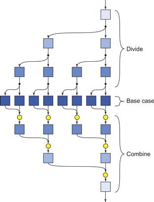
Figure 8.2 Nested fork–join control flow in a divide-and-conquer algorithm. For good speedup, it is important that most of the work occur deep in the nesting (more darkly shaded boxes), where parallelism is high.
Selecting the size of the base case for parallel divide-and-conquer can be critical in practice. It should allow the recursion to go deep enough to permit plenty of parallelism. However, the recursion should not be too deep; in particular, it should not result in subproblems so fine grained that scheduling overheads dominate. Section 8.4 offers more guidance on this point. Also, the problem division and combine operations which appear before and after the fork and join operations should be as fast as possible, so they do not dominate the asymptotic complexity and strangle speedup.
8.2 Programming Model Support for Fork–Join
Programming model support for fork–join has to express where to fork and where to join. Cilk Plus, TBB, and OpenMP express fork–join differently. Cilk Plus uses a syntactic extension, TBB uses a library, and OpenMP uses pragma markup, but the fundamental parallel control flow is the same for all. There are, however, subtle differences about which threads execute a particular part of the parallel control flow, as Section 8.5 will explain. As long as you do not rely on thread-local storage, the difference is immaterial for now.
When reading the following subsections, pay attention not only to the different ways of expressing fork–join but also to how variables outside the fork–join are captured and referenced. This is particularly relevant when there is an increment of an index variable, such as ++i in the example.
8.2.1 Cilk Plus Support for Fork–Join
Cilk Plus has keywords for marking fork and join points in a program. The control flow in Figure 8.1 can be written in Cilk Plus as:
cilk_spawn B();
C();
cilk_sync;
The cilk_spawn marks the fork. It indicates that the caller can continue asynchronously without waiting for B() to return. The precise fork point occurs after evaluation of any actual arguments. The cilk_sync marks an explicit join operation. It indicates that execution must wait until all calls spawned up to that point by the current function have returned. In Cilk Plus there is also an explicit join at the end of every function.
Note in our example above that there is not a cilk_spawn before C(). The example could also be written as the following, which would work:
cilk_spawn B();
cilk_spawn C();
/* nil */
cilk_sync;
However, this is redundant and considered bad style in Cilk Plus, because it specifies two forks, as in Figure 8.3. The second fork is pointless overhead—it runs /* nil */ (that is, nothing) in the spawning task in parallel with C(). You should put some of the work in the spawned task and some in the spawning task instead.
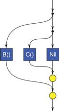
Figure 8.3 Bad style for fork–join. Spawning every subtask in Cilk Plus is unnecessary overhead. In general, work should also be computed by the spawning task.
Multiway forks are possible. For example, the following code forks four ways:
cilk_spawn A();
cilk_spawn B();
cilk_spawn C();
D(); //Not spawned, executed in spawning task
cilk_sync; //Join
The matching of cilk_spawn and cilk_sync is dynamic, not lexical. A cilk_sync waits for all spawned calls in the current function to return. Spawning within a loop, or conditional spawning, can be handy on occasion. The following fragment does both: It spawns f(a[i]) for nonzero a[i]:
for (int i=0; i<n; ++i)
if (a[i]!=0)
cilk_spawn f(a[i]);
cilk_sync;
Be warned, however, that spawning many tasks from a loop is often less efficient than using recursive forking, because the loop itself may become a serial bottleneck. The cilk_for construct uses recursive forking even though it looks like a loop. The cilk_sync can be conditional, too, although none of the examples in this book uses that capability. As mentioned previously, there is always an implicit cilk_sync (join) at the end of a function. Therefore, when a function returns, you can be sure that any Cilk Plus parallelism created in it has finished. Note, too, that because forking occurs after evaluation of any actual arguments, each spawned call receives the intended value of a[i] as an argument, even as the loop continues to increment i.
8.2.2 TBB Support for Fork–Join
TBB has two high-level algorithm templates for fork–join, one for simple cases and one for more complicated cases. For simple cases, the function template parallel_invoke does an n-way fork for small n. It also waits for all tasks that it forks to complete; that is, it joins all the tasks before returning. Here is an example for n = 2:
tbb::parallel_invoke(B, C);
In the current TBB implementation, the parallel_invoke template accepts up to 10 arguments.
The arguments should be function objects, sometimes called functors, each with a method void operator()()const that takes no arguments. Passing parameters to the functor is done by capturing them during construction. Typically the function objects are constructed by lambda expressions, which give a more convenient syntax, especially for capturing parameters. For example, here is a hypothetical fragment for walking two subtrees in parallel:
tbb::parallel_invoke([=]{Walk(node->left);},
[=]{Walk(node->right);});
The class tbb::task_group deals with more complicated cases, and in particular provides a more explicit join operation. Here is a TBB fragment for spawning f(a[i]) for nonzero a[i]:
task_group g;
for (int i=0; i<n; ++i)
if (a[i] != 0)
g.run([=,&a]f(a[i]);); // Spawn f(a[i]) as child task
g.wait(); // Wait for all tasks spawned from g
Method run marks where a fork occurs; method wait marks a join. The wait is required before destroying the task_group; otherwise, the destructor throws an exception missing_wait. Note that i must be captured by value, not by reference, because the loop might increment the original variable i before the functor actually runs. By-value capture makes a copy of non-local variable references at the point where the lambda is constructed. By-reference allows the lambda to refer to the state of the non-local variable when the lambda is actually executed. More details on this are given in Section D.2. The general by-value capture given by the “=” argument to the lambda ensures that the value of i at the point of the invocation of g.run is used for that task. The notation &a specifies that a is captured by reference, since C++ does not allow capturing arrays by value.
8.2.3 OpenMP Support for Fork–Join
OpenMP 3.0 also has a fork–join construct. Here is an OpenMP fragment for the fork–join control flow from Figure 8.1:
#pragma omp task
B();
C();
#pragma omp taskwait
The construct task indicates that the subsequent statement can be independently scheduled as a task. In the example, the statement “B();” is run in parallel. The statement could also be a compound statement—that is, a group of statements surrounded by braces. The work in C() is performed by the spawning task, and finally the construct omp taskwait waits for all child tasks of the current task.
There is a catch peculiar to OpenMP: Parallelism happens only inside parallel regions. Thus, for the example to actually fork there must be an enclosing OpenMP parallel construct, either in the current routine or further up the call chain.
Variable capture needs attention. OpenMP tasks essentially capture global variables by reference and local variables by value. In OpenMP parlance, these capture modes are respectively called shared and firstprivate. Sometimes these defaults must be overridden, as the following fragment illustrates:
int foo(int i) {
int x, y;
#pragma omp task shared(x)
x = f(i);
++i;
y = g(i);
#pragma omp taskwait
return x+y;
}
The shared clause requests that x be captured by reference. Without it, x would be captured by value, and the effect of the assignment x = f(i) would be lost.
8.3 Recursive Implementation of Map
One of the simplest, but most useful, patterns to implement with fork–join is map. Although both Intel TBB and Cilk Plus have concise ways to express map directly, the map pattern is nonetheless a good starting example for parallel divide-and-conquer, because it implements a familiar pattern. It also gives some insight into how Cilk Plus and TBB implement their map constructs. They really do use the divide-and-conquer approach to be described, because it efficiently exploits the underlying work-stealing mechanism explained in Section 8.5. Furthermore, you may eventually need to write a version of the map pattern with features beyond the built-in capabilities—for example, when fusing it with other patterns—so knowledge of how to implement map efficiently using fork–join is useful.
Consider the following Cilk Plus code:
cilk_for(unsigned i=lower; i<upper; ++i)
f(i);
The cilk_for construct can be implemented by a divide-and-conquer routine recursive_map, which is called like this:
if(lower<upper)
recursive_map(lower,upper,grainsize,f)
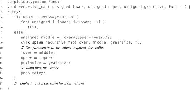
The conditional eliminates needing to deal with the empty case inside the routine. Listing 8.1 shows the recursive_map routine. The parameter grainsize controls the size of the base case. In Cilk Plus, the compiler and runtime choose the size of the base case based on considerations that will be discussed in Section 8.4.
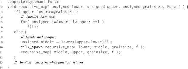
Listing 8.1 Recursive implementation of the map pattern in Cilk Plus.
Figure 8.4 illustrates the execution of recursive_map(0,9,2,f), which maps f over the half-open interval [0,9) with no more than two iterations per grain. Arcs are labeled with [lower,upper) to indicate the corresponding arguments to recursive_map.
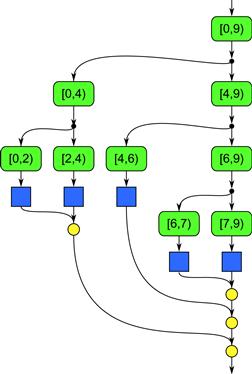
Figure 8.4 Execution of recursive_map(0,9,2,f) using the implemention in Listing 8.1.
Now consider an optimization. In Listing 8.1, no explicit cilk_sync is necessary because every function with cilk_spawn performs an implicit cilk_sync when it returns. Except for this implicit cilk_sync, the routine does nothing after its last call. Hence, the last call is what is known as a tail call. In serial programming, as long as local variables can be overwritten before the last call, a tail call can be optimized away by the following transformation:
Applying these rules literally to the previous example yields the code in Listing 8.2. This code can be cleaned up by removing redundant updates and structuring the goto as a while loop, resulting in the concise code in Listing 8.3.
Similar tricks for converting tail calls to iteration applies to TBB, as will be shown in Listings 8.12 and 8.13 of Section 8.9.2.
Listing 8.2 Modification of Listing 8.1 that changes tail call into a goto.
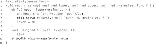
Listing 8.3 Cleaned-up semi-recursive map in Cilk Plus.
8.4 Choosing Base Cases
In parallel divide-and-conquer, there are often two distinct base cases to consider:
They sometimes differ because they are guided by slightly different overhead considerations. The alternative to parallel recursion is serial recursion, which avoids parallel scheduling overheads. The alternative to serial recursion is a serial iterative algorithm, which avoids calling overheads. However, these two overheads are often at different scales so the optimal sizes for the base cases are often different.
For example, in the Quicksort example detailed later in Section 8.9, serial recursion continues only until there are about 7 elements to sort. It stops at a relatively short sequence because the iterative alternative is a quadratic sort, which has a higher asymptotic complexity but less overhead and a lower constant factor. However, in the same example, parallel recursion stops at about 500 elements. The parallel recursion stops for a much bigger base case problem size because the alternative is serial recursive Quicksort, which is still quite efficient at this size but avoids parallel overheads.
Given a machine with P hardware threads, it is tempting to choose a parallel base case such that there are exactly P leaves in the tree of spawned functions. However, doing so often results in poor performance, because it gives the scheduler no flexibility to balance load, as noted in Section 2.6.6. Even if the leaves have nominally equal work and processors are nominally equivalent, system effects such as page faults, cache misses, and interrupts can destroy the balance. Thus, it is usually best to overdecompose the problem to create parallel slack (Section 2.5.6). As the next section explains, the underlying work-stealing scheduler in Cilk Plus and TBB makes unused parallel slack cheap for fork–join parallelism.
Of course, overdecomposition can go too far, causing scheduling overheads to swamp useful work, just as ordinary function calls can swamp useful work in serial programs. A rough rule of thumb is that a cilk_spawn costs on the order of 10 non-inlined function calls, and a TBB spawn costs on the order of 30 non-inlined function calls, excluding the cost of data transfer between workers if parallelism actually occurs. Basic intuitions for amortizing call overhead still apply—only the relative expense of the call has changed.
When the leaves dominate the work, you should also consider whether vector parallelism can be applied, as in the Karatsuba multiplication example (Listing 8.6).
8.5 Load Balancing
Cilk Plus and TBB efficiently balance the load for fork–join automatically, using a technique called work stealing. Indeed, as remarked earlier, the work-stealing technique is so effective for load balancing that both frameworks implement their map operations (cilk_for and tbb::parallel_for) using fork–join algorithms.
In a basic work-stealing scheduler, each thread is called a worker. Each worker maintains its own double-ended queue (deque) of tasks. Call one end of the deque the “top” and the other end the “bottom.” A worker treats its own deque like a stack. When a worker spawns a new task, it pushes that task onto the top of its own deque. When a worker finishes its current task, it pops a task from the top of its own deque, unless the deque is empty.
When a worker’s deque is empty, a worker chooses a random victim’s deque and steals a task from the bottom of that deque. Because that is the last task that the owner of the deque would touch, this approach has several benefits:
• The thief will be grabbing work toward the beginning of the call tree. This tends to be a big piece of work that will keep the thief busy longer than a small piece would.
• In the case of recursive decomposition of an index space, the work stolen will have indices that are consecutive but will tend to be distant from those that the victim is working on. This tends to avoid cache conflicts when iterating over arrays.
Overall, the net effect is that workers operate serially depth-first by default, until more actual parallelism is required. Each steal adds a bit of parallel breadth-first execution, just enough to keep the workers busy. The “just enough” part is important. Always doing breadth-first execution leads to space exponential in the spawning depth, and the worst spatial locality imaginable! Cilk Plus formalizes the “just enough” notion into some strong guarantees about time and space behavior.
Before going into the Cilk Plus guarantees, it is worth understanding why they will not always apply to TBB also. Cilk Plus and TBB differ in their concept of what is a stealable task. The code fragments in Listing 8.4 will be used to show the difference. The Cilk Plus and TBB fragments show poor style, because the code will probably perform much better if written as a map instead of a serial loop that creates tasks. But it serves well to illustrate the stealing issue, and sometimes similar code has to be written when access to the iteration space is inherently sequential, such as when a loop traverses a linked list.
For each spawned f(i), there are two conceptual tasks:
• Continuation of executing the caller. This task, which has no name, is naturally called a continuation.
A key difference between Cilk Plus and TBB is that in Cilk Plus, thieves steal continuations. In TBB, thieves steal children.
Figure 8.5 diagrams the difference, assuming there are plenty of workers to steal work. The left side shows Cilk Plus execution, which uses steal-continuation semantics. The initial worker sets i=0 and spawns f(0). The worker immediately starts executing f(0), leaving the continuation available to steal. Then another worker steals that continuation and continues execution of the loop. It updates i and executes f(1). The next worker steals the further continuation of the loop and executes f(2). The key point is that the loop advances only when there is a worker ready to execute another iteration of it.
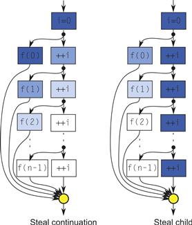
Figure 8.5 Steal continuation vs. steal child. The diagrams show the execution of the routines in Listing 8.4. Each task is shaded according to which worker executes it if there are plenty of workers. In steal-continuation semantics, a thief steals the continuation, and the original worker executes the child. Steal-child semantics are the other way around.
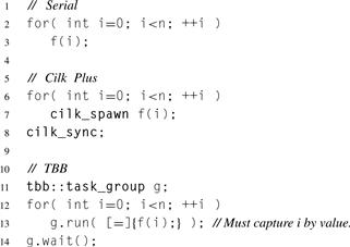
Listing 8.4 Three loop forms illustrating steal-continuation versus steal-child semantics for work-stealing. This is generally a poor way to parallelize a loop but is useful for discussing differences in stealing. Note that the TBB code needs to capture i by value, before the next ++i happens.
The right side shows TBB execution, which uses steal-child semantics. The initial worker sets i=0 and spawns f(0). It leaves f(0) available to steal and proceeds to go around the loop again. It thus executes all iterations of the loop before attending to spawned work. Furthermore, if it does pick up an iteration afterward, f(n-1) is topmost on its deque, so it executes f(n-1) first, the reverse order of the serial code.
This difference has a major impact on stack space guarantees. In the Cilk Plus execution, each worker is working on a call chain in a state that would have existed in the serial program. Thus, Cilk Plus can guarantee that, if a program takes stack space ![]() for serial execution, it takes no more than stack space
for serial execution, it takes no more than stack space ![]() when executed by P workers.1 However, if run with a single worker, the TBB code creates a state where the for loop completes, but none of the calls to f(i) has yet started, a nonsensical state for the original program. Assuming each spawned call takes Θ (1) space to represent on the stack, the TBB program takes Θ (n) stack space, even if no parallelism is being exploited.
when executed by P workers.1 However, if run with a single worker, the TBB code creates a state where the for loop completes, but none of the calls to f(i) has yet started, a nonsensical state for the original program. Assuming each spawned call takes Θ (1) space to represent on the stack, the TBB program takes Θ (n) stack space, even if no parallelism is being exploited.
The example also illustrates another difference. In the TBB code, the worker that enters the loop is the worker that continutes execution after f(i) finishes. If that worker executes g.wait() and not all f(i) are finished, it tries to execute some of the outstanding f(i) tasks. If none of those is available, it either idly waits or goes off on an errand to find temporary work to keep it busy. If, in the meantime, the other spawned f(i) finishes, further progress is blocked until the original worker returns from its errand. Thus, TBB scheduling is not always greedy (Section 2.5.6), which in turn means that, strictly speaking, the lower bound on speedup derived in Chapter 2 does not apply.
In the Cilk Plus code, workers never wait at a cilk_sync. The last worker to reach the cilk_sync is the worker that continues execution afterwards. Any worker that reaches the cilk_sync earlier abandons the computation entirely and tries to randomly steal work elsewhere. Though random stealing deviates from ideal greediness, in practice as long as there is plenty of parallel slack the deviation is insignificant and Cilk Plus achieves the time bound in Equation 2.9 (page 64).
TBB can implement steal-continuation semantics, and achieve the Cilk Plus space and time guarantees, if continuations are represented as explicit task objects. This is called continuation passing style. Unfortunately, it requires some tricky coding, as Section 8.9.2 will show.
Cilk Plus and TBB have different semantics because they are designed with different tradeoffs in mind. Cilk Plus has nicer properties but requires special compiler support to deal with stealing continuations, and it is limited to a strict fork–join model. TBB is designed as a plain library that can be run by any C++ compiler and supports a less strictly structured model.
The stealing semantics for OpenMP are complex and implementation dependent. The OpenMP rules [Boa11] imply that steal-child must be the default but permits steal-continuation if a task is annotated with an untied clause. However, the rules do not require continuation stealing, so the benefits of these semantics are not guaranteed even for untied tasks in OpenMP.
8.6 Complexity of Parallel Divide-and-Conquer
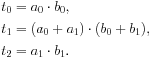
Computing the work and span of the basic fork–join pattern is straightforward. Suppose execution forks along multiple paths and rejoins. The total work T1 is the sum of the work along each path. The span T∞ is the maximum span of any path.
More formally, let ![]() denote the fork–join composition of B and C, as introduced earlier in Figure 8.1. The overall work and span are:
denote the fork–join composition of B and C, as introduced earlier in Figure 8.1. The overall work and span are:
![]()
Realistically, there will be some overhead for forking and joining. The burdened span (see Section 2.5.6) includes this overhead, typically a small constant addition for the synchronization plus the cost of communicating cache lines between hardware threads.
Since parallel divide-and-conquer is a recursive application of fork–join composition, analyzing the work and span in a recursive divide-and-conquer algorithm is a matter of defining recurrence relations for T1 and T∞ and solving them. Typically, the recurrences for T1 and T∞ have similar form but differ in constant factors, which can cause them to have quite different asymptotic solutions. Though solving arbitrary recurrence relations can be difficult, the relations for divide-and-conquer programs often have a form for which a closed-form solution is already known.
The following discussion presents a simplified form of the Master method [CLRS09], which suffices for the most common cases. It assumes that the problem to be solved has a size N and the recursion has these properties:
• The recursion step solves a subproblems, each of size N/b.
Here time means either T1 or T∞, depending on context, so to explain the generic math an unadorned T will be used.
Let T (N) denote the time required to execute a divide-and-conquer algorithm with the aforementioned properties. The recurrence relations will be:
![]()
There are three asymptotic solutions to this recurrence:
![]() 8.1
8.1
![]() 8.2
8.2
![]() 8.3
8.3
None of the solutions mentions c or e directly—those are scale factors that disappear in the Θ notation. What is important is the value of logba relative to d.
The intuition behind these solutions is as follows. A full proof is given in Cormen et al. [CLRS09]. Start by partitioning the program’s recursive call tree level by level, with the levels labeled, from top to bottom, as N, N/b, N/b2, N/b3, and so on. The three cases in the solution correspond to which levels dominate the work. Let r be the work at level N/b divided by the work at level N. Each problem has a subproblems that are proportionately smaller by 1/b. Each problem will require cNd work itself and have a children requiring c(N/b)d work on the next level down. So, ![]() . Three distinct cases arise, as illustrated in the diagrams in Figure 8.6 for some specific values of a and b, with c = d = e = 1. The general cases and their corresponding illustrations are:
. Three distinct cases arise, as illustrated in the diagrams in Figure 8.6 for some specific values of a and b, with c = d = e = 1. The general cases and their corresponding illustrations are:
Case 1. If ![]() , then
, then ![]() . The work at each level exponentially increases with depth, so levels near the bottom dominate.
. The work at each level exponentially increases with depth, so levels near the bottom dominate.
Case 2. If ![]() , then r = 1. The work at each level is about the same, so the work is proportional to the work at the top level times the number of levels.
, then r = 1. The work at each level is about the same, so the work is proportional to the work at the top level times the number of levels.
Case 3. If ![]() , then
, then ![]() . The work at each level exponentially decreases with depth. So levels near the top dominate.
. The work at each level exponentially decreases with depth. So levels near the top dominate.
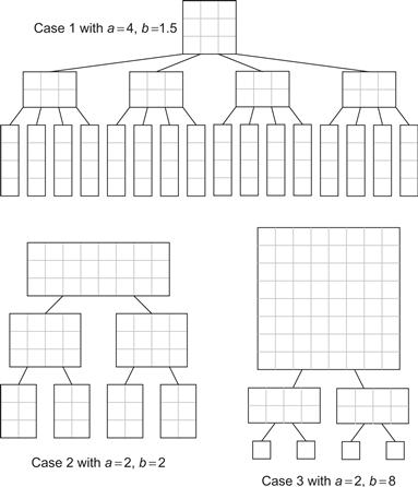
Figure 8.6 The three cases in the Master method. Each grid square represents a unit of work.
A useful intuition for effective parallelization can be drawn from these general notions. Ideally, the subproblems are independent and can be computed in parallel, so only one of the subproblems contributes to T∞. So a = 1 in the recurrences for T∞, and consequently ![]() . Since
. Since ![]() for any real program, only two of the closed-form solutions apply to T∞:
for any real program, only two of the closed-form solutions apply to T∞:
![]()
Thus, for divide-and-conquer algorithms that fit our assumptions, T∞ can be logarithmic at best, and only if the divide and combine steps take constant time.
Sometimes, as for the Merge Sort in Chapter 13, constant-time divide and combine is not practical, but logarithmic time is. The recurrences for such algorithms replace the cNd term with a more complicated term and are beyond the scope of this discussion. See Cormen et al. [CLRS09] for a more general form of the recurrences and their closed-form solution, and Akra and Bazzi [AB98] for an even more general form.
8.7 Karatsuba Multiplication of Polynomials
Polynomial multiplication serves as an example of applying the the Master method to real code. Before delving into the fork–join algorithm and its analysis, let’s consider the basic flat algorithm for multiplying polynomials A and B, each with n coefficients. The flat algorithm is essentially grade-school multiplication, except no carries propagate between terms. Listing 8.5 shows the flat algorithm implemented with Cilk Plus array notation.
Input arrays a and b each hold n coefficients of polynomials A and B, respectively. Output array c holds the ![]() coefficients of the output polynomial C.
coefficients of the output polynomial C.
The flat algorithm is concise and highly parallel for large n, but unfortunately creates Θ(n2) work. Karatsuba’s multiplication algorithm is a fork–join alternative that creates much less work. A slightly different form of it is sometimes used for multiplying numbers with hundreds of digits. Both forms are based on the observation that ![]() can be expanded to
can be expanded to ![]() using only three multiplications:
using only three multiplications:
The final expansion can be calculated as ![]() . Each of the three multiplications can be done by recursive application of Karatsuba’s method. The recursion continues until the multiplications become so small that the flat algorithm is more efficient.
. Each of the three multiplications can be done by recursive application of Karatsuba’s method. The recursion continues until the multiplications become so small that the flat algorithm is more efficient.
The interpretation of K depends on the meaning of multiplication:
• For convolution, K is a shift.
• For multiplication of polynomials in x, K is a power of x.
• For multiplication of numerals, K is a power of the radix.
For example, to do the radix 10 multiplication problem 1234 ⋅ 5678, K is initially 100, so the problem can be written as ![]() . The three requisite multiplications are:
. The three requisite multiplications are:
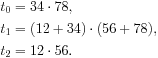
Each of these can be done via Karatsuba’s method with K = 10. Carry propagation can be deferred to the very end or done on the fly using carry-save addition.
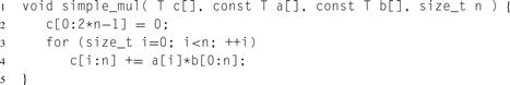
Listing 8.5 Flat algorithm for polynomial multiplication using Cilk Plus array notation.
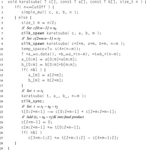
Listing 8.6 Karatsuba multiplication in Cilk Plus.
Listing 8.6 shows Cilk Plus code for Karatsuba multiplication. Translation to TBB is a matter of using task_group instead of cilk_spawn/cilk_sync, and it is possible to translate this code to OpenMP using tasking constructs.
The parameters are similar to those in Listing 8.5. The type temp_space, described in more detail in Section 8.7.1, holds scratch space for computing ![]() . The statements conditional on n&1 do a little extra work required for odd-length sequences and can be ignored to get the general idea of the algorithm.
. The statements conditional on n&1 do a little extra work required for odd-length sequences and can be ignored to get the general idea of the algorithm.
A coding point worth mentioning is that ![]() is computed separately before adjusting the final product in c. The reason why is that t0 and t2 are stored in array c. It would be incorrect to merge lines 22 and 25 into a single line like this:
is computed separately before adjusting the final product in c. The reason why is that t0 and t2 are stored in array c. It would be incorrect to merge lines 22 and 25 into a single line like this:
c[m:2∗m-1] += t[0:2∗m-1] - c[0:2∗m-1] - c[2∗m:2∗ m-1]; // Wrong!
because then there would be partial overlap of the source and destination array sections. No overlap or exact overlap is okay, but partial overlap causes undefined behavior as explained in Section B.8.5. Line 27 avoids the partial overlap issue because ![]() ; thus, the array sections c[3∗m-1:2] and c[4∗m-1:2] never overlap.
; thus, the array sections c[3∗m-1:2] and c[4∗m-1:2] never overlap.
To use the code for n-digit integer multiplication, make T an integral type large enough to hold n products of digits. Do the convolution, and then normalize the resulting numeral by propagating carries.
The extra work for when N is odd is insignificant, so assume N is even. Serial execution recurses on three half-sized instances. The additions and subtractions take time linear in N. The relations for T1 are:
![]()
This is case 1 in the Master method. Plugging in the closed-form solution yields:
![]()
The recurrence relations for T∞ differ in the coefficient. There are three subproblems being solved in parallel. Since they are all similar, T∞ is as if two of the subproblems disappeared, because their execution overlaps solution of the other subproblem. So the recurrence is:
![]()
This is case 3, with solution ![]()
The speedup limit is ![]() , so the speedup limit grows a little faster than
, so the speedup limit grows a little faster than ![]() .
.
The formulae also enable a ballpark estimate for a good parallel base case. We want the base case to have at least 1000 operations for Cilk Plus. Since the operation count grows as ![]() , that indicates that n = 100 is the right order of magnitude for the parallel base case.
, that indicates that n = 100 is the right order of magnitude for the parallel base case.
The space complexity of Karatsuba multiplication can also be derived from recurrences. Let ![]() be the space for serial execution. The recurrence for
be the space for serial execution. The recurrence for ![]() is
is
![]()
This is case 3, with solution ![]() .
.
Finally, consider ![]() , the space required if an infinite number of threads were available:
, the space required if an infinite number of threads were available:
![]()
which has the solution ![]() . Though a machine with an infinite number of threads is theoretical, there is a real, practical lesson here: Parallelizing divide-and-conquer by creating a new thread for each spawn can result in an exponential space explosion. Fortunately, there is a better way. As Section 8.5 shows, Cilk Plus work-stealing guarantees that
. Though a machine with an infinite number of threads is theoretical, there is a real, practical lesson here: Parallelizing divide-and-conquer by creating a new thread for each spawn can result in an exponential space explosion. Fortunately, there is a better way. As Section 8.5 shows, Cilk Plus work-stealing guarantees that ![]() , which enables Karatsuba multiplication to run in space
, which enables Karatsuba multiplication to run in space ![]() , much better than exponential space.
, much better than exponential space.
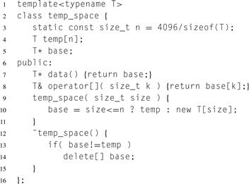
Listing 8.7 Type for scratch space. It is optimized for allocating short arrays of a type T with a trivial constructor and destructor.
8.7.1 Note on Allocating Scratch Space
The Karatsuba multiplication algorithm in Listing 8.6 could use a std::vector<T> for scratch space. But that would introduce the overhead of dynamic memory allocation even for relatively short arrays near the leaves of the computation, which dominate the execution time. Hence, the code uses the class temp_space shown in Listing 8.7 for scratch space.
For simplicity, this class always allocates n elements in temp and hence is suboptimal if type T has a non-trivial constructor or destructor. More complex implementations can remove this overhead.
At the time of this writing, C99 variable-length arrays or alloca cannot be used in a function that has cilk_spawn. The reason why is because these features allocate space on the current stack. The continuation after a cilk_spawn may be run on a stack different from the original stack of the caller, and this new stack disappears after a cilk_sync. Hence, anything allocated on that stack would be unsafe to access after the cilk_sync.
8.8 Cache Locality and Cache-Oblivious Algorithms
Although work and span analysis often illuminates fundamental limits on speedup, it ignores memory bandwidth constraints that often limit speedup. When memory bandwidth is the critical resource, it is important to reuse data from cache as much as possible instead of fetching it from main memory. Because the size of caches and the number of levels of cache vary between platforms, tailoring algorithms to cache properties can be complicated. A solution is a technique called cache-oblivious programming. It is really cache-paranoid programming because the code is written to work reasonably well regardless of the actual structure of the cache. In practice, there are possibly multiple levels of cache, and when you write the code you are oblivious to their actual structure and size.
Optimizing for an unknown cache configuration sounds impossible at first. The trick is to apply recursive divide-and-conquer, resulting in good data locality at multiple scales. As a problem is chopped into finer and finer pieces, eventually a piece fits into outer-level cache. With further subdivision, pieces may fit into a smaller and faster cache.
An example of cache-oblivious programming is dense matrix multiplication. The obvious non-recursive code for such multiplication uses three nested loops. Although choosing the right loop order can help somewhat, for sufficiently large matrices the three-loop approach will suffer when the matrices do not fit in cache. The cache-oblivious algorithm divides a matrix multiplication into smaller matrix multiplications, until at some point the matrices fit in cache. Better yet, the divide-and-conquer structure gives us an obvious place to insert fork–join parallelism.
Assume that A, B, and C are matrices, and we want to compute ![]() . A divide-and-conquer strategy is:
. A divide-and-conquer strategy is:
• If the matrices are small, use serial matrix multiplication.
• If the matrices are large, divide into two matrix multiplication problems.
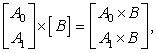
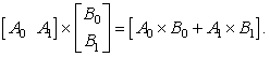
There are three ways to do the division, based on the following three identities:
![]() 8.4
8.4
 8.5
8.5
 8.6
8.6
Choosing the identity that splits the longest axis is a good choice, because then the submatrices will tend toward being square. That tends to maximize cache locality during multiplication.2
To see this, suppose A has dimensions m × k, and B has dimensions k × n. The total work T1 to multiply the matrices is O (m n k). The total space S to hold all three matrices is ![]() . This sum is minimal for a given product m n k when m = n = k. Hence, striving to make the matrices square improves the chance that the result fits within some level of cache.
. This sum is minimal for a given product m n k when m = n = k. Hence, striving to make the matrices square improves the chance that the result fits within some level of cache.
Listing 8.8 shows a pseudocode implementation. The informal notations rows(X) and cols(X) denote the number of rows and columns, respectively, of a matrix X. The first two recursive pairs of calls do parallel fork–join. They can be written in TBB using tbb::parallel_invoke. They are safe to execute in parallel because they update separate parts of matrix C. But the last recursive pair cannot execute in parallel, because both calls update the same matrix.
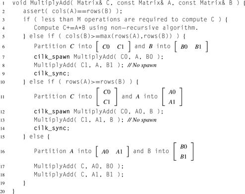
Listing 8.8 Pseudocode for recursive matrix multiplication.
Since the last case is serial and equivalent to a single MultiplyAdd, it is tempting to write MultiplyAdd in a way that uses only the first two of our splitting identities. Doing so would not affect the parallelism but could seriously raise consumption of memory bandwidth. To see this, consider what would happen in the base case: A and B would be very skinny, with A wide and B tall. In extreme, A would be an m-element column matrix and B would be an n-element row matrix. Their product would be an m × n matrix, requiring one store to memory for each multiplication.
The asymptotic complexity is:
![]() 8.7
8.7
For practical purposes, rows(B) is usually much larger than either of the lg factors, so the speedup limit is ![]() ; that is, the speedup is proportional to the size of the output matrix. To see this directly from the code, observe that the code is essentially doing a fork–join recursion over the output matrix and computing inner products for each output element. Thus, it is asymptotically equivalent to computing each element of C in parallel. But writing the code to directly do that would result in poor cache behavior, because each inner product would be consuming an entire row of A and column of B at once.
; that is, the speedup is proportional to the size of the output matrix. To see this directly from the code, observe that the code is essentially doing a fork–join recursion over the output matrix and computing inner products for each output element. Thus, it is asymptotically equivalent to computing each element of C in parallel. But writing the code to directly do that would result in poor cache behavior, because each inner product would be consuming an entire row of A and column of B at once.
It is possible to raise the speedup limit by using temporary storage, so that the serial pair of recursive calls can run in parallel, like this:
Matrix tmp = [0];
cilk_spawn MultiplyAdd(C, A0, B0);
MultiplyAdd(tmp, A1, B1); // No spawn
C += tmp;
Then ![]() , which is significantly lower than the bound in Equation 8.7. However, in practice the extra operations and memory bandwidth consumed by the final += make it a losing strategy in typical cases, particularly if the other fork–join parts introduce sufficient parallelism to keep the machine busy. In particular, the extra storage is significant. For example, suppose the top-level matrices A and B are square N × N matrices. The temporary is allocated every time the inner dimension splits. So the recurrences for the serial execution space S are:
, which is significantly lower than the bound in Equation 8.7. However, in practice the extra operations and memory bandwidth consumed by the final += make it a losing strategy in typical cases, particularly if the other fork–join parts introduce sufficient parallelism to keep the machine busy. In particular, the extra storage is significant. For example, suppose the top-level matrices A and B are square N × N matrices. The temporary is allocated every time the inner dimension splits. So the recurrences for the serial execution space S are:
![]()
which has the solution:
![]()
Since Cilk Plus guarantees that ![]() , the space is at worst
, the space is at worst ![]() . That is far worse than the other algorithm, which needs no temporary matrices and thus requires only
. That is far worse than the other algorithm, which needs no temporary matrices and thus requires only ![]() space.
space.
There are other recursive approaches to matrix multiplication that reduce T1 at the expense of complexity or space. For example, Strassen’s method [Str69] recurses by dividing A, B, and C each into quadrants and uses identities similar in spirit to Karatsuba multiplication, such that only 7 quadrant multiplications are required, instead of the obvious 8. Strassen’s algorithm runs in ![]() for multiplying
for multiplying ![]() matrices, and the quadrant multiplications can be computed in parallel.
matrices, and the quadrant multiplications can be computed in parallel.
8.9 Quicksort
Quicksort is a good example for studying how to parallelize a non-trivial divide-and-conquer algorithm. In its simplest form, it is naturally expressed as a recursive fork–join algorithm. More sophisticated variants are only partially recursive. This section will show how parallel fork–join applies to both the simple and sophisticated variants, demonstrating certain tradeoffs.
Serial Quicksort sorts a sequence of keys by recursive partitioning. The following pseudocode outlines the algorithm:
void Quicksort( sequence ) {
if( sequence is short ) {
Use a sort optimized for short sequences
} else {
//Divide
Choose a partition key K from the sequence.
Permute the sequence such that:
Keys to the left of K are less than K.
Keys to the right of K are greater than K.
//Conquer
Recursively sort the subsequence to the left of K.
Recursively sort the subsequence to the right of K.
}
}
The two subsorts are independent and can be done in parallel, thus achieving some speedup. As we shall see, the speedup will be limited by the partitioning step.
The Quicksort examples all share the code shown in Listing 8.9, which defines the divide step. Issues for writing a good serial Quicksort carry over into its parallel counterparts. Two points of the code so far that are worth noting are:
1. A median of medians is used to choose the partition key, which greatly improves the probability that the partition will not be grossly imbalanced [BM93].
2. The special case of equal keys is detected, so the Quicksort can quit early. Otherwise, Quicksort takes quadratic time in this case, because the partition would be extremely imbalanced, with no keys on the left side of the partition.
The Cilk Plus and TBB versions of Quicksort are largely similar. The difference is in the details of how the parallel conquer part is specified.
8.9.1 Cilk Quicksort
Serial Quicksort can be parallelized with Cilk Plus by spawning one of the subsorts, as shown in Listing 8.10. With the cilk_... keywords removed, the code is identical to a serial Quicksort, except that the choice of a base case is different. Though the parallel code could use the same base case as for serial Quicksort, it would result in very fine-grained tasks whose scheduling overhead would swamp useful work. Thus, the base case for parallel recursion is much coarser than where a serial Quicksort would stop. However, the serial base case is likely a serial recursive Quicksort, which will recurse further on down to a serial base case.
There is no explicit cilk_sync here because there is nothing to do after the subsorts complete. The implicit cilk_sync when the function returns suffices, just as it did in Listing 8.1.
Serial Quicksort is notorious for working well in the average case but having pathological behavior in the worst case. These problems carry over into the parallel version, so they are worth attention. In particular, even if the choice of partition key is made carefully, in the worst case sorting N keys will cause recursing to depth N, possibly causing stack overflow. In serial Quicksort, a solution is to recurse on the smaller subproblem and iterate on the bigger subproblem. The same technique applies to parallel Quicksort, as shown in Listing 8.11. The recursion depth is now bounded by lg N since each recursion shrinks N by a factor of two or more.
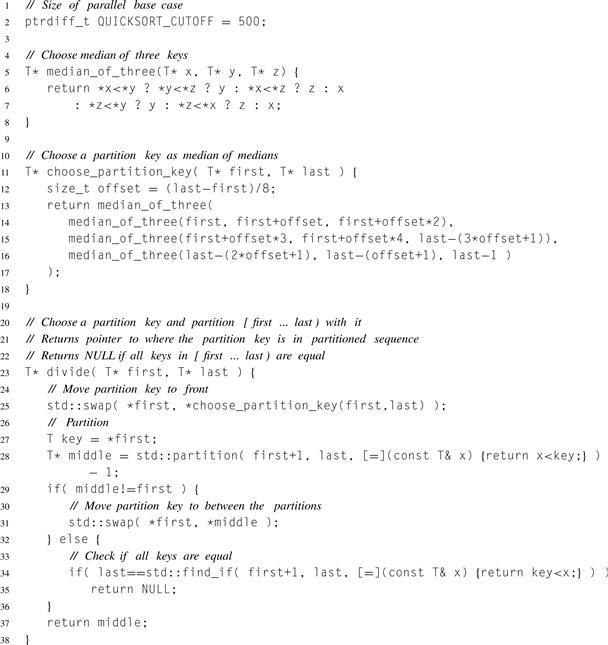
Listing 8.9 Code shared by Quicksort implementations.
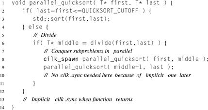
Listing 8.10 Fully recursive parallel Quicksort using Cilk Plus.
8.9.2 TBB Quicksort
TBB versions of Quicksort can be coded similarly to the Cilk Plus versions, except that the mechanics differ. A version similar to Listing 8.10 can be written using tbb::parallel_invoke to invoke pairs of recursive calls. A version similar to Listing 8.11 can be written using tbb::task_group as shown in Listing 8.12. Though in practice the code above has reasonable performance most of the time, it has a a worst-case space problem. The problem is that the Cilk Plus guarantees on space and time are not generally true in TBB, because TBB has steal-child semantics, and the guarantees depend on steal-continuation semantics (Section 8.5). In particular, if the smaller problem is consistently a single element, then ![]() tasks are added to task_group g, and none is executed until g.wait() executes. Thus, the worst case space is
tasks are added to task_group g, and none is executed until g.wait() executes. Thus, the worst case space is ![]() , even though the algorithm recurses only
, even though the algorithm recurses only ![]() deep. This is a general problem with steal-child semantics: Many children may be generated before any are run.
deep. This is a general problem with steal-child semantics: Many children may be generated before any are run.
The solution is to not generate a new child until it is needed. This can be done by simulating steal-continuation semantics in TBB, by writing the code using continuation-passing style. There are two common reasons to use continuation-passing style in TBB:
• Avoiding waiting—Instead of waiting for predecessors of a task to complete at a join point, the code specifies a continuation task to run after the join point.
• Avoiding premature generation of tasks—Instead of generating a bunch of tasks and then executing them, the code generates one task and executes it, and leaves behind a continuation that will generate the next task.
The rewritten example will have an example of each. The empty_task will represent execution after a join point. The quicksort_task will leave behind a continuation of itself.
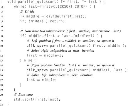
Listing 8.11 Semi-recursive parallel Quicksort using Cilk Plus. There is no cilk_sync before the base case because the base case is independent of the spawned subproblems.
Continuation-passing tasking requires using TBB’s low-level tasking interface, class tbb::task, which is designed for efficient implementation of divide-and-conquer. An instance of class task has the following information:
• A reference count of predecessor tasks that must complete before running this task. The count may include an extra one if the task is explicitly waited on. The Quicksort example does not have the wait, so the count will be exactly the number of predecessors.
• A virtual method that executes when the predecessors finish. The method may also specify the next task to execute.
• A pointer to its successor. After the method executes, the scheduler decrements the successor’s reference count. If the count becomes zero, the successor is automatically spawned.
The general steps for using it to write recursive fork–join are:
• Create a class D representing the divide/fork actions. Derive it from base class tbb::task.
• Override virtual method tbb::task::execute(). The definition should perform the divide/fork actions. It should return NULL, or return a pointer to the next task to execute.
• Create a top-level wrapper function that creates a root task and executes it using tbb::task::spawn_root_and_wait.
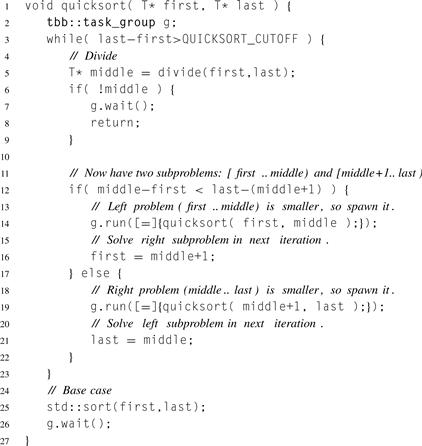
Listing 8.12 Semi-iterative parallel Quicksort using TBB.
Because of the desire to lazily generate child tasks, the Quicksort code is a little trickier than TBB code for typical fork–join situations. Listing 8.13 shows the code. Overall, the logic is similar to the Cilk Plus version in Listing 8.11, but the parallel mechanics differ. These mechanics will now be explained in detail.
The top-level routine is quicksort, which creates the root task and runs it. The root task can be viewed as the gateway from normal calling to the continuation-passing world. Instances of class task must always be allocated using an overloaded new, with an argument returned by one of the methods beginning with tbb::task::allocate. There are several of these methods, each specific to certain usages.
Class quicksort_task is a task for sorting. What were function parameters in the Cilk Plus version become class members, so that the values can be remembered between the time the task is created and when it actually runs. The override of task::execute() has the algorithm. If the task represents a base case, it does a serial sort and returns NULL. The NULL indicates that the scheduler should use its normal work-stealing algorithm for choosing the next task to execute.
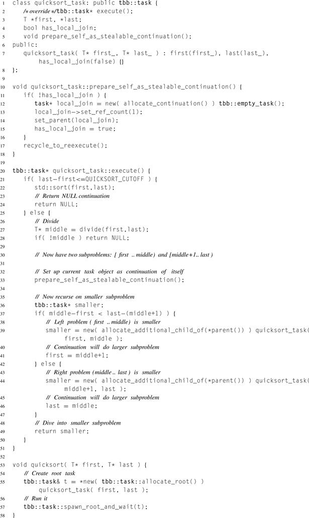
Listing 8.13 Quicksort in TBB that achieves Cilk Plus space guarantee.
If the task represents a recursive case, then it operates much like the task_group example, except that the while loop has been converted to continuation-passing style. The recursive part has been turned into the return of task smaller. The scheduler will cause the current thread to execute that task next. Sometimes this trick is used simply as an optimization to bypass the task scheduler, but here it is doing more, by forcing the current thread to dive into the smaller subproblem, just as the semi-recursive Cilk Plus version does. Meanwhile, the current task is destructively updated to become the larger subproblem. The call recycle_to_reexecute() causes it to be visible to thieves after it returns from method execute(). TBB restrictions require that this idiom be used instead of directly respawning it, because the latter could cause it to be reentrantly executed by a second thread before the first thread is done with it.
8.9.3 Work and Span for Quicksort
The average case is a bit tricky to analyze, but it turns out to be asymptotically the same as the ideal case, so the ideal case is presented here. Though ideal, it will reveal a limitation of our parallelization.
The recurrences for the ideal case, where partitioning creates subproblems of equal size, are:
![]()
The closed form solutions from the Master method are:
![]()
Thus, the speedup limit in the ideal case is:
![]()
So, the best we can expect is a logarithmic improvement in performance, no matter how many processors we throw at it.
The limit on speedup arises from the partition steps near the top levels of the recursion. In particular, the first partition step requires O (N) time. Therefore, even if the rest of the sort ran in zero time, the total time would still be O (N). To do any better, we need to parallelize the partition step, as in Sample Sort (Chapter 14), or choose a different kind of sort such as Merge Sort (Chapter 13).
However, Quicksort does have some advantages over the other sorts mentioned.
• Quicksort is an in-place algorithm. The other two sorts are not and thus have twice the cache footprint.
• Quicksort spends most of its time in std::partition, which is friendly to cache and prefetch mechanisms.
• Quicksort always moves keys via std::swap. It never copies keys. For some key types, such as reference-counted objects, swapping keys can be far faster than moving keys.
Thus, even though the other sorts have higher scalability in theory, they sometimes perform worse than Quicksort. For low core counts, parallel Quicksort may be a good choice.
8.10 Reductions and Hyperobjects
The recursive implementation of the map pattern can be extended to do reduction. Listing 8.14 shows such an extension of Listing 8.1 for doing a sum reduction of f (i) for i from lower (inclusive) to upper (exclusive).
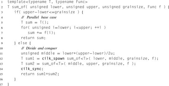
Listing 8.14 Recursive implementation of parallel reduction in Cilk Plus.
The approach extends to any operation that is associative, even if the operation is not commutative.
Using explicit fork–join for reduction is sometimes the best approach, but other times it can be a nuisance on several counts:
• The partial reduction value has to be explicit in the function prototype, either as a return value or a parameter specifying where to store it. It cannot be a global variable because that would introduce races.
• It requires writing fork–join in cases where otherwise a cilk_for would do and be easier to read.
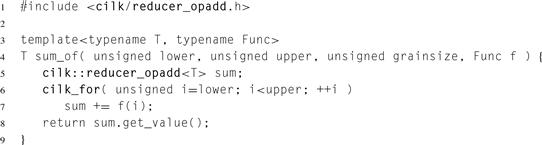
Cilk Plus hyperobjects are an elegant way to avoid these drawbacks. A hyperobject is an object for which each Cilk Plus strand gets its own view. A strand is a portion of Cilk Plus execution with no intervening fork or join points. The hyperobjects described here are called reducers because they assist doing reductions. There are other kinds of hyperobjects, such as holders and splitters, that are sometimes useful, too [FHLLB09]. Listing 8.15 shows a simple example of using a hyperobject to avoid a race.
If sum were an ordinary variable of type float, the invocations of f(1) and f(2) could race updating it and not have the correct net effect, but the code is safe because variable sum is declared as a reducer. The calls f(1) and f(2) are on different strands and so each gets its own view of sum to update.
The summation of the two views happens automatically at the cilk_sync. The Cilk Plus runtime knows to add the views because sum was declared as a reducer_opadd. Method get_value gets the value of the view. It is a method, and not an implicit conversion, so you have to be explicit about getting the value. Be sure that all strands that contribute to the value are joined before getting the value; otherwise, you may get only a partial sum.
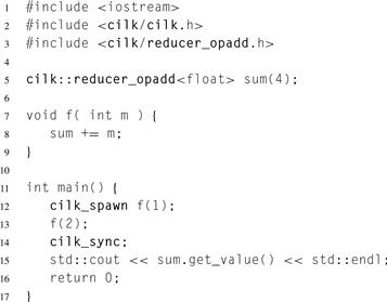
Listing 8.15 Using a hyperobject to avoid a race in Cilk Plus. Declaring sum as a reducer makes it safe to update it from separate strands of execution. The cilk sync merges the updates, so the code always prints 7.
There are other reducers built into Cilk Plus for other common reduction operations. For instance, reducer_opxor performs exclusive OR reduction. Section B.7 lists the predefined reducers. You can define your own reducer for any data type and operation that form a mathematical monoid, which is to say:
For example, the data type of strings forms a monoid under concatenation, where the identity element is the empty string. Cilk Plus provides such a reducer for C++ strings, called reducer_basic_string. Section 11.2.1 walks through the steps of building your own reducer.
Generating many views would be inefficient, so there are internal optimizations that reduce the number of views constructed. These optimizations guarantee that no more than 3P views of a hyperobject exist at any one time, where P is the total number of workers. Furthermore, new views are generated lazily, only when a steal occurs. Since steals are rare in properly written Cilk Plus code, the number of views constructed tends to be low.
Figure 8.7 illustrates this point for the example from Listing 8.15. Views are distinguished by subscripts. The left graph shows the stolen case and how only one new view has to be created. Initially variable sum has a single view sum1. If the continuation that calls f(2) is stolen, Cilk Plus creates a new view sum2 and initializes it to T(), which by convention is assumed to be the identity element. The other strand after the fork uses sum1 instead of constructing a new view. Now f(1) and f(2) can safely update their respective views. At the join point, sum2 is folded into sum1, and (not pictured) destroyed. Afterwards, sum1 has the intended total.
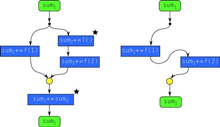
Figure 8.7 Hyperobject views in Cilk Plus. A hyperobject constructs extra view sum2 only if actual parallelism occurs. The actions marked with stars are implicit and not written by the programmer.
The right graph shows the unstolen case, in which no new views have to be created. Since the calls f(1) and f(2) run consecutively, not in parallel, a single view sum1 suffices. This is another demonstration of a general principle behind Cilk Plus: Extra effort for parallelism is expended only if the parallelism is real, not merely potential parallelism.
Listing 8.16 Using a local reducer in Cilk Plus.
Hyperobjects are handy because they are not lexically bound to parallelism constructs. They can be global variables that are updated by many different strands. The runtime will deal with reducing the updates into final correct value.
Hyperobjects are also useful as local variables, as shown in Listing 8.16, which is another way to implement the reduction from Listing 8.14.
It is important to remember that hyperobjects eliminate races between strands of Cilk Plus execution, not races between arbitrary threads. If multiple threads not created by the Cilk Plus runtime do concurrently access a hyperobject, they will race and thus possibly introduce non-determinism.
8.11 Implementing Scan with Fork–Join
This section shows how to use fork–join to implement the scan pattern using the interface presented in Section 5.4. The code examples are Cilk Plus. The TBB template parallel_scan uses a similar implementation technique but with a twist described later.
The parallel scan algorithm [Ble93] operates as if the data are the leaves of a tree as shown in Figure 8.8. In the picture, the input consists of the sequence ![]() and an initial value initial, and the output sequence is an exclusive scan
and an initial value initial, and the output sequence is an exclusive scan ![]() . The algorithm makes two sweeps over the tree, one upward and one downward. The upsweep computes a set of partial reductions of the input over tiles. The downsweep computes the final scan by combining the partial reduction information. Though the number of tiles in our tree illustration is a power of two, the example code works for any number of tiles.
. The algorithm makes two sweeps over the tree, one upward and one downward. The upsweep computes a set of partial reductions of the input over tiles. The downsweep computes the final scan by combining the partial reduction information. Though the number of tiles in our tree illustration is a power of two, the example code works for any number of tiles.
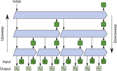
Figure 8.8 Tree for parallel scan. Parallel scan does two passes over the tree, one upward and one downward. See Figure 8.9 for the internal structure of the pentagonal tree nodes.
Figure 8.9 shows the internal structure of a tree node. Let ⊕ denote the combiner operation. The term subscan here means a subsequence of the final scan sequence. The node shown computes values related to the subscan for ![]() . The subsequence is split into two halves: a leading subsequence of k elements and a trailing subsequence of
. The subsequence is split into two halves: a leading subsequence of k elements and a trailing subsequence of ![]() elements. Let
elements. Let ![]() denote a reduction over m consecutive elements of the sequence, starting at index i. During the upsweep, the node computes
denote a reduction over m consecutive elements of the sequence, starting at index i. During the upsweep, the node computes ![]() . Let
. Let ![]() denote the initial value required for computing the subscan starting at index i. In other words,
denote the initial value required for computing the subscan starting at index i. In other words, ![]() . During the downsweep, the node gets
. During the downsweep, the node gets ![]() from its parent, passes it downward, and computes
from its parent, passes it downward, and computes ![]() . These are the initial values for computing the subscans for the two half subsequences.
. These are the initial values for computing the subscans for the two half subsequences.
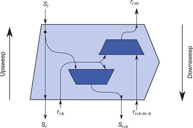
Figure 8.9 Node in the parallel scan tree in Figure 8.8. Each operation costs one invocation of the combining functor. For an n-ary tree, the node generalizes to performing an n-element reduction during the upsweep and a n-element exclusive scan on the downsweep.
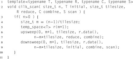
Listing 8.17 Top-level code for tiled parallel scan. This code is actually independent of the parallel framework. It allocates temporary space for partial reductions and does an upsweep followed by a downsweep.
The tree computes an untiled exclusive scan. A tiled exclusive scan for an operation ⊕ can be built from it as follows. Label the tiles b1, b2, …, bN−1. Conceptually, the steps are:
1. Compute each rk as the ![]() reduction of tile bk.
reduction of tile bk.
2. Do upsweep and downsweep to compute each sk.
3. Compute the exclusive scan of tile bk using sk as the initial value.
In practice, Steps steps 1 and and 3 are not separate passes, but embedded into the upsweep and downsweep passes, respectively. For an inclusive scan, change the last step to be an inclusive scan over each tile.
Listing 8.17 shows the top-level code for a tiled scan. The parameters are explained in Section 5.4 on page 164. As noted in that section, the reduction is done for the last tile even though its return value is unnecessary in order to permit fusion optimization.
Listing 8.18 shows the code for routine upsweep. It performs the upsweep for the index range i:m. The base case invokes the tile reduction functor reduce. The recursive case chooses where to split the index space, using function split (not shown), which should return the greatest power of two less than m:
![]()
The function serves to embed an implicit binary tree onto the index space. The if at the end of routine upsweep checks whether there is a tree node summarizing the index space. When m is not a power of two, there is no such node. Conceptually the missing node is for summarizing an index space larger than the requested space.
Listing 8.19 shows the code for routine downsweep. Most of the parameters are similar to those in the other routines. Parameter lastsize is the size of the rightmost tile, which might be a partial tile. Its structure closely resembles the structure of upsweep because it is walking the same tree, only it does its real work before the fork, not after the join as in upsweep. Consequently, tail recursion optimization (Section 8.3) can be applied to downsweep but not upsweep.
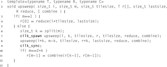
Listing 8.18 Upsweep phase for tiled parallel scan in Cilk Plus.
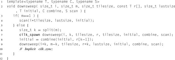
Listing 8.19 Downsweep phase for tiled parallel scan in Cilk Plus.
The work is proportional to the number of nodes in the tree, and the span is proportional to the height of the tree. So the asymptotic work-span bounds are
![]()
Unfortunately the asymptotic bounds hide a constant factor of 2 in the work, and in practice this factor of 2 can undo much of the gains from parallelization. A serial scan makes a single pass over the data, but a parallel scan makes two passes: upsweep and downsweep. Each pass requires reading the data. Hence, for large scans where data does not fit in cache, the communication cost is double that for a serial scan. Therefore, when communication bandwidth is the limiting resource for a serial scan, a parallel scan will run half as fast. Even if it does fit in the total aggregate cache, there is a communication problem, because greedy scheduling arbitrarily assigns workers to the tile reductions and scan reductions. Thus, each tile is often transferred from the cache of the worker who reduced it to the cache of the worker who scans it.
The implementation of TBB’s tbb::parallel_scan attempts to mitigate this issue through a trick that dynamically detects whether actual parallelism is available. The TBB interface requires that each tile scan return a reduction value as well. This value is practically free since it is computed during a scan anyway. During the upsweep pass, the TBB implementation uses the tile scan instead of a reduction whenever it has already computed all reductions to the left of the tile. This enables skipping the downsweep pass for all tiles to the left of all tiles processed by work-stealing thieves. In other words, execution is equivalent to a tiled serial scan until the point is reached where actual parallelism forks the control flow. This way, if two workers are available, typically only the right half of the tree needs two passes, thus averaging 1.5 passes over the data. For more available workers, the benefit starts to diminish. The trick is dynamic—tbb::parallel_scan pays the 2× overhead for parallelism only if actual parallelism is being applied to the scan.
One elegant feature of our Cilk Plus interface for scan is that sometimes the scan values can be consumed without actually storing them. For example, consider implementing the pack pattern using a scan followed by a conditional scatter, as described in Section 6.4. Listing 8.20 shows the code.
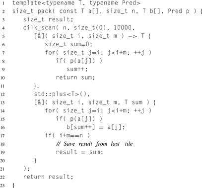
Listing 8.20 Implementing pack pattern with cilk_scan from Listing 8.17.
It fills an array b with the elements of array a that satisfy predicate p and returns the number of such elements found. It calls parallel_scan to compute a running sum of how many elements satisfy predicate p. A standalone scan of the sum operation would have to store the partial sums in an array. That is not necessary here, because each partial sum is consumed immediately by the assignment b[sum++] − a[j].
The scan tree in Figure 8.8 generalizes to trees of higher degree. For an N-ary scan tree, the node performs an N-ary serial reduction during the upsweep and an N-element serial exclusive scan on the downsweep. Indeed, some implementations do away with recursion altogether and use a single serial scan, as was shown by the OpenMP implementation of scan in Section 5.4. That saves synchronization overhead at the expense of increasing the span. If such a degenerate single-node tree is used for a tiled scan with tiles of size ![]() , the span is
, the span is ![]() . Though not as good as the
. Though not as good as the ![]() span using a binary tree, it is an improvement over the
span using a binary tree, it is an improvement over the ![]() time for a serial scan, and constant factors can put it ahead in some circumstances.
time for a serial scan, and constant factors can put it ahead in some circumstances.
8.12 Applying Fork–Join to Recurrences
Recurrences, described in Section 7.5, result when a loop nest has loop-carried dependencies—that is, data dependencies on outputs generated by earlier iterations in the serial execution of a loop. We explained how this can always be parallelized with a hyperplane sweep. However, sometimes a recurrence can also be evaluated using fork–join by recursively partitioning the recurrence, an approach that can have useful data locality properties. This section explores some tradeoffs for recursive partitioning.
For example, consider the “binomial lattice” recurrence in Figure 8.10. For the sake of a familiar example, the values shown are binomial coefficients, organized as in Pascal’s triangle. However, this particular pattern of dependencies shows up in far more sophisticated applications such as pricing models for stock options, infinite impulse response image processing filters, and in dynamic programming problems. A good example of the last is the Smith–Waterman algorithm for sequence alignment, which is used extensively in bioinformatics [SW81].
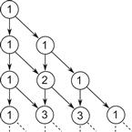
Figure 8.10 Directed acyclic data dependency graph for binomial lattice.
This data dependency graph is an obvious candidate for the superscalar or “fire when ready” approach, but using this approach would give up the locality and space advantages of fork–join. A recursive fork–join decomposition of this recurrence will be explored as an alternative, and its advantages and disadvantages analyzed.
Consider a diamond-shaped subgraph where the number of points along an edge is a power of two, such as the example in Figure 8.11. The diamond can be decomposed into four subdiamonds, labeled D0, D1, D2, and D3. Diamonds D2 and D3 can be evaluated in parallel. Furthermore, the same approach can be applied recursively to the four subdiamonds.
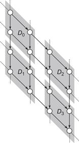
Figure 8.11 Decomposing a diamond subgraph into subdiamonds.
The parallel base case occurs when the current diamond is so small that fork–join overheads become significant. At that point, vector parallelism can be exploited by serially iterating over the diamond from top to bottom and computing each row of points in parallel.
Here is a pseudocode sketch for the recursive pattern:
void recursive_diamond( diamond D) {
if(D is small ) {
base_diamond(D);
} else {
divide D into subdiamonds D0, D1, D2, D3;
recursive_diamond(D0);
cilk_spawn recursive_diamond(D1);
/* nospawn */recursive_diamond(D2);
cilk_sync;
recursive_diamond(D3)
}
}
The effort for turning this sketch into efficient code mostly concerns manipulation of memory. There is a fundamental tradeoff between parallelism and worst-case memory space, because in order to avoid a race operations occurring in parallel must record their results into separate memory locations. For the binomial lattice, one extreme is to use a separate memory location for each lattice point. This is inefficient. For a diamond with a side of width w, it requires ![]() space.
space.
At the other extreme, it is possible to minimize space by mapping an entire column of lattice points to a single memory location. Unfortunately this mapping requires serial execution, to avoid overwriting a location with a new value before all uses of its old value complete, as shown below:
void base_diamond( diamond D) {
for each row R in D do
for each column i in row R from right to left
A[i]=f(A[i-1],A[i]);
}
This serialization extends to the recursive formulation: Diamond D1 must be evaluated before D2, and hence fork–join parallelism could not be used.
The solution is to double the space and have two locations for each lattice point. Organize the locations into two arrays, A and B. A location in array A corresponds to a column of the lattice. A location in array B corresponds to a diagonal of the lattice. Subscripts for B start at zero and go downward for the sake of improving vectorization of the base case, as explained later.
Figure 8.12 shows the parameterized description of a diamond subgraph:
• a points to the element of A holding the leftmost column value.
• b points to the element of B holding the topmost diagonal value.
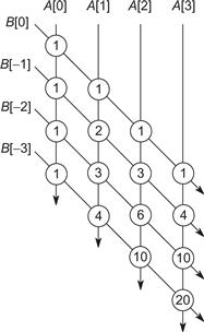
Figure 8.12 Parameters for diamond subgraph.
• w is the number of points along a side of the diamond.
• s and n describe clipping limits on the diamond. The rows to be processed, relative to the top corner, are rows with indices in the half-open interval [s,n).
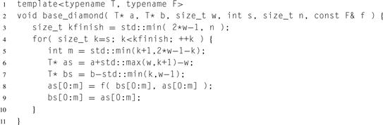
Listing 8.21 Base case for evaluating a diamond of lattice points.
Listing 8.21 shows the code for the row updates, using vector parallelism across each row. The two vector updates can in theory be chained together. However, at the time of writing, Cilk Plus did not allow chaining of such assignments, though they will be allowed in the future.
With a positive coordinate convention for B, the vector update would look something like:
as[0:m] = f(bs[0:m:-1], as[0:m]);
bs[0:m:-1] = as[0:m];
with pointer bs being calculated slightly differently. Though the code would work, it would be less efficient because the compiler would have to insert permutation instructions to account for the fact that as and bs have strides in different directions.
Listing 8.22 shows the rest of the code. It assumes that only the topmost diamond is clipped.
One final note: Additional performance can be gained by turning off denormalized floating point (“denormals”) numbers. Their use can severely impact performance. Floating point numbers consist of a mantissa and exponent; the normalized format has a mantissa that always has a leading one (value = 1.mantissaexponent), whereas a denormalized format has a leading zero (value = 0.mantisssaexponent). Denormalized floating point numbers are so small (close to zero) that the exponent would underflow in the normal representation without this additional “denormal” format. Denormalized numbers help preserve important algebraic properties such as the equivalence of the equality tests x − y = 0 and x = y. Alas, denormalized numbers often require extra cycles to process. A common case of f in our example is a function that averages its inputs, which will result in the output being a bell curve. The tails of the curve will have values that asymptotically approach zero and consequently contain many denormalized floating-point values. Using options that flush denormalized numbers to zero, such as /Qftz with the Intel compiler, can greatly improve the performance of this example. This is very useful if the value of the extra numerical range is not worth the performance loss to your program. It is common to use such flush-to-zero options in high-performance code.
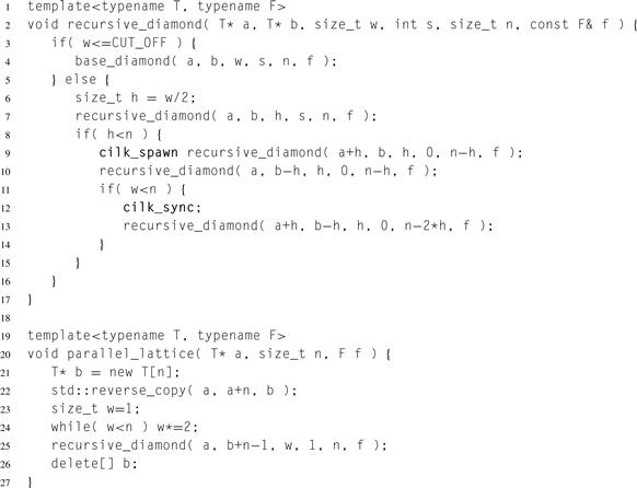
Listing 8.22 Code for parallel recursive evaluation of binomial lattice in Cilk Plus.
8.12.1 Analysis
The work T1 for the diamond lattice is ![]() . The corresponding span
. The corresponding span ![]() for the same algorithm is
for the same algorithm is ![]() . Taking the ratio of these two results in a speedup of
. Taking the ratio of these two results in a speedup of ![]() . By inspection, it is easy to see that if the recurrence was executed directly by following graph edges, then the span is only
. By inspection, it is easy to see that if the recurrence was executed directly by following graph edges, then the span is only ![]() and speedup is
and speedup is ![]() . The point is that imposing the recursive diamond structure has improved data locality but lengthened the asymptotic span. The practical impact will depend on the number P of available processors. If P is significantly less than N0.415, the impact will be relatively small; otherwise, it may be large compared to the direct solution. However, constant factors due to the better arithmetic intensity (and therefore better cache behavior) of the tiled version may allow it to perform better in practice. Unfortunately, which is better will depend on the magnitude of the relevant constant factors on a particular architecture, so the best solution often involves selecting an implementation and tuning its parameters by experimentation.
. The point is that imposing the recursive diamond structure has improved data locality but lengthened the asymptotic span. The practical impact will depend on the number P of available processors. If P is significantly less than N0.415, the impact will be relatively small; otherwise, it may be large compared to the direct solution. However, constant factors due to the better arithmetic intensity (and therefore better cache behavior) of the tiled version may allow it to perform better in practice. Unfortunately, which is better will depend on the magnitude of the relevant constant factors on a particular architecture, so the best solution often involves selecting an implementation and tuning its parameters by experimentation.
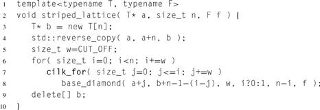
Listing 8.23 Marching over diamonds in Cilk Plus. This is an example of a hyperplane sweep parallelization of the binomial lattice recurrence.
8.12.2 Flat Fork–Join
Another solution to consider is to march over the lattice from top to bottom and execute a row of diamonds in parallel using a hyperplane sweep. This is row-by-row application of the map pattern, and is discussed in Section 7.5. Listing 8.23 shows the code for this approach, which uses routine base_diamond from Listing 8.21.
A cilk_for with K iterations takes time ![]() . Thus,
. Thus, ![]() , which for large N is a significant improvement over
, which for large N is a significant improvement over ![]() and only a factor of
and only a factor of ![]() away from the optimal span of
away from the optimal span of ![]() .
.
8.13 Summary
In this chapter we presented the fork–join pattern, which is a natural fit for parallel divide-and-conquer algorithms. Parallel divide-and-conquer generates independent subproblems, solves them in parallel, and then combines the results. Algorithms based on recursive divide-and-conquer often have very good space behavior, locality, and load-balancing properties when executed by a fork–join implementation that uses work-stealing. Speedup may, however, be limited by the speed of the divide or combine steps or by uneven division of work.
We presented the Master method for computing the asymptotic complexity of the work and span. These can be used to predict the speedup of a divide-and-conquer algorithm. Karatsuba polynomial multiplication and Quicksort were given as examples, which also demonstrated practical issues with memory allocation.
Cache-oblivious algorithms using matrix multiplication as an example were discussed, and we also presented fork–join implementations of scan and the binomial lattice recurrence.
1 TBB cannot make the same guarantee unless the code is written in continuation-passing style, an example of which is given in Section 8.9.2.
2 Splits could be quantized to the cache line granularity, though then the code would no longer be completely cache oblivous.