
Chapter 3
Patterns
Patterns have become popular recently as a way of codifying best practices for software engineering [GHJV95]. While patterns were originally applied to object-oriented software, the basic idea of patterns—identifying themes and idioms that can be codified and reused to solve specific problems in software engineering—also applies to parallel programming. In this book, we use the term parallel pattern to mean a recurring combination of task distribution and data access that solves a specific problem in parallel algorithm design.
A number of parallel patterns are described in this book. We will characterize and discuss various algorithms in terms of them. We give each pattern a specific name, which makes it much easier to succinctly describe, discuss, and compare various parallel algorithms. Algorithms are typically designed by composing patterns, so a study of patterns provides a high-level “vocabulary” for designing your own algorithms and for understanding other people’s algorithms.
This chapter introduces all of the patterns discussed in this book in one place. We also introduce a set of serial patterns for comparison because parallel patterns are often composed with, or generalized from, these serial patterns. The serial patterns we discuss are the foundation of what is now known as structured programming. This helps make clear that the pattern-based approach to parallel programming used in this book can, to some extent, be considered an extension of the idea of structured programming.
It should be emphasized that patterns are universal. They apply to and can be used in any parallel programming system. They are not tied to any particular hardware architecture, programming language, or system. Patterns are, however, frequently embodied as mechanisms or features of particular systems. Systems, both hardware and software, can be characterized by the parallel patterns they support. Even if a particular programming system does not directly support a particular pattern it can usually, but not always, be implemented using other features.
In this book, we focus on patterns that lead to well-structured, maintainable, and efficient programs. Many of these patterns are in fact also deterministic, which means they give the same result every time they are executed. Determinism is a useful property since it leads to programs that are easier to understand, debug, test, and maintain.
We do not claim that we have covered all possible parallel patterns in this book. However, the patterns approach provides a framework into which you can fit additional patterns. We intend to document additional patterns online as a complement to this book, and you might also discover some new patterns on your own. In our experience many “new” patterns are in fact variations, combinations, or extensions of the ones we introduce here. We have focused in this book on the most useful and basic patterns in order to establish a solid foundation for further development.
We also focus on “algorithm strategy” patterns, sometimes called algorithmic skeletons [Col89, AD07]. These patterns are specifically relevant to the design of algorithm kernels and often appear as programming constructs in languages and other systems for expressing parallelism. Patterns have also been referred to as motifs and idioms. In more comprehensive pattern languages [MSM04, ABC+06], additional patterns and categories of patterns at both higher and lower levels of abstraction are introduced. The OUR pattern language in particular is quite extensive [Par11].
We have focused on the class of algorithm strategy patterns because these are useful in the design of machine-independent parallel algorithms. Algorithm strategy patterns actually have two parts, a semantics, which is what they accomplish, and an implementation, which is how they accomplish it. When designing an algorithm, you will often want to think only about the semantics of the pattern. However, when implementing the algorithm, you have to be aware of how to implement the pattern efficiently. The semantics are machine-independent but on different kinds of hardware there may be different implementation approaches needed for some of the patterns. We will discuss some of these low-level implementation issues in later chapters; in this chapter, we focus mostly on the semantics.
This chapter may seem a little abstract. In order to keep this chapter compact we do not give many examples of the use of each pattern here, since later chapters will provide many specific examples. If you would like to see more concrete examples first, we recommend that you skip or skim this chapter on first reading and come back to read it later.
3.1 Nesting Pattern
The nesting pattern is the fundamental compositional pattern and appears in both serial and parallel programs. Nesting refers to the ability to hierarchically compose patterns.
The nesting pattern simply means that all “task blocks” in our pattern diagrams are actually locations within which general code can be inserted. This code can in turn be composed of other patterns. This concept is demonstrated in Figure 3.1.
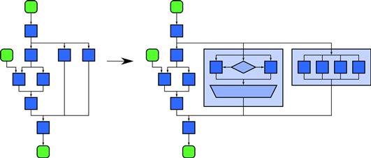
Figure 3.1 Nesting pattern. This is a compositional pattern that allows other patterns to be composed in a hierarchy. The definition of nesting is that any task block in a pattern can be replaced with a pattern with the same input and output configuration and dependencies.
Nesting allows other parallel patterns to be composed hierarchically, and possibly recursively. Ideally, patterns can be nested to any depth and the containing pattern should not limit what other patterns can be used inside it. Not all patterns support nesting. In this book, we focus on patterns that do support nesting since it is important for creating structured, modular code. In particular, it is hard to break code into libraries and then compose those libraries into larger programs unless nesting is supported. Programming models that do not support nesting likewise will have difficulties supporting modularity.
Figure 3.1 also demonstrates the graphical conventions we use to explain patterns generally. As previously described in Figure 2.1, tasks, which describe computations, are shown as sharp-cornered boxes, while data are indicated by round-cornered boxes. Grouped data is indicated by round-cornered enclosures, and grouped tasks are indicated by sharp-cornered polygonal enclosures. For some patterns we will introduce additional symbols in the form of various polygonal shapes.
Ordering dependencies are given by arrows. Time goes from top to bottom, and except when representing iteration we avoid having arrows go upward and therefore “backward” in time. In the absence of such upward arrows, the height of a pattern diagram is a rough indication of the span (see Section 2.5.7) of a pattern. These graphical conventions are intentionally similar to those commonly associated with flow-charts.
The nesting pattern basically states that the interior of any “task box” in this notation can be replaced by any other pattern. Nesting can be static (related to the code structure) or dynamic (recursion, related to the dynamic function call stack). To support dynamic data parallelism, the latter is preferred, since we want the amount of parallelism to grow with problem size in order to achieve scalability. If static nesting is used, then nesting is equivalent to functional decomposition. In that case, nesting is an organizational structure for modularity but scaling will be achieved by the nested patterns, not by nesting itself.
Structured serial programming is based on nesting the sequence, selection, iteration, and recursion patterns. Likewise, we define structured parallel programming to be based on the composition of nestable parallel patterns. In structured serial programming, goto is avoided, since it violates the orderly arrangement of dependencies given by the nesting pattern. In particular, we want simple entry and exit points for each subtask and want to avoid jumping out of or into the middle of a task. Likewise, for “structured parallel programming” you should use only patterns that fit within the nesting pattern and avoid additional dependencies, both data and control, that break this model.
Nesting, especially when combined with recursion, can lead to large amounts of potential parallelism, also known as parallel slack. This can either be a good thing or a bad thing. For scalability, we normally want a large amount of parallel slack, as discussed in Section 2.5.
However, hardware resources are finite. It is not a good idea to blindly create threads for all of the potential parallelism in an application, since this will tend to oversubscribe the system. The implementation of a programming system that efficiently supports arbitrary nesting must intelligently map potential parallelism to actual physical parallelism. Since this is difficult, several programming models at present support only a fixed number of nesting levels and may even map these levels directly onto hardware components.
This is unfortunate since composability enables the use of libraries of routines that can be reused in different contexts. With a fixed hierarchy, you have to be aware at what level of the hierarchy any code you write will be used. Mapping the hierarchy of the program directly onto the hardware hierarchy also makes code less future-proofed. When new hardware comes out, it may be necessary to refactor the hierarchy of patterns to fit the new hardware.
Still, many systems are designed this way, including OpenCL, CUDA, C++ AMP, and to some extent OpenMP. Some of these programming systems even encode the physical hierarchy directly into keywords in the language, making future extension to more flexible hierarchies difficult.
In contrast, both Cilk Plus and TBB, discussed in this book, can support arbitrary nesting. At the same time, these systems can do a good job of mapping potential parallelism to actual physical parallelism.
3.2 Structured Serial Control Flow Patterns
Structured serial programming is based on four control flow patterns: sequence, selection, iteration, and recursion. Several parallel patterns are generalizations of these. In addition, these can be nested hierarchically so the compositional “nesting” pattern is also used.
We discuss these in some detail, even though they are familiar, to point out the assumptions that they make. It is important to understand these assumptions because when we attempt to parallelize serial programs based on these patterns, we may have to violate these assumptions.
3.2.1 Sequence
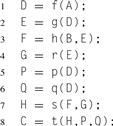
A sequence is a ordered list of tasks that are executed in a specific order. Each task is completed before the one after it starts. Suppose you are given the serial code shown in Listing 3.1. This code corresponds to Figure 3.2. Function f in line 1 will execute before function g in line 2, which will execute before function h in line 3. A basic assumption of the sequence pattern is that the program text ordering will be followed, even if there are no data dependencies between the tasks, so that side effects of the tasks such as output will also be ordered. For example, if task f outputs “He”, task g outputs “llo” and task h outputs “World”, then the above sequence will output “Hello World” even if there were no explicit dependencies between the tasks.
![]()
Listing 3.1 Serial sequence in pseudocode.
![]()
Figure 3.2 Sequence pattern. A serial sequence orders operations in the sequence in which they appear in the program text.
In Listing 3.2, data dependencies happen to restrict the order to be the same as the texture order. However, if the code happened to be as shown in Listing 3.2, the sequence pattern would still require executing g after f, as shown in Figure 3.3, even though there is no apparent reason to do so. This is so side effects, such as output, will still be properly ordered.
![]()
Listing 3.2 Serial sequence, second example, in pseudocode.

Listing 3.3 Serial selection in pseudocode.
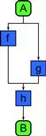
Figure 3.3 Sequence pattern, second example. A serial sequence orders operations in the sequence in which they appear in the program text, even if there are no apparent dependencies between tasks. Here, since g comes after f in the program text, the sequence pattern requires that they be executed in that order, even though there is no explicit dependency.
There is a parallel generalization of sequence, the superscalar sequence discussed in Section 3.6.1, which removes the “code text order” constraint of the sequence pattern and orders tasks only by data dependencies. In fact, as discussed in Section 2.4, modern out-of-order processors do often reorder operations and do not strictly follow the sequence pattern.
3.2.2 Selection
In the selection pattern, a condition c is first evaluated. If the condition is true, then some task a is executed. If the condition is false, then task b is executed. There is a control-flow dependency between the condition and the tasks so neither task a nor b is executed before the condition has been evaluated. Also, exactly one of a or b will be executed, never both; this is another fundamental assumption of the serial selection pattern. See Figure 3.4. In code, selection will often be expressed as shown in Listing 3.3.
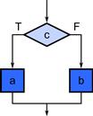
Figure 3.4 Selection pattern. One and only one of two alternatives a or b is executed based on a Boolean condition c.
There is a parallel generalization of selection, the speculative selection pattern, which is discussed in Section 3.6.3. In speculative selection all of a, b, and c may be executed in parallel, but the results of one of a or b are discarded based on the result of computing c.
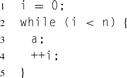
3.2.3 Iteration
In the iteration pattern, a condition c is evaluated. If it is true, a task a is evaluated, then the condition c is evaluated again, and the process repeats until the condition becomes false. This is diagrammed in Figure 3.5.
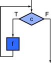
Figure 3.5 Serial iteration pattern. The task f is executed repeatedly as long as the condition c is true. When the condition becomes false, the tasks following this pattern are executed.
Unlike our other pattern diagrams, for iteration we use arrows that go “backward” in time. Since the number of iterations is data dependent, you cannot necessarily predict how many iterations will take place, or if the loop will even terminate. You cannot evaluate the span complexity of an algorithm just by looking at the height of the diagram. Instead, you have to (conceptually) execute the program and look at the height of the trace of the execution.
![]()
Listing 3.4 Iteration using a while loop in pseudocode.
![]()
Listing 3.5 Iteration using a for loop in pseudocode.
This particular form of loop (with the test at the top) is often known as a while loop. The while loop can of course be expressed in code as shown in Listing 3.4.
There are various other forms of iteration but this is the most general. Other forms of looping can be implemented in terms of the while loop and possibly other patterns such as sequence.
The loop body a and the condition c normally have data dependencies between them; otherwise, the loop would never terminate. In particular, the loop body should modify some state that c uses for termination testing.
One complication with parallelizing the iteration pattern is that the body task f may also depend on previous invocations of itself. These are called loop-carried dependencies. Depending on the form of the dependency, loops may be parallelized in various ways.
One common form of loop is the counted loop, sometimes referred to simply as a for loop, which also generates a loop index, as shown in Listing 3.5.
Listing 3.6 Demonstration of while/for equivalence in pseudocode.
This is equivalent to the while loop shown in Listing 3.6. Note that the loop body now has a loop-carried dependency on i. Even so, there are various ways to parallelize this specific form of loop, based on the fact that we know all the loop indices for every iteration in advance and can compute them in parallel. This particular loop form also has a termination condition based on a count n known in advance, so we can actually compute its complexity as a function of n.
Many systems for parallelizing loops, including Cilk Plus and OpenMP, prohibit modifications to i or n in the body of loops in the form of Listing 3.5; otherwise, the total number of iterations would not be known in advance. Serial loops do not have this prohibition and allow more general forms of termination condition and index iteration.
Several parallel patterns can be considered parallelizations of specific forms of loops include map, reduction, scan, recurrence, scatter, gather, and pack. These correspond to different forms of loop dependencies. You should be aware that there are some forms of loop dependencies that cannot be parallelized. One of the biggest challenges of parallelizing algorithms is that a single serial construct, iteration, actually maps onto many different kinds of parallelization strategies. Also, since data dependencies are not as important in serial programming as in parallel programming, they can be hidden.
In particular, the combination of iteration with random memory access and pointers can create complex hidden data dependencies. Consider the innocent-looking code in Listing 3.7. Can this code be parallelized or not?
The answer is … maybe. In fact, the data dependencies are encoded in the arrays a, b, c, and d, so the parallelization strategy will depend on what values are stored in these arrays.1 This code is, in fact, an interpreter for a simple “programming language” and can do relatively arbitrary computation. You have to decode the data dependency graph of the “program” stored in arrays a, b, c, and d before you know if the code can be parallelized! Such “accidental interpreters” are surprisingly common.
Other complications can arise due to pointers. For example, suppose we used the slightly different version of the code in Listing 3.8. The difference is that we output to a new argument y, in an attempt to avoid the data dependencies of the previous example. Can this version of the code be parallelized?
The answer is … maybe. The array inputs x and y are really pointers in C. The code can be parallelized if x does not point to the same location as y (or overlapping locations). If they do, we say the inputs are aliased, and this example has effectively the same data dependencies as Listing 3.7. So, now the parallelization of this function depends on how we call it. However, even if x and y point to distinct regions of memory, we still may not be able to parallelize safely if there are duplicate values in a, since race conditions can result from parallel writes to the same memory location. We will discuss the problem of parallel random writes in Section 3.5.5.
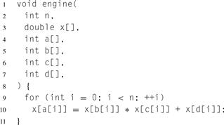
Listing 3.7 A difficult example in C. Can this code be parallelized?
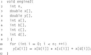
Listing 3.8 Another difficult example in C. Can this code be parallelized?
3.2.4 Recursion
Recursion is a dynamic form of nesting which allows functions to call themselves, directly or indirectly. It is usually associated with stack-based memory allocation or, if higher-order functions are supported, closures (see Section 3.4.4) which are objects allocated on the heap. Tail recursion is a special form of recursion that can be converted into iteration, a fact that is important in functional languages which often do not support iteration directly. In tail recursion, the calling function returns immediately after the recursive call and returns the value, if any, returned by the recursive call without modification.
3.3 Parallel Control Patterns
Parallel control patterns extend the serial control patterns presented in Section 3.2. Each parallel control pattern is related to one or more of the serial patterns but relaxes the assumptions of the serial control patterns in various ways, or is intended for parallelizing a particular configuration of some serial control pattern.
3.3.1 Fork–Join
The fork–join pattern lets control flow fork into multiple parallel flows that rejoin later. Various parallel frameworks abstract fork–join in different ways. Some treat fork–join as a parallel form of a compound statement; instead of executing substatements one after the other, they are executed in parallel. Some like OpenMP’s parallel region fork control into multiple threads that all execute the same statement and use other constructs to determine which thread does what.
Another approach, used in Cilk Plus, generalizes serial call trees to parallel call trees, by letting code spawn a function instead of calling it. A spawned call is like a normal call, except the caller can keep going without waiting for the callee to return, hence forking control flow between caller and callee. The caller later executes a join operation (called “sync” in Cilk Plus) to wait for the callee to return, thus merging the control flow. This approach can be implemented with an efficient mechanism that extends the stack-oriented call/return mechanism used for serial function calls.
Fork–join should not be confused with barriers. A barrier is a synchronization construct across multiple threads. In a barrier, each thread must wait for all other threads to reach the barrier before any of them leave. The difference is that after a barrier all threads continue, but after a join only one does. Sometimes barriers are used to imitate joins, by making all threads execute identical code after the barrier, until the next conceptual fork.
The fork–join pattern in Cilk Plus is structured in that the task graph generated is cleanly nested and planar, so the program can be reasoned about in a hierarchical fashion. When we refer to the fork–join pattern in this book we will be specifically referring to this structured form.
3.3.2 Map
As shown in Figure 3.6, the map pattern replicates a function over every element of an index set. The index set may be abstract or associated with the elements of a collection. The function being replicated is called an elemental function since it applies to the elements of an actual collection of input data. The map pattern replaces one specific usage of iteration in serial programs: a loop in which every iteration is independent, in which the number of iterations is known is advance, and in which every computation depends only on the iteration count and data read using the iteration count as an index into a collection. This form of loop is often used, like map, for processing every element of a collection with an independent operation. The elemental function must be pure (that is, without side-effects) in order for the map to be implementable in parallel while achieving deterministic results. In particular, elemental functions must not modify global data that other instances of that function depend on.
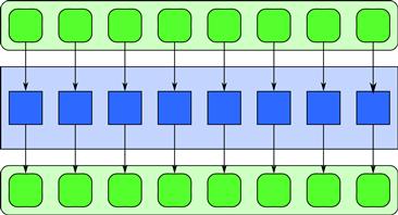
Figure 3.6 Map pattern. In a map pattern, a function is applied to all elements of a collection, usually producing a new collection with the same shape as the input.
Examples of use of the map pattern include gamma correction and thresholding in images, color space conversions, Monte Carlo sampling, and ray tracing.
3.3.3 Stencil
The stencil pattern is a generalization of the map pattern in which an elemental function can access not only a single element in an input collection but also a set of “neighbors.” As shown in Figure 3.7, neighborhoods are given by set of relative offsets.
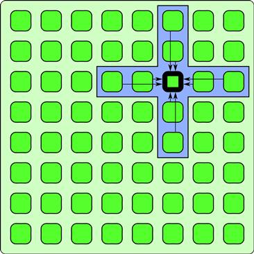
Figure 3.7 Stencil pattern. A collection of outputs is generated, each of which is a function of a set of neighbors in an input collection. The locations of the neighbors are located in a set of fixed offsets from each output. Here, only one neighborhood is shown, but in actuality the computation is done for all outputs in parallel, and different stencils can use different neighborhoods. Elements along the boundaries require special handling.
Optimized implementation of the stencil uses tiling to allow data reuse, as is discussed in detail in Section 7.3.
The stencil pattern is often combined with iteration. In this case, a stencil is repeated over and over to evolve a system through time or to implement an iterative solver. The combined pattern is equivalent to a space–time recurrence and can be analyzed and optimized using the techniques for the recurrence pattern, as discussed in Sections 3.3.6 and 7.5.
For the stencil pattern, boundary conditions on array accesses need to be considered. The edges of the input need require special handling either by modifying the indexing for out-of-bounds accesses or by executing special-case versions of the elemental function. However, the implementation should avoid using this special-case code in the interior of the index domain where no out-of-bounds accesses are possible.
The stencil pattern is used for image filtering, including convolution, median filtering, motion estimation in video encoding, and isotropic diffusion noise reduction. The stencil pattern is also used in simulation, including fluid flow, electromagnetic and financial partial differential equation (PDE) solvers, lattice quantum chromodynamics (QCD), and cellular automata (including lattice Boltzmann flow flow solvers). Many linear algebra operations can also be seen as stencils.
3.3.4 Reduction
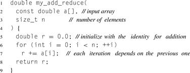
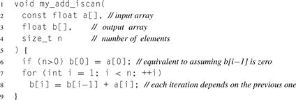
A reduction combines every element in a collection into a single element using an associative combiner function. Given the associativity of the combiner function, many different orderings are possible, but with different spans. If the combiner function is also commutative, additional orderings are possible. A serial implementation of reduction, using addition as the combiner function and a sequential ordering, is given in Listing 3.9. The ordering of operations used in this code corresponds to Figure 3.8. Such a reduction can be used to find the sum of the elements of a collection, a very common operation in numerical applications.
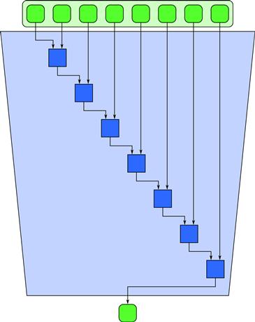
Figure 3.8 Serial reduction pattern. A reduction combines all the elements in a collection into a single element using an associative combiner function. Because the combiner function is associative, many orderings are possible. The serial ordering shown here corresponds to Listing 3.9. It has span n, so no parallel speedup is possible.
Although Listing 3.9 uses a loop with a data dependency, Figure 3.9 shows how a reduction can be parallelized using a tree structure. The tree structure depends on a reordering of the combiner operations by associativity. Interestingly, tree parallelization of the reduction can be implemented using exactly the same number of operations as the serial version. A naïve tree reduction may require more intermediate storage than the serial version but at worst this storage is proportional to the available parallelism. In practice, it can be more efficient to perform local serial reductions over tiles and then combine the results using additional tile reductions. In other words, an efficient implementation might use relatively shallow trees with high fanouts and only use a tree to combine results from multiple workers.
Listing 3.9 Serial implementation of reduction.
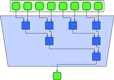
Figure 3.9 Tree reduction pattern. This diagram shows a tree ordering that has a span of lg n, so a speedup of n/lg n is possible. Assuming the combiner function is associative, this ordering computes the same result as Figure 3.8 and Listing 3.9.
There are some variants of this pattern that arise from combination with partition and search such as the category reduction pattern discussed in Section 3.6.8.
Applications of reduction are diverse, and include averaging of Monte Carlo (random) samples for integration; convergence testing in iterative solution of systems of linear equations, such as conjugate gradient; image comparison metrics as in video encoding; and dot products and row–column products in matrix multiplication. Reductions can also use operations other than addition, such as maximum, minimum, multiplication, and Boolean AND, OR, and XOR, and these also have numerous applications. However, you should be cautious of operations that are not truly associative, such as floating point addition. In these cases, different orderings can give different results; this is discussed further in Chapter 5.
3.3.5 Scan
Scan computes all partial reductions of a collection. In other words, for every output position, a reduction of the input up to that point is computed. Serial code implementing scan is shown in Listing 3.10. The ordering used in this code corresponds to Figure 3.10. Scan, and in particular the code shown in Listing 3.10, is not obviously parallelizable since each iteration of the loop depends on the output of the previous iteration. In general, scan is a special case of a serial pattern called a fold. In a fold, a successor function f is used to advance from the previous state to the current state, given some additional input. If the successor function is not associative we cannot, in fact, generally parallelize a fold. However, if the successor function is associative, we can reorder operations (and possibly add some extra work) to reduce the span and allow for a parallel implementation. Associativity of the successor function is what distinguishes the special case of a scan from the general case of a fold. A parallelizable scan can be used in this example because the successor function is addition, which is associative.
Listing 3.10 Serial implementation of scan.
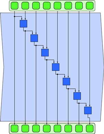
Figure 3.10 Serial scan pattern. This is one way of many possible to implement scan, but has a span of order Θ(n) and so is not parallelizable. This implementation of scan corresponds to the code in Listing 3.10.
One possible parallel implementation of scan when the successor function f is associative is shown in Figure 3.11. As you can see, parallelization of scan is less obvious than parallelization of reduction. We will consider various implementation alternatives in Section 5.4, but if the programming model supports scan as a built-in operation it may not be necessary to consider the details of the implementation.
Figure 3.11 Parallel scan pattern. If the successor function is associative, many reorderings are possible with lower span. This is one of many possible ways to implement scan using a span of order Θ(lg n). It consists basically of a reduction tree followed by some additional operations to compute additional intermediate partial reductions not computed by the tree. Notice, however, that the total amount of work is more than the algorithm used in Figure 3.10.
However, it is worth noting that a parallel implementation of scan may require more work (evaluations of f) than is necessary in the serial case, up to twice as many, and also at best only has Θ(lg n) span. Scan is a good example of an algorithm that is parallelizable but for which linear speedup is not possible and for which the parallel algorithm is not as efficient in terms of the total number of operations required as the serial implementation. Because of this, use of scan can limit scaling and alternative algorithms should be considered whenever possible.
Examples of the use of the scan pattern include integration, sequential decision simulations in option pricing, and random number generation. However, use of scan in random number generation is only necessary if one is forced to parallelize traditional sequential pseudorandom number generators, which are often based on successor functions. There are alternative approaches to pseudorandom number generation based on hashing that require only the map pattern [SMDS11]. For greater scalability, these should be used when possible.
Scan can also be used to implement pack in combination with scatter, but a pack operation is intrinsically deterministic, unlike scatter. Therefore, we have included pack as a separate pattern.
3.3.6 Recurrence
The map pattern results when we parallelize a loop where the loop bodies are all independent. A recurrence is also a generalization of iteration, but of the more complex case where loop iterations can depend on one another. We consider only simple recurrences where the offsets between elements are constant. In this case, recurrences look somewhat like stencils, but where the neighbor accesses can be to both inputs and outputs. A recurrence is like a map but where elements can use the outputs of adjacent elements as inputs.
There is a constraint that allows recurrences to be computable: They must be causal. That is, there must be a serial ordering of the recurrence elements so that elements can be computed using previously computed outputs. For recurrences that arise from loop nests, where output dependencies are really references to values computed in previous loop iterations, a causal order is given. In fact, it turns out that there are two cases where recurrences are parallelizable: (1) a 1D recurrence where the computation in the element is associative, (2) and a multidimensional recurrence arising from a nested loop body. The 1D case we have already seen: It is just the scan pattern in Section 3.3.5. In the nD case arising from nested loops, surprisingly, recurrences are always parallelizable over n − 1 dimensions by sweeping a hyperplane over the grid of dependencies [Lam74], an approach discussed in Section 7.5. This can be implemented using a sequence of stencils. Conversely, iterated stencils can be reinterpreted as recurrences over space–time.
Recurrences arise in many applications including matrix factorization, image processing, PDE solvers, and sequence alignment. Partial differentiation equation (PDE) solvers using iterated stencils, such as the one discussed in Chapter 10, are often converted into space–time recurrences to apply space–time tiling. Space–time tiling is an optimization technique for recurrences discussed in Section 7.5. Using this optimization can be more efficient than treating the stencil and the iteration separately, but it does require computing several iterations at once.
3.4 Serial Data Management Patterns
Data can be managed in various ways in serial programs. Data management includes how storage of data is allocated and shared as well as how it is read, written, and copied.
3.4.1 Random Read and Write
The simplest mechanism for managing data just relies directly on the underlying machine model, which supplies a set of memory locations indexed by integers (“addresses”). Addresses can be represented in higher-level programming languages using pointers.
Unfortunately, pointers can introduce all kinds of problems when a program is parallelized. For example, it is often unclear whether two pointers refer to the same object or not, a problem known as aliasing. In Listing 3.8, we show how this can happen when variables are passed as function arguments. Aliasing can make vectorization and parallelization difficult, since straightforward approaches will often fail if inputs are aliased. On the other hand, vectorization approaches that are safe in the presence of aliasing may require extra data copies and may be considered unacceptably expensive. A common approach is to forbid aliasing or to state that vectorized functions will have undefined results if inputs are aliased. This puts the burden on the programmer to ensure that aliases do not occur.
Array indices are a slightly safer abstraction that still supports data structures based on indirection. Array indices are related to pointers; specifically, they represent offsets from some base address. However, since array indices are restricted to the context of a particular collection of data they are slightly safer. It is still possible to have aliases but at least the range of memory is restricted when you use array indices rather than pointers. The other advantage of using array indices instead of pointers is that such data structures can be easily moved to another address space, such as on a co-processor. Data structures using raw pointers are tied to a particular address space.
3.4.2 Stack Allocation
Frequently, storage space for data needs to be allocated dynamically. If data is allocated in a nested last in, first out (LIFO) fashion, such as local variables in function calls, then it can be allocated on a stack. Not only is stack allocation efficient, since an arbitrary amount of data can be allocated in constant time, but it is also locality preserving.
To parallelize this pattern, typically each thread of control will get its own stack so locality is preserved. The function-calling conventions of Cilk Plus generalize stack allocation in the context of function calls so the locality preserving properties of stack allocation are retained.
3.4.3 Heap Allocation
In many situations, it is not possible to allocate data in a LIFO fashion with a stack. In this case, data is dynamically allocated from a pool of memory commonly called the heap. Heap allocation is considerably slower and more complex than stack allocation and may also result in allocations scattered all over memory. Such scattered allocations can lead to a loss in coherence and a reduction in memory access efficiency. Widely separated accesses are more expensive than contiguous allocations due to memory subsystem components that make locality assumptions, including caches, memory banks, and page tables. Depending on the algorithm used, heap allocation of large blocks of different sizes can also lead to fragmented memory [WJNB95]. When memory is fragmented, contiguous regions of address space may not be available even though enough unallocated memory is available in total. Fragmentation is less of a problem on machines with virtual memory because only the memory addresses actually in use will occupy physical memory, at least at the granularity of a page.
When parallelizing programs that use heap allocation, you should be aware that implicitly sharing the data structure used to manage the heap can lead to scalability problems. A parallelized heap allocator should be used when writing parallel programs that use dynamic memory allocation. Such an allocator maintains separate memory pools on each worker, avoiding constant access to global locks. Such a parallelized allocator is provided by TBB and can be used even if the other constructs of TBB are not.
For efficiency, many programs use simple custom allocators rather than the more general heap. For example, to manage the allocation of items that are all the same size, free items can be stored on a linked list and allocated in constant time. This also has the advantage of reducing fragmentation since elements of the same size are allocated from the same pool. However, if you implement your own allocation data structures, when the code is parallelized even a simple construct like a linked list can become a bottleneck if protected with a lock. Conversely, if it is not protected, it can be a race condition hazard.
3.4.4 Closures
Closures are function objects that can be constructed and managed like data. Lambda functions (see Appendix D.2) are simply unnamed closures that allow functions to be syntactically defined where and when needed. As we will see, the new C++ standard includes lambda functions that are used extensively by TBB. ArBB also allows closure objects to be constructed and compiled dynamically but does not require that lambda functions be supported by the compiler.
When closures are built, they can often be used to “capture” the state of non-local variables that they reference. This implicitly requires the use of dynamic memory allocation. Closures can also be generated dynamically or statically. If they are statically implemented, then the implementation may need to allow for a level of indirection so the code can access the data associated with the closure at the point it is created. If the code for the closure is dynamically constructed, as in ArBB, then it is possible to use the state of captured variables at the point of construction to optimize the generated code.
3.4.5 Objects
Objects are a language construct that associate data with the code to act on and manage that data. Multiple functions may be associated with an object and these functions are called the methods or member functions of that object. Objects are considered to be members of a class of objects, and classes can be arranged in a hierarchy in which subclasses inherit and extend the features of superclasses. All instances of a class have the same methods but have different state. The state of an object may or may not be directly accessible; in many cases, access to an object’s state may only be permitted through its methods.
In some languages, including C++, subclasses can override member functions in superclasses. Overriding usually requires class and function pointers in the implementation, but function pointers in particular may not be supported on all hardware targets (specifically older GPUs). Some programming models, such as ArBB, partially avoid this problem by providing an additional stage of compilation at which the function pointers can be resolved so they do not have to be resolved dynamically during execution.
In parallel programming models objects have been generalized in various ways. For example, in Java, marking a method as synchronized adds a lock that protects an object’s state from being modified by multiple methods at once. However, as discussed in Section 2.6.2, overuse of locks can be detrimental to performance.
Closures and objects are closely related. Objects can be fully emulated using just closures, for example, and the implementation of objects in Smalltalk [Kay96] was inspired in part by the implementation of nested functions in Algol and Simula [Per81, Nau81, Coh96].
3.5 Parallel Data Management Patterns
Several patterns are used to organize parallel access to data. In order to avoid problems such as race conditions, it is necessary in parallel programs to understand when data is potentially shared by multiple workers and when it is not. It is especially important to know when and how multiple workers can modify the same data. For the most part the parallel data access patterns we will discuss in this book avoid modification of shared data or only allow its modification in a structured fashion. The exception is the scatter pattern, several variants of which can still be used to resolve or avoid race conditions. Some of these patterns are also important for data locality optimizations, such as partition, although these also have the affect of creating independent regions of memory that can safely be modified in parallel.
3.5.1 Pack
The pack pattern can be used to eliminate unused space in a collection. Elements of a collection are each marked with a Boolean value. Pack discards elements in the data collection that are marked with false. The remaining elements marked with true are placed together in a contiguous sequence, in the same order they appeared in the input data collection. This can be done either for each element of the output of a map or in a collective fashion, using a collection of Booleans that is the same shape as the data collection and is provided as an additional input. See Figure 3.12 for an illustration of the pack pattern with a specific set of input data.
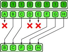
Figure 3.12 Pack pattern. Unused elements are discarded and the remainder packed together in a contiguous sequence.
Pack is especially useful when fused with map and other patterns to avoid unnecessary output from those patterns. When properly implemented, a programming system can use pack to reduce memory bandwidth. Pack can even be used as a way to emulate control flow on SIMD machines with good asymptotic performance [LLM08, HLJH09], unlike the masking approach.
An inverse of the pack operation, unpack, is also useful. The unpack operation can place elements back into a data collection at the same locations from which they were drawn with a pack. Both pack and unpack are deterministic operations. Pack can also be implemented using a combination of scan and scatter [Ble93].
Examples of the use of pack include narrow-phase collision detection pair testing when you only want to report valid collisions and peak detection for template matching in computer vision.
3.5.2 Pipeline
A pipeline pattern connects tasks in a producer–consumer relationship. Conceptually, all stages of the pipeline are active at once, and each stage can maintain state that can be updated as data flows through them. See Figure 3.13 for an example of a pipeline. A linear pipeline is the basic pattern but more generally, a set of stages could be assembled in a directed acyclic graph. It is also possible to have parallel stages, as will be discussed in Chapter 9.
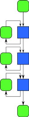
Figure 3.13 Pipeline pattern. Stages are connected in a producer–consumer relationship, and each stage can maintain state so that later outputs can depend on earlier ones.
Pipelines are useful for serially dependent tasks like codecs for encoding and decoding video and audio streams. Stages of the pipeline can often be generated by using functional decomposition of tasks in an application. However, typically this approach results in a fixed number of stages, so pipelines are generally not arbitrarily scalable. Still, pipelines are useful when composed with other patterns since they can provide a multiplier on the available parallelism.
Examples of the use of the pipeline pattern include codecs with variable-rate compression, video processing and compositioning systems, and spam filtering.
3.5.3 Geometric Decomposition
The geometric decomposition pattern breaks data into a set of subcollections. In general these subcollections can overlap. See the middle example in Figure 3.14. If the outputs are partitioned into non-overlapping domains, then parallel tasks can operate on each subdomain independently without fear of interfering with others. See the rightmost example in Figure 3.14. We will call the special case of non-overlapping subregions the partition pattern.
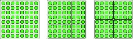
Figure 3.14 Geometric decomposition and the partition pattern. In the geometric decomposition pattern, the data is divided into potentially overlapping regions (middle, four 5 × 5 regions). The partition pattern is a special case of geometric decomposition where the domain is divided into non-overlapping regions (right, four 4 × 4 regions).
The partition pattern is very useful for divide-and-conquer algorithms, and it can also be used in efficient parallel implementations of the stencil pattern. For the stencil pattern, typically the input is divided into a set of partially overlapping strips (a general geometric decomposition) so that neighbors can be accessed. However, the output is divided into non-overlapping strips (that is, a partition) so that outputs can be safely written independently. Generally speaking, if overlapping regions are used they should be for input, while output should be partitioned into non-overlapping regions.
An issue that arises with geometric decomposition is how boundary conditions are handled when the input or output domains are not evenly divisible into tiles of a consistent size.
A geometric decomposition does not necessarily move data. It often just provides an alternative “view” of the organization. In the special case of the partition pattern, a geometric decomposition makes sure that different tasks are modifying disjoint regions of the output.
We have shown diagrams where the data is regularly arranged in an array and the decomposition uses regular subarrays. It would also be possible to have subcollections of different sizes, or for subcollections to be interleaved (for example, all the odd elements in one subcollection and all the even ones in the other). It is also possible to apply this pattern to less regular data structures, such as graphs. For example, a graph coloring might be used to divide the vertices of a graph into a subset of vertices that are not directly connected, or a graph might be divided into components in other ways.
The implementation of stencil operations, which are used in both image processing and simulation, are a good example of the use of geometric decomposition with overlapping input regions. When iterated stencils are implemented on distributed memory computers such as clusters, often one subdomain is assigned to each processor, and then communication is limited to only the overlap regions. Examples of the use of partition (with non-overlapping regions) include JPEG and other macroblock compression, as well as divide-and-conquer matrix multiplication.
3.5.4 Gather
The gather pattern reads a collection of data from another data collection, given a collection of indices. Gather can be considered a combination of map and random serial read operations. See Figure 3.15 for an example. The element type of the output collection is the same as the input data collection but the shape of the output collection is that of the index collection. Various optimizations are possible if the array of indices is fixed at code generation time or follows specific known patterns. For example, shifting data left or right in an array is a special case of gather that is highly coherent and can be accelerated using vector operations. The stencil pattern also performs a coherent form of gather in each element of a map, and there are specific optimizations associated with the implementation of such structured, local gathers.
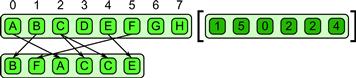
Figure 3.15 Gather pattern. A collection of data is read from an input collection given a collection of indices.
Examples of gather include sparse matrix operations, ray tracing, volume rendering, proximity queries, and collision detection.
3.5.5 Scatter
The scatter pattern is the inverse of the gather pattern: A set of input data and a set of indices is given, but each element of the input is written at the given location, not read. The scatter can be considered equivalent to a combination of the map and random serial write patterns. Figure 3.16 illustrates a problem with scatter, however: What do we do if two writes go to the same location?
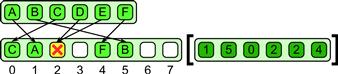
Figure 3.16 Scatter pattern. A collection of data is written to locations given by a collection of addresses. However, what do we do when two addresses are the same?
Unfortunately, in the naïve definition of scatter, race conditions are possible when there are duplicate write addresses. In general, we cannot even assume that either value is written properly. We will call such duplicates collisions. To obtain a full definition of scatter, we need to define what to do when such collisions occur. To obtain a deterministic scatter, we need rules to deterministically resolve collisions.
There are several possible solutions to the problem of collisions, including using associative operators to combine values, choosing one of the multiple values non-deterministically, and assigning priorities to values. These will be discussed in detail in Section 6.2.
3.6 Other Parallel Patterns
In this section we will discuss several additional patterns that often show up in practice, but for which we unfortunately do not have any specific code examples in this book. Please check online, as more details and examples for these patterns may be available there. Some of these patterns are extensions or elaborations of already discussed patterns.
3.6.1 Superscalar Sequences
In the superscalar sequence pattern, you write a sequence of tasks, just as you would for an ordinary serial sequence. As an example, consider the code shown in Listing 3.11. However, unlike the case with the sequence pattern, in a superscalar sequence tasks only need to be ordered by data dependencies [ERB+10, TBRG10, KLDB10]. As long as there are no side effects, the system is free to execute tasks in parallel or in a different order than given in the source code. As long as the data dependencies are satisfied, the result will be the same as if the tasks executed in the canonical order given by the source code. See Figure 3.17.
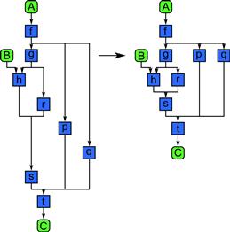
Figure 3.17 Superscalar sequence pattern. A superscalar sequence orders operations by their data dependencies only. On the left we see the timing given by a serial implementation of the code in Listing 3.11 using the sequence pattern. However, if we interpret this graph as a superscalar sequence, we can potentially execute some of the tasks simultaneously, as in the diagram on the right. Tasks in a superscalar sequence must not have any hidden data dependencies or side-effects not known to the scheduler.
The catch here is the phrase “as long as the data dependencies are satisfied.– In order to use this pattern, all dependencies need to be visible to the task scheduler.
This pattern is related to futures, discussed in Section 3.6.2. However, unlike with futures, for superscalar sequences you do not explicitly manage or wait on parallel tasks. Superscalar sequences are meant to be serially consistent.
3.6.2 Futures
The futures pattern is like fork–join, but the tasks do not have to be nested hierarchically. Instead, when a task is spawned, an object is returned—a future—which is used to manage the task. The most important operation that can be done on a future is to wait for it to complete. Futures can implement the same hierarchical patterns as in fork–join but can also be used to implement more general, and potentially confusing, task graphs. Conceptually, fork–join is like stack-based allocation of tasks, while futures are like heap allocation of tasks.
Listing 3.11 Superscalar sequence in pseudocode.
Task cancellation can also be implemented on futures. Cancellation can be used to implement other patterns, such as the non-deterministic branch-and-bound pattern or speculative selection.
3.6.3 Speculative Selection
Speculative selection generalizes selection so that the condition and both alternatives can run in parallel. Compare Figure 3.4 with Figure 3.18. When the condition completes, the unneeded branch of the speculative selection is cancelled. Cancellation also needs to include the reversal of any side-effects. In practice, the two branches will have to block at some point and wait for the condition to be evaluated before they can commit any changes to state or cause any non-reversible side-effects. This pattern is inherently wasteful, as it executes computations that will be discarded. This means that it always increases the total amount of work.
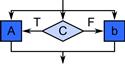
Figure 3.18 Speculative selection pattern. The speculative selection pattern is like the serial selection pattern, but we can start the condition evaluation and both sides of the selection at the same time. When the condition is finished evaluating, the unneeded branch is “cancelled.”
It can be expensive to implement cancellation, especially if we have to worry about delaying changes to memory or side-effects. To implement this pattern, the underlying programming model needs to support task cancellation. Fortunately, TBB does support explicit task cancellation and so can be used to implement this pattern.
Speculative selection is frequently used at the very finest scale of parallelism in compilers for hiding instruction latency and for the simulation of multiple threads on SIMD machines.
In the first case, instructions have a certain number of cycles of latency before their results are available. While the processor is executing the instructions for the condition in an if statement, we might as well proceed with the first few instructions of one of the branches. In this case, the speculation pattern might not actually be wasteful, since those instruction slots would have otherwise been idle; however, we do not want to commit the results. Once we know the results of the condition, we may have to discard the results of these speculatively executed instructions. You rarely have to worry about the fine-scale use of this pattern, since it is typically implemented by the compiler or even the hardware. In particular, out-of-order hardware makes extensive use of this pattern for higher performance, but at some cost in power.
However, in the SIMT machine model, multiple threads of control flow are emulated on SIMD machines using masking, which is related to speculative selection. In order to emulate if statements in this model, the condition and both the true and false branches are all evaluated. However, the memory state is updated using masked memory writes so that the results of executing the true branch are only effective for the lanes where the condition was true and conversely for the false branch. This can be optimized if we find the condition is all true or all false early enough, but, like speculative selection, SIMT emulation of control flow is potentially wasteful since results are computed that are not used. Unlike the case with filling in unused instruction slots, using masking to emulate selection like this increases the total execution time, which is the sum of both branches, in addition to increasing the total amount of work.
A similar approach can also be used to emulate iteration on SIMD machines, but in the case of iteration the test for all-true or all-false is used to terminate the loop. In both cases, we may only use the SIMD model over small blocks of a larger workload and use a threading model to manage the blocks.
3.6.4 Workpile
The workpile pattern is a generalization of the map pattern where each instance of the elemental function can generate more instances and add them to the “pile” of work to be done. This can be used, for example, in a recursive tree search, where we might want to generate instances to process each of the children of each node of the tree.
Unlike the case with the map pattern with the workpile pattern the total number of instances of the elemental function is not known in advance, nor is the structure of the work regular. This makes the workpile pattern harder to vectorize than the map pattern.
3.6.5 Search
Given a collection, the search pattern finds data that meets some criteria. The criteria can be simple, as in an associative array, where typically the criteria is an exact match with some key. The criteria can also be more complex, such as searching for a set of elements in a collection that satisfy a set of logical and arithmetic constraints.
Searching is often associated with sorting, since to make searches more efficient we may want to maintain the data in sorted order. However, this is not necessarily how efficient searches need to be implemented.
Searching can be very powerful, and the relational database access language, SQL, can be considered a data-parallel programming model. The parallel embedded language LINQ from Microsoft uses generalized searches as the basis of its programming model.
3.6.6 Segmentation
Operations on collections can be generalized to operate on segmented collections. Segmented collections are 1D arrays that are subdivided into non-overlapping but non-uniformly sized partitions. Operations such as scan and reduce can then be generalized to operate on each segment separately, and map can also be generalized to operate on each segment as a whole (map-over-segments) or on every element as usual. Although the lengths of segments can be non-uniform, segmented scans and reductions can be implemented in a regular fashion that is independent of the distribution of the lengths of the segments [BHC+93]. Segmented collective operations are more expensive than regular reduction and scan but are still easy to load balance and vectorize.
The segmentation pattern is interesting because it has been demonstrated that certain recursive algorithms, such as quicksort [Ble90, Ble96], can be implemented using segmented collections to operate in a breadth-first fashion. Such an implementation has advantages over the more obvious depth-first parallel implementation because it is more regular and so can be vectorized. Segmented operations also arise in time-series analysis when the input data is segmented for some reason. This frequently occurs in financial, vision, and speech applications when the data is in fact segmented, such as into different objects or phonemes.
3.6.7 Expand
The expand pattern can be thought of as the pack pattern merged with map in that each element of a map can selectively output elements. However, in the expand pattern, each element of the map can output any number of elements—including zero. The elements are packed into the output collection in the order in which they are produced by each element of the map and in segments that are ordered by the spatial position of the map element that produced them. An example is shown in Figure 3.19.
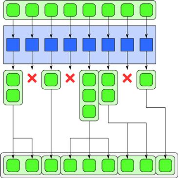
Figure 3.19 Expand pattern. Each element of a map can output zero or more elements, which are packed in the order produced and organized into segments corresponding to the location of the elements in the map that produced them.
Examples of the use of expand include broad-phase collision detection pair testing when reporting potentially colliding pairs, and compression and decompression algorithms that use variable-rate output on individually compressed blocks.
3.6.8 Category Reduction
Given a collection of data elements each with an associated label, the category reduction pattern finds all elements with the same label and reduces them to a single element using an associative (and possibly commutative) operator. The category reduction pattern can be considered a combination of search and segmented reduction. An example is provided in Figure 3.20.
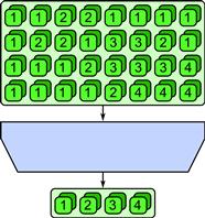
Figure 3.20 Category reduction pattern. Given an input collection with labels, all elements with the same label are collected and then reduced to a single element.
Searching and matching are fundamental capabilities and may depend indirectly on sorting or hashing, which are relatively hard to parallelize. This operation may seem esoteric, but we mention it because it is the form of “reduction” use in the Hadoop [Kon11, DG04] Map-Reduce programming model used by Google and others for highly scalable distributed parallel computation. In this model, a map generates output data and a set of labels, and a category reduction combines and organizes the output from the map. It should be emphasized that they do not call the reduction used in their model a category reduction. However, we apply that label to this pattern to avoid confusion with the more basic reduction pattern used in this book.
Examples of use of category reduction include computation of metrics on segmented regions in vision, computation of web analytics, and thousands of other applications implemented with Map-Reduce.
3.6.9 Term Graph Rewriting
In this book we have primarily focused on parallel patterns for imperative languages, especially C++. However, there is one very interesting pattern that is worth mentioning due to its utility in the implementation of functional languages: term graph rewriting.
Term graph rewriting matches patterns in a directed acyclic graph, specifically “terms” given by a head node and a sequence of children. It then replaces these terms with new subgraphs. This is applied over and over again, evolving the graph from some initial state to some final state, until no more substitutions are possible. It is worth noting that in this book we have used graphs to describe the relationships between tasks and data. However, in term graph rewriting, graphs are the data, and it is the evolution of these graphs over time that produces the computation.
Term graph rewriting is equivalent in power to the lambda calculus, which is usually used to define the semantics of functional languages. However, term graph rewriting is more explicit about data sharing since this is expressed directly in the graph, and this is important for reasoning about the memory usage of a functional program. Term graph rewriting can take place in parallel in different parts of the graph, since under some well-defined conditions term graph rewriting is confluent: It does not matter in which order the rewrites are done; the same result will be produced either way. A very interesting parallel functional language called Concurrent Clean has been implemented using this idea [PvE93, PvE99]. Many other parallel languages, including hardware simulation and synthesis languages, have been defined in terms of this pattern.
3.7 Non-Deterministic Patterns
Normally it is desirable to avoid non-determinism since it makes testing and debugging much more difficult. However, there are some potentially useful non-deterministic patterns.
We will discuss two non-deterministic patterns in this section, branch and bound and transactions. In some cases, such as search, the input–output behavior of the abstraction may be deterministic but the implementation may be non-deterministic internally. It is useful to understand when non-determinism can be contained inside some abstraction, and conversely when it affects the entire program.
3.7.1 Branch and Bound
The branch and bound pattern is often used to implement search, where it is highly effective. It is, however, a non-deterministic pattern and a good example of when non-determinism can be useful.
Suppose you have a set of items and you want to do an associative search over this set to find an item that matches some criteria. To do a parallel search, the simplest approach is to partition the set and search each subset in parallel. However, suppose we only need one result, and any data that satisfies the search criteria is acceptable. In that case, once an item matching the search criteria is found, in any one of the parallel subset searches, the searches in the other subsets can be cancelled.
The branch and bound strategy can actually lead to superlinear speedups, unlike many other parallel algorithms. However, if there are multiple possible matches, this pattern is non-deterministic because which match is returned depends on the timing of the searches over each subset. Since this form of non-determinism is fundamental in the definition of the result (“return the first result found that matches the criteria”), it is hard to remove this form of non-determinism. However, to get a superlinear speedup, the cancellation of in-progress tasks needs to be implemented in an efficient manner.
This pattern is also used for mathematical optimization, but with a few additional features. In mathematical optimization, you are given an objective function, some constraint equations, and a domain. The function depends on certain parameters. The domain and the constraint equations define legal values for the parameters. Within the given domain, the goal of optimization is to find values of the parameters that maximize (or minimize) the objective function.
Search and optimization are related in that in optimization we are searching for the location of the optimum, so one way to approach the problem is exactly like with search: Break up the domain into subdomains, search each region in parallel, and when a “good enough” value is found in one domain cancel the other parallel searches. But what conditions, exactly, allow us to cancel other searches? We can cancel a search if we can prove that the optimum in a domain Y can be no better than y but we have already found a solution x better than y. In this case we can cancel any search in Y. Mathematically, we can compute bounds using techniques such as interval analysis [HW04] and often apply the subdivide-and-bound approach recursively.
What is interesting about this is that the global optima are fixed by the mathematical problem; therefore, they are unique. The code can be designed to return the same result every time it is run. Even though the algorithm might be non-deterministic internally, the output can be deterministic if implemented carefully.
The name “branch and bound” comes from the fact that we recursively divide the problem into parts, then bound the solution in each part. Related techniques, such as alpha-beta pruning [GC94], are also used in state-space search in artificial intelligence.
3.7.2 Transactions
Transactions are used when a central repository for data needs several different updates and we do not care what order the updates are done in, as long as the repository is kept in a consistent state. An example would be a database recording transactions on a bank account. We do not care too much in what order the deposits and withdrawals are recorded, as long as the balance at the end of the day is correct. In fact, in this special case, since deposits and withdrawals are using an associative operation (addition), the result is in fact deterministic. However, in general, transaction operations will be non-associative and in that case the outcome will not be deterministic if the order in which the individual operations are performed is non-deterministic.
For a concrete example that illuminates where transactions might be useful, suppose you are using a hash table. The kinds of operations you want to use on a hash table might involve inserting elements and searching for elements. Suppose that the hash table is implemented using a set of buckets with elements that map to the same bucket stored in a linked list. If multiple parallel tasks try to insert elements into the same bucket, we could use some implementation of the transaction pattern to make sure the linked lists are updated consistently. The order in which the elements are inserted into the linked lists may not be consistent from run to run. However, the overall program may still be deterministic if the internal non-determinism is not exposed outside the implementation of the pattern itself—that is, if hash table searches always return the same data no matter what the initial ordering of the lists was.
Implementing a deterministic hash table using non-deterministic mechanisms may require some additional effort, however. For example, suppose the same key is inserted twice with different data. In this case, suppose only one of the two possible data elements should be retained. If we retain the last element inserted, creating a dependency on timing, the hash table will be non-deterministic and this has the potential to make the whole program non-deterministic. On the other hand, if we use a rule to choose which of the two data elements to retain, such as picking the largest data element, then we can make the output deterministic.
The implementation of transactions is important. Of course, they could be implemented with locks, but a more scalable approach uses a commit and rollback protocol, as in a database transactions. When the term “transactions” is used it generally refers to this form of implementation.
3.8 Programming Model Support for Patterns
Many of the patterns discussed in this chapter are supported directly in one or more of the programming models discussed in this book. By direct support, we mean that there is a language construct that corresponds to the pattern. Even if a pattern is not directly supported by one of the programming models we consider, it may be possible to implement it using other features.
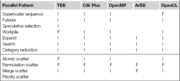
In the following, we briefly describe the patterns supported by each of Cilk Plus, TBB, OpenMP, ArBB, and OpenCL. Patterns can be supported directly by a feature of the programming model, or they may be implementable using other features. A summary of serial pattern support is provided in Table 3.1, and a summary of parallel pattern support is provided in Tables 3.2 and 3.3. These tables use an F to indicate when a programming model includes an explicit feature supporting that pattern, an I if the pattern is implementable with that model, or a blank if there is no straightforward way to implement the pattern with that model. Some patterns are implementable with other patterns, and when an example of this is given in the book it is indicated with a P. Table 3.2 also includes section references to examples using or implementing that pattern. Table 3.3 indicates support for some additional patterns that are discussed in this book but for which, unfortunately, no suitable examples were available.
Table 3.1. Summary of programming model support for the serial patterns discussed in this book. Note that some of the parallel programming models we consider do not, in fact, support all the common serial programming patterns. In particular, note that recursion and memory allocation are limited on some model.
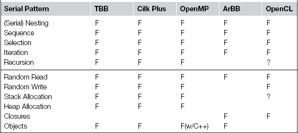
Table 3.2. Summary of programming model support for the patterns discussed in this book. F: Supported directly, with a special feature. I: Can be implemented easily and efficiently using other features. P: Implementations of one pattern in terms of others, listed under the pattern being implemented. Blank means the particular pattern cannot be implemented in that programming model (or that an efficient implementation cannot be implemented easily). When examples exist in this book of a particular pattern with a particular model, section references are given.
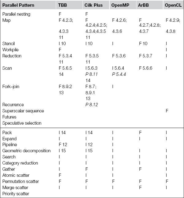
Table 3.3. Additional patterns discussed. F: Supported directly, with a special feature. I: Can be implemented easily and efficiently using other features. Blank means the particular pattern cannot be implemented in that programming model (or that an efficient implementation cannot be implemented easily).
We additionally provide section references when an example is given in this book of a particular parallel pattern with a particular model. Unfortunately space does not permit us to give an example of every parallel pattern with every programming model, even when a pattern is implementable with that model. In other cases, common patterns (such as map) may show up in many different examples. Please refer to the online site for the book. Some additional examples will be made available there that can fill in some of these gaps.
3.8.1 Cilk Plus
The feature set of Cilk Plus is simple, based primarily on an efficient implementation of the fork–join pattern, but general enough that many other patterns can also be implemented in terms of its basic features. Cilk Plus also supports many of the other patterns discussed in this chapter as built-in features, with implementations usually built around fork–join. For some patterns, however, it may be necessary to combine Cilk Plus with components of TBB, such as if atomic operations or scalable parallel dynamic memory allocation are required. Here are the patterns supported directly by Cilk Plus.
Nesting, Recursion, Fork–Join
Nesting to arbitrary depth is supported by cilk_spawn. Specifically, this construct supports fork–join parallelism, which generalizes recursion. Support for other patterns in Cilk Plus are based on this fundamental mechanism and so can also be nested. As discussed later, fork–join in Cilk Plus is implemented in such a way that large amounts of parallel slack(the amount of potential parallelism) can be expressed easily but can be mapped efficiently (and mostly automatically) onto finite hardware resources. Specifically, the cilk_spawn keyword only marks opportunities for a parallel fork; it does not mandate it. Such forks only result in parallel execution if some other core becomes idle and looks for work to “steal.”
Reduction
The reduction pattern is supported in a very general way by hyperobjects in Cilk Plus. Hyperobjects can support reductions based on arbitrary commutative and associative operations. The semantics of reduction hyperobjects are integrated with the fork–join model: new temporary accumulators are created at spawn points, and the associative combiner operations are applied at joins.
Map, Workpile
The map pattern can be expressed in Cilk Plus using cilk_for. Although a loop syntax is used, not all loops can be parallelized by converting them to cilk_for, since loops must not have loop-carried dependencies. Only loops with independent bodies can be parallelized, so this construct is in fact a map. This is not an uncommon constraint in programming models supporting “parallel for” constructs; it is also true of the “for” constructs in TBB and OpenMP. The implementation of this construct in Cilk Plus is based on recursive subdivision and fork–join, and so distributes the overhead of managing the map over multiple threads.
The map pattern can also be expressed in Cilk Plus using elemental functions, which when invoked inside an explicitly vectorized loop also give a “map” pattern. This form explicitly targets vector instructions. Because of this, it is more constrained than the cilk_for mechanism. However, these mechanisms can be composed.
The workpile pattern can be implemented in Cilk Plus directly on top of the basic fork–join model.
Scatter, Gather
The Cilk Plus array notations support scatter and gather patterns directly. The array notations also allow sequences of primitive map operations (for example, the addition of two arrays) to be expressed. Operations on entire arrays are supported with a special array slice syntax.
3.8.2 Threading Building Blocks
Threading Building Blocks (TBB) supports fork–join with a work-stealing load balancer as its basic model. In contrast with Cilk Plus, TBB is a portable ISO C++ library, not a compiler extension. Because TBB is not integrated into the compiler, its fork–join implementation is not quite as efficient as Cilk Plus, and it cannot directly generate vectorized code. However, TBB also provides implementations of several patterns not available directly in Cilk Plus, such as pipelines. Because it is a portable library, TBB is also available today for more platforms than Cilk Plus, although this may change over time.
In addition to a basic work-stealing scheduler that supports the fork–join model of parallelism, TBB also includes several other components useful in conjunction with other programming models, including a scalable parallel dynamic memory allocator and an operating-system-independent interface for atomic operations and locks. As previously discussed, locks should be used with caution and as a last resort, since they are non-deterministic and can potentially cause deadlocks and race conditions. Locks also make scheduling non-greedy, which results in sub-optimal scheduling. Here are the patterns supported directly by TBB.
Nesting, Recursion, Fork–Join
TBB supports nesting of tasks to arbitrary depth via the fork–join model. Like Cilk Plus, TBB uses work-stealing load balancing which is both scalable and locality-preserving. However, TBB can also support more general task graph dependencies than the planar graphs generated by the Cilk Plus fork–join implementation. These patterns are accessed by the parallel_invoke and task graph features of TBB.
Map
The map patterns is implemented in TBB using the parallel_for and parallel_foreach functions. Lambda functions can be used as arguments to these so that the required elemental function can be described as part of the call rather than being separately declared. As is clear from the names, these functions are useful for parallelizing for loops, but they do have some additional restrictions, so not all for loops can be parallelized. In particular, each invocation of the elemental function body needs to be independent, as we have described for the map pattern, and the number of iterations needs to be fixed and known in advance.
Workpile
The workpile pattern can be accessed from TBB using the parallel_do construct. This is similar to the parallel_for pattern, with the difference that the number of invocations does not need to be known in advance. In fact, additional invocations can be generated from inside the “body” of this construct.
Reduction
The reduction pattern can be accessed via the parallel_reduce construct. This construct allows the specification of an arbitrary combiner function. However, in order for the result to be computed deterministically the reduction function needs to be both associative and commutative (not just associative). If a deterministic reduction is needed, a deterministic_parallel_reduce function is provided.
Scan
The scan pattern can be accessed via the parallel_scan construct. An arbitrary successor function can be specified in order for the result to be deterministic. As with reduction, such a function must be both fully associative and commutative in order for the scan to be deterministic. There is no built-in deterministic scan in TBB but one can be implemented using other features of TBB.
Pipeline
The pipeline pattern can be specified directly with the parallel_pipeline construct, which can support not only linear pipelines but also directed acyclic graphs of pipeline stages. TBB’s support for pipelines is demonstrated at length in Chapter 9.
Speculative Selection, Branch and Bound
TBB supports task cancellation, which can be used to implement many other patterns, including non-deterministic patterns such as branch and bound.
3.8.3 OpenMP
OpenMP is a standard interface for parallel programming based on annotating serial code so that certain constructs, in particular loops, can be reinterpreted as parallel constructs. The basic patterns it supports directly as features are map and reduce, although other patterns can also be implemented. In addition to the data-parallel map pattern, which also supports vectorization, recent versions of OpenMP also support a general task construct which allows other more irregular patterns to be implemented.
However, the implementation of OpenMP is usually based directly on threads, which raises various practical issues. In particular, nested use of OpenMP can lead to overdecomposition and OpenMP does not include a load balancer. Therefore, nesting is not listed as a pattern supported by OpenMP. Also, certain features in OpenMP that map units of work directly to threads preclude using an automatic task-based load balancer. OpenMP does not include generalized reductions but does include locks. Interestingly, a recent study [AF11] of OpenMP applications showed that the most common use of locks was to implement generalized reductions and load balancing. Inclusion of these features into the OpenMP standard would significantly reduce the need for locks.
One advantage of OpenMP over the other models discussed here is that it is also available for Fortran, as well as C and C++. Cilk Plus is available for both C and C++, while TBB is only available for C++.
Map, Workpile
OpenMP supports the map pattern by annotating a for loop (or DO loop in Fortran) to indicate to the compiler that the annotated loop should be interpreted as a parallel construct. Each iteration of the loop is executed in parallel in a different thread, and the end of the loop body implements a barrier.
The workpile pattern can also be implemented in OpenMP using its task model.
Reduction
When a loop body includes updates to variables declared outside the loop body with a predefined set of associative (or semi-associative floating point) operators, the variable may be marked as a reduction variable. In this case, OpenMP automatically implements a parallel reduction.
Fork–Join
OpenMP supports a general task model that can be used to implement the fork–join pattern. The task model can also be used to implement various other patterns discussed in this book. OpenMP is not a focus of this book, so we do not explore the OpenMP task model in depth, but the addition of tasks adds significant power to the OpenMP programming model.
Stencil, Geometric Decomposition, Gather, Scatter
There is no built-in support for directly expressing stencil, geometric decomposition, gather, or scatter in OpenMP, but many of the applications for which OpenMP is used also use these patterns. However, except for reduction variables, OpenMP generally does not manage data, so data access patterns are expressed through the base language functionality rather than through OpenMP itself.
3.8.4 Array Building Blocks
The basic building blocks of ArBB are based on many of the fundamental patterns discussed in this book. ArBB also supports automatic fusion of these basic building blocks and can generate vectorized code as well as code that runs on multiple cores. Unfortunately, ArBB at present does not support nesting or recursion. The patterns directly supported by ArBB include the following.
Map
The map patterns is supported using elemental functions, which must be separately declared and then invoked by a map operation over a collection or index set. Like the array notation of Cilk Plus, ArBB also supports arithmetic operations over entire collections (in other words, the vector operation style of map) but implements optimizations so that a sequence of such operations is as efficient as a map with an explicit elemental function.
Reduction, Scan
Reductions are supported but only over a set of known operators. Reductions over truly associative operations, such as modular integer addition and minimum and maximum, are both deterministic and repeatable.
The scan pattern is supported with collective operations scan and iscan, again for a fixed set of operators. The scan operation supports both exclusive scan, in which every output does not include the corresponding element of the input, and inclusive scan, in which every output does include the corresponding element of the input.
Although the reduction and scan operations in ArBB do not support custom combiner functions, the ArBB implementation supports automatic fusion of multiple map and reduction operations into a single operation. In practice, this can replace many of the uses of custom reduction and scan functions.
Unfortunately, in the current implementations of reduction and scan in ArBB, the results are not guaranteed to be deterministic if the combiner is not truly associative, in particular for floating-point operations. It is, however, possible to implement deterministic reductions and scans for these operations (as well as for custom combiner functions) using other features of ArBB.
Scatter, Gather
Random reads and writes can be implemented in ArBB using either scalar reads and writes inside maps, or with the collective operations gather and scatter. The scatter implementation only supports the permutation scatter pattern (see Section 6.2), which means it is only guaranteed to work correctly when there are no duplicate addresses. However, duplicates are only checked in a debugging mode. Whenever possible, scatter should be avoided since it is not checked in deployment mode and if used incorrectly could potentially lead to incorrect output.
Pack
The pack pattern is supported directly in ArBB with a collective operation, pack. The inverse of pack is also supported with unpack. Note that pack is a safe, deterministic operation that can be used in place of scatter in many situations.
3.8.5 OpenCL
The OpenCL programming model was designed to allow the use of attached co-processors with separate memories and using a tiled SIMD architecture, such as GPUs, to be accessed as computational devices. It also maps reasonably well onto CPUs with vector instructions.
OpenCL does not support full nesting but does provide two explicit levels of parallelism. One level (work-groups) maps onto the multiple cores in the devices; the other (work-items) maps onto SIMD lanes and hyperthreads in each core.
The programming model of OpenCL is quite similar to that of CUDA, but since OpenCL is standardized and CUDA is not, we only give OpenCL examples in this book.
Map
When a kernel function is written in OpenCL and then executed on a device, it implements the map pattern. This is similar to the use of elemental functions in ArBB and Cilk Plus array notation. Each execution of a kernel executes a set of instances. Each instance is called a work item. When the map is executed, the work items are automatically tiled into sets of parallel work called work groups. Within each work-group, the implementation typically emulates control flow over multiple work items using masking over SIMD lanes. It is also possible to communicate using shared memory within a work group, but not between work groups. Generally, communication requires the insertion of a barrier, since a work group may be further decomposed into multiple chunks by the implementation that may run asynchronously. Barrier-free communication is possible within a single SIMD “chunk” within a work group on specific hardware but this is not standardized, and hence it is not advised.
Gather
Within an OpenCL kernel, random reads to memory can be performed. This can be done either to on-chip local memory (very fast and shared within a work group) or to global memory. On some processors supporting OpenCL, accesses to global memory are cached, but on others they are not. In the latter case, the implementation may use software pipelining to hide memory access latency. Hyperthreads may also be used on multicore processors that support it. The global memory is still typically local to the co-processor, so OpenCL includes additional directives to do memory transfers to and from the host.
Note that with OpenCL maximizing throughput rather than minimizing latency is the goal. Hyperthreads and software pipelining overlap memory access latency with additional computation; they do not eliminate the memory access latency. In fact, use of these techniques can increase latency overall. This style of “throughput” computation may also be used with other throughput-oriented programming models, such as ArBB and CUDA.
Scatter
Scatter is supported in OpenCL but some care is needed to deal with collisions (parallel writes to the same address). Recent versions of OpenCL include standardized atomic operations, and many processors targeted by OpenCL implementations support these efficiently in hardware.
Reduction, Scan, Pack, Expand
OpenCL does not support the reduction pattern directly as a feature but it is implementable. Typically, the array to be reduced is divided into tiles, each tile reduced using SIMD parallelism in a single work group, and then a final pass using a single work group is used to combine the results. However, there are several possible implementations, and the most efficient implementation does tend to depend on the device. The most efficient implementations use SIMD parallelism in a way that requires commutativity [Inc09b, Cat10].
Scan is also not built in, but there are several possible ways to implement it efficiently [Inc09a]. Since scan and gather/scatter can be implemented, pack can also be implemented. For efficiency, like scan and reduce, pack should be implemented directly in a tiled fashion. Likewise, with some overallocation of memory, it should be possible to implement a limited form of expand. However, OpenCL does not have dynamic memory allocation built-in. Dynamic memory allocation could be implemented using atomics in the same way as workpile. In Table 3.2, have marked “expand” as being implementable although for efficiency it may have to be limited to finite expansion factors per element. It is notable that vertex shaders, implemented in DirectX (an API for graphics) on the same GPUs targeted by OpenCL, also implements the expand pattern, but limited to finite expansion factors.
Stencil
Stencil is not a built-in feature of OpenCL but can be implemented efficiently [Bor09]. Ideally, local shared memory should be used explicitly to support data reuse on devices without cache.
Workpile
OpenCL does not support the workpile pattern directly but it is possible to implement a work queue using atomics in CUDA, which has a similar programming model [GPM11]. Work queues are more limited than fork–join, so we have not marked fork–join as being implementable with OpenCL, although it might in theory be possible.
Superscalar Sequences
Multiple kernels can be queued up to execute asynchronously on OpenCL devices. Dependencies between kernels can be given declaratively in the form of events. OpenCL itself does not track data dependencies, but if appropriate events are created that correspond to data dependencies, then OpenCL can implement the superscalar sequence pattern.
The event/task-queue model of OpenCL is similar to futures, although it does not support all features that might be desirable in a futures implementation, such as cancellation. Therefore, we have not listed futures under the patterns supported by OpenCL, although this could change as the standard evolves.
Geometric Decomposition
Geometric decomposition is implementable on OpenCL, and in fact often necessary for performance. However, usually geometric decompositions are limited to one level of decomposition in order to map tiles onto shared local memory.
Closures
OpenCL is implemented using dynamic compilation so new kernels can in theory be implemented at runtime. The interface to this feature, however, is not as convenient as ArBB, since strings are used to define kernels.
Objects are not a built-in feature of OpenCL, since it is based on C. OpenCL also does not generally support a stack and recursion. Although some implementations may allow this, it is non-standard.
3.9 Summary
In this chapter, we introduced the concept of patterns and gave a survey of a set of patterns useful in parallel programming. The types of patterns we focused on are also known as algorithmic skeletons, in that they tend to arise in the implementation of algorithms. We also related these patterns to the patterns of block control flow used in structured parallel programming. One very important pattern, nesting, appears in combination with both serial and parallel pattern and allows for hierarchical composition. For serial patterns, the nesting pattern allows for nested control flow constructs, while in parallel programming it allows for nested parallelism.
Programming models can also be characterized by the patterns they support, either directly with a built-in feature or with other features that allow a straightforward and efficient implementation of a pattern. We have summarized the patterns supported, directly or indirectly, by the parallel programming models used in this book.
The remainder of this book goes into further detail on the most important patterns and gives many examples of the use of these patterns.
1 This is not a made-up example. One of the authors was once asked to parallelize code very similar to this … without being provided with the input.