
Chapter 14
Sample Sort
The sample sort example demonstrates a partitioning-based sort that overcomes the scaling limitation of Quicksort described in Section 8.9.3, which arose because Quicksort’s partitioning operation is serial. Sample sort overcomes this deficiency by parallelizing partitioning. The key patterns in the example are binning and packing of data in parallel. Note that what we have defined as the partition pattern just provides a different view of data, whereas what is commonly meant in the description of sorting algorithms by “partitioning” actually reorganizes the data into bins. To avoid confusion we call this data reorganization operation “binning” in this chapter. This algorithm is also an interesting example of where a serialscan pays off as part of a practical parallel algorithm.
14.1 Overall Structure
Sample sort divides keys into m bins by building an m × m matrix of empty buckets and filling the buckets with the keys. Each column corresponds to a bin. Separate rows can be filled concurrently. Figure 14.1 shows the overall phases of the algorithm:
• Bin: Split the input into m chunks. Move the contents of each chunk to a separate row of the matrix,
• dividing it among the buckets in that row.
• Repack: Move the contents of each column of buckets back to a contiguous section of the original array.
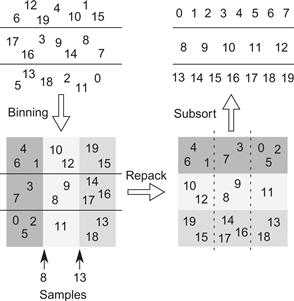
Figure 14.1 Sample sort example using a 3 × 3 matrix of buckets, where the samples for binning are 8 and 13. The keys are initially grouped into three rows of a matrix. The binning phase divides each row into buckets, one bucket for each subrange [−∞,8), [8,13), and [13,∞). The repack phase copies the buckets in a way that transposes the matrix, so that buckets for identical subranges become contiguous in memory. The subsort phase sorts each row.
In the first phase, separate rows are processed in parallel. In the second phase, separate columns are processed in parallel. There is some serial work before or after. The top-level code is shown in Listing 14.1. A production-quality C++ version would be generalized as a template with iterator arguments and a generic comparator and include extra code to ensure exception safety. These generalizations are omitted for the sake of exposition to readers who are not C++ experts.
Furthermore, our analysis will assume that the constructor T() and destructor T() are trivial enough to generate no instructions, so that the construction and destruction of array y requires only O (1) work. This is true of C-like types in C++ but generally not true if the constructor or destructor involves user-defined actions. In that case, the code shown has a Ω(N) bottleneck. Section 14.6 describes how a C++ expert can remove the bottleneck.
When the sequence is no longer than SAMPLE_SORT_CUT_OFF, the code calls Quicksort directly. The best value for SAMPLE_SORT_CUT_OFF will depend on the platform, though it should be at least big enough to subsume all cases where m = 1, since binning into a single bin is a waste of time and memory.
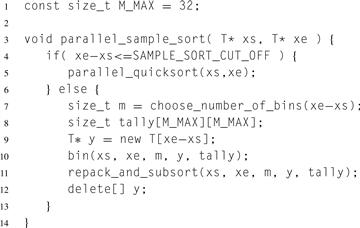
Listing 14.1 Top-level code for parallel sample sort. This code sequences the parallel phases and is independent of the parallel programming model.
14.2 Choosing the Number of Bins
If the exact number of available hardware threads (workers) is known, then using one bin per worker is best. However, in work-stealing frameworks like Cilk or TBB, the number of available workers is unknown, since the sort might be called from a nested context. Instead, a strategy of over-decomposition is used. The number of bins will be chosen so that each bin is large enough to acceptably amortize per-bin overhead. Some of the logic in function bin requires that the number of bins be a power of two. The code is shown below:
size_t choose_number_of_bins(size_t n) {
const size_t BIN_CUTOFF = 1024;
return std::min(M_MAX, size_t(1)<<floor_lg2(n/BIN_CUTOFF));
}
Function floor_lg2 is presumed to compute the function ![]() —that is, the position of the most significant 1 in the binary numeral for k.
—that is, the position of the most significant 1 in the binary numeral for k.
14.3 Binning
The binning phase involves several steps:
1. Select sample keys to demarcate the bins.
2. Organize the samples so that a key can be mapped to its bin index quickly.
3. Compute the bin index of each key.
A poor choice of demarcation samples can lead to grossly unbalanced bins. Over-sampling improves the odds against bad choices. An over-sampling factor o is chosen and om keys are selected and sorted. Then m evenly spaced samples are extracted from the sorted sequence. A good way to choose o is to make it proportional to the logarithm of the number of keys [BLM+98].
Given a linear array of sorted samples, the bin index of a key can be computed by binary search. The code for the binary search can be tightened into branchless code by rearranging the array to be an implicit binary tree. The root of the tree is stored at index 0. The children of a node with index k are stored at indices 2k + 1 and 2k + 2. Listing 14.2 shows the technique.
The code uses an implicit binary tree tree with m-1 nodes to map n keys in x to their respective bin indices. For i ∈ [0,n), the routine sets bindex[i] to the bin index of x [i]. Type bindex_type is an integral type big enough to hold an integer in the range [0,m). The routine also generates a histogram tally of bin indexes, defined as tally [b], of the number of keys with bin index b. The histogram is the sizes of the buckets in a row of our conceptual matrix.
Now the binning routine can be built. The routine divides keys in the interval [xs,xe) among m bins, and copies the keys to buckets in y.
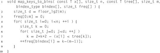
Listing 14.2 Code for mapping keys to bins.
The conceptual matrix of buckets is represented by y and tally. Each bucket of the matrix is stored in y, ordered left-to-right and top-to-bottom, with the elements within a bucket stored consecutively. Each row of tally is a running sum of bucket sizes; tally[i][j] is the sum of the sizes of buckets 0 ![]() j in row i.
j in row i.
This information suffices to reconstitute pointer bounds of a bucket. The beginning of the leftmost bucket for row i is y+i*block_size. The beginning of any other bucket is the end of the previous bucket. The end of bucket (i,j) is y+i*block_size+tally[i][j].
14.3.1 TBB Implementation
Listing 14.3 can be translated to TBB by replacing the cilk_for loop with a tbb::parallel_for and a lambda expression, so it looks like this:
tbb::parallel_for(size_t(0), m, [=,&tree](size_t i)
…
);
The lambda captures all variables by value, except for array tree, which is captured by reference, to avoid the overhead of copying an array. A subtle C++ technicality is that, although tally is captured by value, its underlying array is not copied. This is because in C and C++, a formal parameter declared as an array is treated as a pointer to its zeroth element. Hence, the lambda expression copies only the address of the array, not the array itself.
14.4 Repacking and Subsorting
The final phase of sample sort has two subphases:
1. Compute where each bin should start in the original array.
2. Move the keys from buckets into their bins, and sort them.
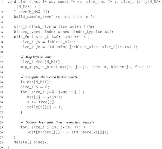
Listing 14.3 Parallel binning of keys using Cilk Plus.
The first subphase is merely a matter of summing the columns of tally. Each row of tally is a running sum of bucket sizes, so the sum of the columns yields a running sum of bin sizes. Since the value of m is typically several orders of magnitude smaller than n, the quadratic time O(m2) for computing the sums is not a major concern. It is typically too small for effective fork–join parallelism. However, it does lend itself to vector parallelism, and the array notation to do so even simplifies the source code slightly.
The second subphase does most of the work. Each parallel iteration copies a column of buckets into a bin. The bucket boundaries are found via the formulae mentioned in the discussion of method bin.
Listing 14.4 shows a Cilk Plus routine implementation of both phases.
A TBB equivalent is a matter of replacing the cilk_for statement with tbb::parallel_for, similar to the the translation in Section 14.3.1.
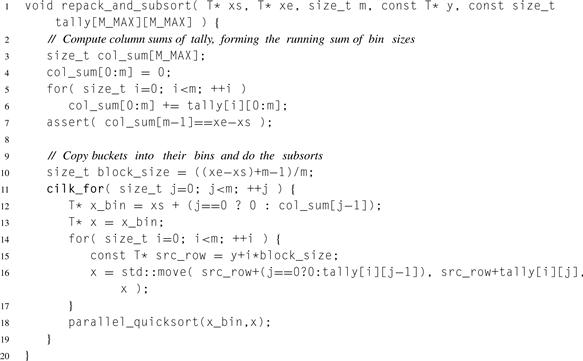
Listing 14.4 Repacking and subsorting using Cilk Plus. This is the final phase of sample sort.
14.5 Performance Analysis of Sample Sort
The asymptotic work for sample sort can be summarized as:
• Θ(mo lg mo) work to sort the input samples, over-sampled by o, where o is Θ(lg n).
• Θ(n lg m) work to bin keys into buckets.
• Θ(m2) work to compute bin sizes.
• Θ(n lg(n/m)) work to repack/subsort, assuming a subsort of k keys takes time O(k lg k).
Keeping m sufficiently small ensures that the work is dominated by the binning and repack/subsort phases, both of which scale linearly if m = Θ(p) and the log p startup time of a parallel map is insignificant.
In practice, memory bandwidth is likely to become the bottleneck. The communication between the binning and repack/subsort phases changes ownership of the bucket matrix from columns to rows. Hence, there are inherently Ω(n) memory transfers required.
There is one other potential hardware-related problem of which to be aware. If m comes close to the number of entries in the translation lookaside buffer, and each bucket is at least a page in size, then the scattering of keys among the m buckets during the binning phase may incur a severe penalty from TLB thrashing (Section 2.4.1, page 44).
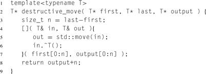
Listing 14.5 Using Cilk Plus to move and destroy a sequence, without an explicit loop!
14.6 For C++ Experts
As Section 14.1 remarked, our analysis assumes that new T[…] and delete take constant time. This is true if the constructor T() and destructor T() do nothing, as is the case for C-like types, but not always true for types with non-trivial constructors or destructors. To handle those efficiently requires rethinking the allocation/deallocation of y.
One solution is to construct the array elements in parallel and destroy them likewise. But doing so adds two more parallel phases, adding to synchronization costs and memory traffic. A faster approach is to allocate and deallocate array y as a raw memory buffer. The binning phase can copy–construct the elements into the buffer directly. The repack phase can destroy the copies as it moves them back to the original array.
A combination of array notation (Section B.8) and C++11 lambda expressions enables a concise way to write the routine that destroys the copies after moving them back to the original array, without writing any loop, as shown in Listing 14.5.
The lambda expression creates a functor that moves (Section D.3) the value of out to in, and then explicitly invokes a destructor to revert the location referenced by in to raw memory. The code is unusual in what it does with the functor. Instead of passing it to another routine, it immediately applies the functor to some arguments. The trick here is that those arguments are array sections, so the compiler has license to apply the functor in parallel.
14.7 Summary
The sample sort example showed how to do binning and packing in parallel. The key to efficient binning is over-sampling and not trying to do the binning in place as Quicksort does. The packing relied on a serial prefix scan over a histogram to calculate where items should be packed. Most of the work occurs in two parallel map operations, one for binning and one for packing. In both cases, the work is over-decomposed to provide parallel slack (Section 2.5.6).