
Chapter 6
Data Reorganization
This chapter will discuss patterns for data organization and reorganization. The performance bottleneck in many applications is just as likely, if not more likely, to be due to data movement as it is to be computation. For data-intensive applications, it is often a good idea to design the data movement first and the computation around the chosen data movements. Some common applications are in fact mostly data reorganization: searching and sorting, for instance.
In a parallel computer, additional considerations arise. First, there may be additional costs for moving data between processors and for reorganizing data for vectorization. Changes to data layout for vectorization may affect how data structures are declared and accessed. Second, scalability may depend on cache blocking and avoidance of issues such as false sharing. These issues also have data layout and possibly algorithmic implications.
Gather and scatter patterns arise from the combination of random read and write, respectively, with the map pattern. For gather, there are some special cases that can be implemented more efficiently than a completely random gather. Shifts are gathers where the data accesses are offset by fixed distances. Shifts can sometimes be implemented using vector instructions more efficiently than completely random gathers. In Chapter 7 we will also discuss the special case of the stencil pattern, which is a combination of map with a local gather over a fixed set of offsets and so can be implemented using shifts.
Gather is usually less expensive than scatter, so in general scatters should be converted to gathers when possible. This is usually only possible when the scatter addresses are known in advance for some definition of “in advance.”
Scatter raises the possibility of a collision between write locations and, with it, race conditions. We will discuss situations under which the potential for race conditions due to scatter can be avoided, as well as some deterministic versions of scatter, extending the introduction to this topic in Chapter 3.
Scatter can also be combined with local reductions which leads to a form of scatter useful for combining data that we will call merge scatter. Certain uses of scatter can also be replaced with deterministic patterns such as pack and expand. Pack and expand are also good candidates for fusion with the map pattern, since the fused versions can have significantly reduced write bandwidth. In fact, it is easiest to understand the expand pattern as an extension of a map fused with pack.
Divide-and-conquer is a common strategy for designing algorithms and is especially important in parallel algorithms, since it tends to lead to good data locality. Partitioning data, also known as geometric decomposition, is a useful strategy for parallelization. Partitioning also maps nicely onto memory hierarchies including non-uniform memory architectures. Partitioning is related to some of the optimization strategies we will discuss for stencil in Chapter 7.
Finally, we present some memory layout optimizations—in particular, the conversion of arrays of structures into structures of arrays. This conversion is an important data layout optimization for vectorization. The zip and unzip patterns are special cases of gather that can be used for such data layout reorganization.
6.1 Gather
The gather pattern, introduced in Section 3.5.4, results from the combination of a map with a random read. Essentially, gather does a number of independent random reads in parallel.
6.1.1 General Gather
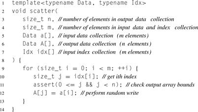
A defining serial implementation for a general gather is given in Listing 6.1. Given a collection of locations (addresses or array indices) and a source array, gather collects all the data from the source array at the given locations and places them into an output collection. The output data collection has the same number of elements as the number of indices in the index collection, but the elements of the output collection are the same type as the input data collection. If multidimensional index collections are supported, generally the output collection has the same dimensionality as the index collection, as well. A diagram showing an example of a specific gather on a 1D collection (using a 1D index) is given in Figure 6.1.
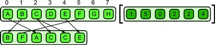
Figure 6.1 Gather pattern. A collection of data is read from an input collection given a collection of indices. This is equivalent to a map combined with a random read in the map’s elemental function.
The general gather pattern is simple but there are many special cases which can be implemented more efficiently, especially on machines with vector instructions. Important special cases include shift and zip, which are diagrammed in Figures 6.2 and 6.3. The inverse of zip, unzip, is also useful.
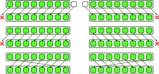
Figure 6.2 Shifts are special cases of gather. There are variants based on how boundary conditions are treated. Boundaries can be duplicated, rotated, reflected, a default value can be used, or most generally some arbitrary function can be used. Unlike a general gather, however, shifts can be efficiently implemented using vector instructions since in the interior, the data access pattern is regular.
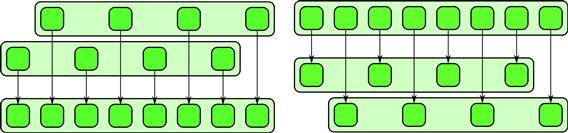
Figure 6.3 Zip and unzip (special cases of gather). These operations can be used to convert between array of structures (AoS) and structure of arrays (SoA) data layouts.
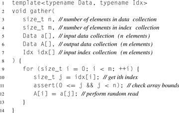
Listing 6.1 Serial implementation of gather in pseudocode. This definition also includes bounds checking (assert) during debugging as an optional but useful feature.
6.1.2 Shift
In a 1D array, the shift pattern moves data to the left or right in memory or, equivalently, to lower or higher locations, assuming we number locations from left to right. In higher dimensional arrays, shift may offset data by different amounts in each dimension. There are a few variants of shift that depend on how boundary conditions are handled, since by nature shift requires data that is “out of bounds” at the edge of the array. This missing data can be replaced with a default value, the edge value can be duplicated, or the data from the other side of the input array can be used. The last pattern is often called a rotate. It is also possible to extend the shift pattern to higher-dimensional collections to shift by larger amounts and to support additional boundary conditions, including arbitrary user-defined boundary conditions. For example, the latter can be supported by allowing arbitrary code to be executed to compute values for samples that are outside the index domain of the input collection.
Efficient implementations of shift are possible using vector operations. This is true even if complex boundary conditions are supported, since away from the boundaries, shifts still use a regular data access pattern. In this case, chunks of the input can be read into registers using vector loads, realigned using vector instructions (typically combining two separate input chunks), and then written out. More efficient implementations are typically possible if the shift amount is known at code generation time. A vectorized implementation is not strictly necessary for efficiency. Since a shift has good data locality, reading data from cache using normal read operations will still typically have good efficiency. However, vectorizing the shift can reduce the number of instructions needed.
6.1.3 Zip
The zip pattern interleaves data. A good example arises in the manipulation of complex numbers. Suppose you are given an array of real parts and an array of imaginary parts and want to combine them into a sequence of real and imaginary pairs. The zip operation can accomplish this. It can also be generalized to more elements—for example, forming triples from three input arrays. It can also be generalized to zipping and unzipping data of unlike types, as long as arrays of structures are supported in the programming model. The unzip pattern is also useful. Unzip simply reverses a zip, extracting subarrays at certain offsets and strides from an input array. For example, given a sequence of complex numbers organized as pairs, we could extract all the real parts and all the imaginary parts into separate arrays. Zip and unzip are diagrammed in Figure 6.3.
Sometimes, as in Cilk Plus, “start” and “stride” arguments are available in array sectioning operations or views, or as part of the specification of a map pattern. These can be used to implement the zip and unzip patterns, which, like shift, are often fused with the inputs and outputs of a map. Zip and unzip are also related to the computation of transposes of multidimensional arrays. Accessing a column of a row-major array involves making a sequence of memory accesses with large strides, which is just zip/unzip. The zip and unzip patterns also appear in the conversion of array of structures (AoS) to structures of arrays (SoA), data layout options that are discussed in Section 6.7.
6.2 Scatter
The scatter pattern was previously discussed in Section 3.5.5. Scatter is similar to gather, but write locations rather than read locations are provided as input. A collection of input data is then written in parallel to the write locations specified. Unfortunately, unlike gather, scatter is ill-defined when duplicates appear in the collection of locations. We will call such duplicates collisions. In the case of a collision, it is unclear what the result should be since multiple output values are specified for a single output location.
The problem is shown in Figure 6.4. Some rule is needed to resolve such collisions. There are at least four solutions: permutation scatter, which makes collisions illegal (see Figure 6.6); atomic scatter, which resolves collisions non-deterministically but atomically (see Figure 6.5); priority scatter, which resolves collisions deterministically using priorities (see Figure 6.8); and merge scatter, which resolves collisions by combining values (see Figure 6.7).
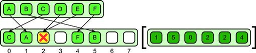
Figure 6.4 Scatter pattern. Unfortunately, the result is undefined if two writes go to the same location.
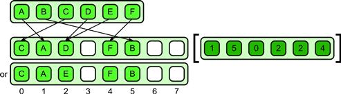
Figure 6.5 Atomic scatter pattern.
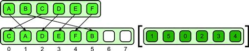
Figure 6.6 Permutation scatter pattern. Collisions are illegal.
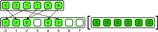
Figure 6.7 Merge scatter pattern. Associative and commutative operators are used to combine values upon collision.
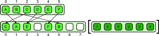
Figure 6.8 Priority scatter pattern. Every element is assigned a priority, which is used to resolve collisions.
6.2.1 Atomic Scatter
The atomic scatter pattern is non-deterministic. Upon collision, in an atomic scatter one and only one of the values written to a location will be written in its entirety. All other values written to the same location will be discarded. See Figure 6.5 for an example. Note that we do not provide a rule saying which of the input items will be retained. Typically, it is the last one written but in parallel implementations of atomic scatter the timing of writes is non-deterministic.
This pattern resolves collisions atomically but non-deterministically. Use of this pattern may result in non-deterministic programs. However, it is still useful and deterministic in the special case that all input data elements written to the same location have the same value. A common example of this is the writing of true Boolean flags into an output array that has initially been cleared to false. In this case, there is an implicit OR merge between the written values, since only one of the writes needs to update the output location to turn it into a true, and the result is the same whichever write succeeds.
Examples of the use of atomic scatter include marking pairs in collision detection, and computing set intersection or union as are used in text databases. Note that these are both examples where Boolean values may be used.
6.2.2 Permutation Scatter
The permutation scatter pattern simply states that collisions are illegal; in other words, legal inputs should not have duplicates. See Figure 6.6 for an example of a legal permutation scatter. Permutation scatters can always be turned into gathers, so if the addresses are known in advance, this optimization should be done. Checking for collisions, to report them as errors, can be expensive but can be done in a debugging-only mode if necessary.
The danger with permutation scatter is that programmers will use it when addresses do in fact have collisions. The resulting program may work but would depend upon undefined behavior exhibited by a particular implementation. Later on, when the implementation changes, this behavior may change and the program will be “broken.” That is why it is better for implementations to actually check for collisions and report them, at least in debug mode.
Of course this problem is true for any program that depends on any undefined behavior. The issues with undefined behavior here are similar to the safety issues that arise with out-of-bounds array accesses in some programming languages. A program with an out-of-bounds access may work fine on some implementations but produce incorrect results on other implementations or simply crash. Therefore, some languages introduce array-bounds checking, but this can be expensive.
Examples of use of the permutation scatter include FFT scrambling, matrix/image transpose, and unpacking. Note that the first two of these could be (and usually should be) implemented with an equivalent gather.
6.2.3 Merge Scatter
In the merge scatter pattern, associative and commutative operators are provided to merge elements in case of a collision. Both properties are required, normally, since scatters to a particular location could occur in any order. In Figure 6.7, an example is shown that uses addition as the merge operator.
One problem with this pattern is that it, as with the reduction pattern, depends on the programmer to define an operator with specific algebraic properties. However, the pattern could be extended to support non-deterministic, but atomic, read–modify–write when used with non-associative operators. Such an extension would be a simple form of the transaction pattern.
Merge scatter can be used to implement histograms in a straightforward way by using the addition operation. Merge scatter can also be used for the computation of mutual information and entropy, as well as for database updates. The examples given earlier for atomic scatter of Boolean values could be interpreted as merge scatters with the OR operation.
6.2.4 Priority Scatter
In the priority scatter pattern, an example of which is given in Figure 6.8, every element in the input array for a scatter is assigned a priority based on its position. This priority is used to decide which element is written in case of a collision. By making the priorities higher for elements that would have been written later in a serial ordering of the scatter, the scatter is made not only deterministic but also consistent with serial semantics.
Consider the serial defining implementation of scatter in Listing 6.2. If there is a collision (two addresses writing the to same location) in the serial implementation of scatter, this is not normally considered a problem. Later writes will overwrite previous writes, giving a deterministic result.
Priorities for the priority scatter can be chosen to mimic this behavior, also discussed in Listing 6.2, making it easier to convert serial scatters into parallel scatters.
Another interesting possibility is to combine merge and priority scatter so that writes to a given location are guaranteed to be ordered.
Listing 6.2 Serial implementation of scatter in pseudocode. Array bounds checking is included in this implementation for clarity but is optional.
This combined priority merge pattern is, in fact, fundamental to a massively parallel system available on nearly every personal computer: 3D graphics rendering. The pixel “fragments” written to the framebuffer are guaranteed to be in the same order that the primitives are submitted to the graphics system and several operations are available for combining fragments into final pixel values.
6.3 Converting Scatter to Gather
Scatter is more expensive than gather for a number of reasons. For memory reads, the data only has to be read into cache. For memory writes, due to cache line blocking, often a whole cache line has to be read first, then the element to be modified is updated, and then the whole cache line is written back. So a single write in your program may in fact result in both reads and writes to the memory system.
In addition, if different cores access the same cache line, then implicit communication and synchronization between cores may be required for cache coherency. This needs to be done by the hardware even if there are no actual collisions if writes from different cores go to the same cache line. This can result in significant extra communication and reduced performance and is generally known as false sharing.
These problems can be avoided if the addresses are available “in advance.” All forms of scatter discussed in Section 6.2 can be converted to gathers if the addresses are known in advance. It is also possible to convert the non-deterministic forms of scatter into deterministic ones by allocating cores to each output location and by making sure the reads and processing for each output location are done in a fixed serial order.
However, a significant amount of processing is needed to convert the addresses for a scatter into those for a gather. One way to do it is to actually perform the scatter, but scatter the source addresses rather than the data. This builds a table that can then be used for the gather. The values in such a table will be deterministic if the original scatter was deterministic. Atomic scatters can be converted to priority scatters in this step, which will affect only the process of building the table, not the performance of the gather.
Since extra processing is involved, this approach is most useful if the same pattern of scatter addresses will be used repeatedly so the cost can be amortized. Sometimes library functions include an initialization or “planning” process in which the configuration and size of the input data are given. This is a good place to include such computation.
6.4 Pack
The pack pattern is used to eliminate unused elements from a collection. The retained elements are moved so that they are contiguous in memory which can improve the performance of later memory accesses and vectorization. Many common uses of the scatter pattern can be converted to packs. One advantage of a pack over a scatter is that a pack is deterministic by nature, unlike the case with scatter.
Pack can be implemented by combining scan and a conditional scatter. First, convert the input array of Booleans into integer 0’s and 1’s, and then perform an exclusive scan of this array with an initial value of 1 and the addition operation. This produces a set of offsets into an output array where each data input to be kept should be written. This can be done with a permutation scatter since locations will not be duplicated. Note, however, that the scatter should be conditional, since only the locations with a true flag should result in a write. An example of the pack operation is diagrammed in Figure 6.9.

Figure 6.9 Pack pattern.
The inverse of the pack operation is unpack, which, given the same data on which elements were kept and which were discarded, can place elements back in their original locations. Since the discarded values are unknown, a default value can be used for these locations. An example of the unpack pattern is diagrammed in Figure 6.10.
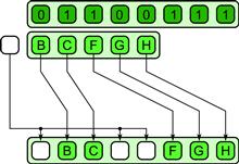
Figure 6.10 Unpack pattern.
A generalization of the pack pattern is the split pattern. This pattern is shown in Figure 6.11. Rather than discarding elements as with pack, in the split operation elements are moved to either the upper or lower half of an output collection based on the value of some per-element predicate. Of course, split can be emulated with two packs using complementary conditions, but split can usually be implemented more efficiently than two separate packs. Split also does not lose information like pack does. The inverse of split, unsplit, is shown in Figure 6.12. There is some relationship between these patterns and zip and unzip discussed in Section 6.1.3, but unpack are specific patterns that can usually be implemented more efficiently than the more general split and unsplit patterns.
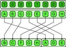
Figure 6.11 Split pattern.
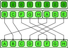
Figure 6.12 Unsplit pattern.
Interestingly, control flow can be emulated on a SIMD machine given pack and unpack operations or, better yet, split and unsplit operations [LLM08, HLJH09]. Unlike the case with masking, such control flow actually avoids work and does not suffer from a reduction in coherency for divergent control flow. However, without hardware support it does have higher overhead, so most implementations emulating control flow on SIMD machines use the masking approach.
Split can be generalized further by using multiple categories. The Boolean predicate can be considered as a classification of input elements into one of two categories. It is also reasonable to generalize split to support more than two categories. Support for multiple categories leads to the bin pattern, shown in Figure 6.13 for four categories. The bin pattern appears in such algorithms as radix sort and pattern classification and can also be used to implement category reduction.
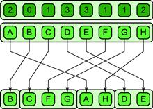
Figure 6.13 The bin pattern generalizes the split pattern to multiple categories.
Note in the case of both the split and bin patterns that we would like to have, as a secondary output from these operations, the number of elements in each category, some of which may be empty. This is also useful for the pack pattern. In the case of pack this is the size of the output collection. Note that the output of the pack pattern might be empty!
Normally we want both split and bin to be stable, so that they preserve the relative order of their inputs. This allows these operations to be used to implement radix sort, among other applications.
One final generalization of pack, the expand pattern, is best understood in the context of a pack fused with a map operation (see Figure 6.15). When pack is fused with map, each element can output zero or one element. This can be generalized so that each element can output any number of elements, and the results are fused together in order.
6.5 Fusing Map and Pack
Pack can be fused to the output of a map as shown in Figure 6.14. This is advantageous if most of the elements of the map are discarded.
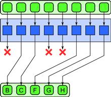
Figure 6.14 Fusion of map and pack patterns.
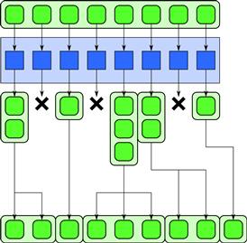
Figure 6.15 Expand pattern. This permits the implementation of applications that result in data amplification. It also provides a form of dynamic memory allocation.
For example, consider the use of this pattern in a collision detection problem. In such a problem, we have a large number of objects and want to detect which pairs overlap in space. We will call each overlapping pair a collision, and the output of the algorithm is a list of all the collisions. We might have a large number of potentially colliding pairs of objects, but only a few that actually collide. Fusing a map to check pairs for collision, with a pack to store only actual collisions, will reduce the total amount of output bandwidth to be proportional to the results reported and not the number of pairs tested.
The expand pattern is best understood in the context of a pack fused with a map operation. Compare Figure 6.14 with Figure 6.15. When pack is fused with map, each element can output zero or one element. This is generalized in the expand pattern so that each element can output any number of elements, and the results are output in order.
For example, suppose you wanted to create a parallel implementation of L-system substitution. In L-system substitution, the input and output are strings of characters. Every element of the input string might get expanded into a new string of characters, or deleted, according to a set of rules. Such a pattern is often used in computer graphics modeling where the general approach is often called data amplification. In fact, this pattern is supported in current graphics rendering pipelines in the form of geometry shaders. To simplify implementation, the number of outputs might be bounded to allow for static memory allocation, and this is, in fact, done in geometry shaders. This pattern can also be used to implement variable-rate output from a map, for example, as required for lossless compression.
As with pack, fusing expand with map makes sense since unnecessary write bandwidth can then be avoided. The expand pattern also corresponds to the use of push_back on C++ STL collections in serial loops.
The implementation of expand is more complex than pack but can follow similar principles. If the scan approach is used, we scan integers representing the number of outputs from each element rather than only zeros and ones. In addition, we should tile the implementation so that, on a single processor, a serial “local expand” is used which is trivial to implement.
6.6 Geometric Decomposition and Partition
A common strategy to parallelize an algorithm is to divide up the computational domain into sections, work on the sections individually, and then combine the results. Most generally, this strategy is known as divide-and-conquer and is also used in the design of recursive serial algorithms. The parallelization of the general form of divide-and-conquer is supported by the fork–join pattern, which is discussed extensively in Chapter 8.
Frequently, the data for a problem can also be subdivided following a divide-and-conquer strategy. This is obvious when the problem itself has a spatially regular organization, such as an image or a regular grid, but it can also apply to more abstract problems such as sorting and graphs. When the subdivision is spatially motivated, it is often also known as geometric decomposition.
As a special case of geometric decomposition, the data is subdivided into uniform non-overlapping sections that cover the domain of computation. We will call this the partition pattern. An example of a partition in 1D is shown in Figure 6.16. The partition pattern can also be applied in higher dimensions as is shown in Figure 6.17.
![]()
Figure 6.16 Partitioning. Data is divided into non-overlapping, equal-sized regions.
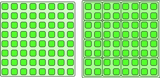
Figure 6.17 Partitioning in 2D. The partition pattern can be extended to multiple dimensions.
The sections of a partition are non-overlapping. This is an important property to avoid write conflicts and race conditions. A partition is often followed by a map over the set of sections with each instance of the elemental function in the map being given access to one of the sections. In this case, if we ensure that the instance has exclusive access to that section, then within the partition serial scatter patterns, such as random writes, can be used without problems with race conditions. It is also possible to apply the pattern recursively, subdividing a section into subsections for nested parallelism. This can be a good way to map a problem onto hierarchically organized parallel hardware.
These diagrams show only the simplest case, where the sections of the partition fit exactly into the domain. In practice, there may be boundary conditions where partial sections are required along the edges. These may need to be treated with special-purpose code, but even in this case the majority of the sections will be regular, which lends itself to vectorization. Ideally, to get good memory behavior and to allow efficient vectorization, we also normally want to partition data, especially for writes, so that it aligns with cache line and vectorization boundaries. You should be aware of how data is actually laid out in memory when partitioning data. For example, in a multidimensional partitioning, typically only one dimension of an array is contiguous in memory, so only this one benefits directly from spatial locality. This is also the only dimension that benefits from alignment with cache lines and vectorization unless the data will be transposed as part of the computation. Partitioning is related to strip-mining the stencil pattern, which is discussed in Section 7.3.
Partitioning can be generalized to another pattern that we will call segmentation. Segmentation still requires non-overlapping sections, but now the sections can vary in size. This is shown in Figure 6.18. Various algorithms have been designed to operate on segmented data, including segmented versions of scan and reduce that can operate on each segment of the array but in a perfectly load-balanced fashion, regardless of the irregularities in the lengths of the segments [BHC+93]. These segmented algorithms can actually be implemented in terms of the normal scan and reduce algorithms by using a suitable combiner function and some auxiliary data. Other algorithms, such as quicksort [Ble90, Ble96], can in turn be implemented in a vectorized fashion with a segmented data structure using these primitives.
![]()
Figure 6.18 Segmentation. If data is divided into non-uniform non-overlapping regions, it can be referred to as segmentation (a generalization of partitioning).
In order to represent a segmented collection, additional data is required to keep track of the boundaries between sections. The two most common representations are shown in Figure 6.19. Using an array of Boolean flags to mark the start point of each segment is convenient and is useful for efficient implementation of segmented scans and reductions. The Boolean flags can be stored reasonably efficiently using a packed representation. However, this representation does not allow zero-length segments which are important for some algorithms. Also, it may be space inefficient if segments are very long on average. An alternative approach is to record the start position of every segment. This approach makes it possible to represent empty segments. Note that differences of adjacent values also give the length of each segment. The overall length of the collection can be included as an extra element in the length array to make this regular and avoid a special case.
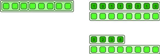
Figure 6.19 Segmentation representations. Various representations of segmented data are possible. The start of each segment can be marked using an array of flags. Alternatively, the start point of each segment can be indicated using an array of integers. The second approach allows zero-length segments; the first does not.
Many of the patterns we have discussed could output segmented collections. For example, the output of the expand, split, and bin patterns, discussed in Section 6.4, could be represented as a segmented collection. Of course it is always possible to discard the segment start data and so “flatten” a segmented collection. It would also be possible to support nested segmentation, but this can always be represented, for any given maximum nesting depth, using a set of segment-start auxiliary arrays [BHC+93, Ble90]. It is possible to map recursive algorithms, such as quicksort, onto such data representations [Ble96, Ble90].
Various extensions to multidimensional segmentations are possible. For example, you could segment along each dimension. A kD-tree-like generalization is also possible, where a nested segmentation rotates among dimensions. However, the 1D case is probably the most useful.
6.7 Array of Structures vs. Structures of Arrays
For vectorization, data layout in memory may have to be modified for optimal performance.
The usual approach to data abstraction is to declare structures representing some object and then create collections of that structure. For example, suppose we want to simulate a collection of particles. Every particle will have a state with a collection of values, such as velocity, mass, color, etc. You would normally declare a structure containing all the state variables needed for one particle. A particle simulation evolves the state of a set of particles over time by applying a function to each particle’s state, generating a new state. For such a simulation, you would need a collection holding the state of the set of particles, which is most obviously represented by defining an array of structures. Code for this data organization is shown in Listing 6.3. Conceptually, the data is organized as shown on the left side of Figure 6.20.
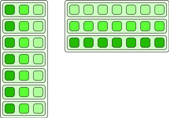
Figure 6.20 Array of structures (AoS) versus structure of arrays (SoA). SoA form is typically better for vectorization and avoidance of false sharing. However, if the data is accessed randomly, AOS may lead to better cache utilization.
However, the array of structures form has the problem that it does not align data well for vectorization or caching, especially if the elements of the structure are of different types or the overall length of the structure does not lend itself to alignment to cache line boundaries.
In this case, an alternative approach is to use one collection for each element of state in the structure, as on the right side of Figure 6.20. This is known as the structure of arrays, or SoA, layout. Now if we apply the map pattern to this, vectorization of an elemental function is much easier, and we can also cleanly break up the data to align to cache boundaries. It is also easier to deal with data elements that vary in size.
Unfortunately, in languages like C and Fortran, changing the data layout from SoA to AoS results in significant changes to data structures and also tends to break data encapsulation. Listing 6.4 shows the reorganization required to convert the data structures declared in Listing 6.3 to SoA form.
Figure 6.21 shows how these two options lay out data in memory and how padding can be added to help with cache alignment in both cases. For SoA form, we can add padding to each structure to maintain cache alignment and avoid false sharing but this can add a significant amount of overhead to each structure. If we do not add this padding, misalignments may significantly increase computation time and will also complicate vectorization. In AoS form, padding is not really needed, but even if we do include it, it tends to be only required at the boundaries. If the collections are large, then AoS form has large internal regions of coherently organized data that can be efficiently vectorized even without internal padding.
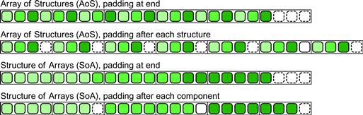
Figure 6.21 Data layout options for arrays of structures and structures of arrays. Data can be laid out structure-by-structure, structure-by-structure with padding per structure, or, for structure of array, array-by-array or array-by-array with padding. The structure of array form, either with or without padding, makes vectorization much easier.
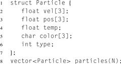
Listing 6.3 Array of structures (AoS) data organization.
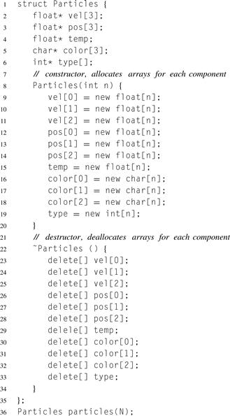
Listing 6.4 Structure of arrays (SoA) data organization.
Unfortunately, the SoA form is not ideal in all circumstances. For random or incoherent circumstances, gathers are used to access the data and the SoA form can result in extra unneeded data being read into cache, thus reducing performance. In this case, use of the AoS form instead will result in a smaller working set and improved performance. Generally, though, if the computation is to be vectorized, the SoA form is preferred.
6.8 Summary
We have presented some data reorganization patterns and discussed some important issues around data layout.
Data reorganization patterns include scatter and gather, both of which have several special cases. Gather is a pattern that supports a set of parallel reads, while scatter supports a set of parallel writes. Shift and zip, as well as their inverses, unshift and unzip, are special cases of gather that can be more efficiently vectorized. Scatter has a potential problem when multiple writes to the same location are attempted. This problem can be resolved in several ways. Atomic scatters ensure that upon such collisions correct data is written, but the order is still non-deterministic. Permutation scatters simply declare collisions to be illegal and the result undefined, but it can be expensive to check for collisions, so this is usually only supportable in a debug mode. Priority scatters order the writes by priority to mimic the behavior of a random write in a loop, while merge scatters use an associative and commutative operation to combine the values involved in a collision. All forms of scatter are more expensive than gather, so scatters should normally be converted to gathers whenever possible. This is always possible if the scatter locations are known in advance.
The pack pattern can replace many uses of scatter but has the advantage that it is deterministic. The pack pattern has several generalizations, including the split, bin, and expand patterns.
A poor data layout can negatively impact performance and scalability, so it should be considered carefully. Unfortunately, some of the optimizations considered in this chapter are not always applicable. In particular, the effectiveness of the structure of arrays (SoA) form depends on how many operations over the data can be vectorized versus how often the data is accessed randomly. Cache effects such as false sharing can also dramatically affect performance, and many other computer architecture issues come to play in practice. See Appendix A for suggestions of additional reading on this topic.