
Chapter 9
Pipeline
Online algorithms are important for modern computing. In an online algorithm, processing starts before all the input is available, and the output starts to be written before all processing is complete. In other words, computing and I/O take place concurrently. Often the input is coming from real-time sources such as keyboards, pointing devices, and sensors. Even when all the input is available, it is often on a file system, and overlapping the algorithm with input/output can yield significant improvements in performance. A pipeline is one way to achieve this overlap, not only for I/O but also for computations that are mostly parallel but require small sections of code that must be serial.
This chapter covers a simple pipeline model embodied in the TBB parallel_pipeline template. It shows the mechanics of using that template, as well as how to imitate it in Cilk Plus in limited circumstances. This chapter also touches on the general issue of mandatory parallelism versus optional parallelism, which becomes important when pipelines are generalized beyond the simple model. In particular, care must be taken to avoid producer/consumer deadlock when using optional parallelism to implement a pipeline.
9.1 Basic Pipeline
A pipeline is a linear sequence of stages. Data flows flows through the pipeline, from the first stage to the last stage. Each stage performs a transform on the data. The data is partitioned into pieces that we call items. A stage’s transformation of items may be one-to-one or may be more complicated. A serial stage processes one item at a time, though different stages can run in parallel.
Pipelines are appealing for several reasons:
• Early items can flow all the way through the pipeline before later items are even available. This property makes pipelines useful for soft real-time and online applications. In contrast, the map pattern (Chapter 4) has stronger synchronization requirements: All input data must be ready at the start, and no output data is ready until the map operation completes.
• Pipeline composition is straightforward. The output of a pipeline can be fed into the input of a subsequent pipeline.
• A serial pipeline stage maps naturally to a serial I/O device. Even random-access devices such as disks behave faster when access to them is serial. By having separate stages for computation and I/O, a pipeline can be an effective means of overlapping computation and I/O.
• Pipelines deal naturally with resource limits. The number of items in flight can be throttled to match those limits. For example, it is possible for a pipeline to process large amounts of data using a fixed amount of memory.
• The linear structure makes it it easy to reason about deadlock freedom, unlike topologies involving cycles or merges.
• With some discipline, each stage can be analyzed and debugged separately.
A pipeline with only serial stages has a fundamental speedup limit similar to Amdahl’s law, but expressed in terms of throughput. The throughput of the pipeline is limited to the throughput of the slowest serial stage, because every item must pass through that stage one at a time. In asymptotic terms, ![]() , so pipelines provide no asymptotic speedup ! Nonetheless, the hidden constant factor can make such a pipeline worth the effort. For example, a pipeline with four perfectly balanced stages can achieve a speedup of four. However, this speedup will not grow further with more processors: It is limited by the number of serial stages, as well as the balance between them.
, so pipelines provide no asymptotic speedup ! Nonetheless, the hidden constant factor can make such a pipeline worth the effort. For example, a pipeline with four perfectly balanced stages can achieve a speedup of four. However, this speedup will not grow further with more processors: It is limited by the number of serial stages, as well as the balance between them.
9.2 Pipeline with Parallel Stages
Introducing parallel stages can make a pipeline more scalable. A parallel stage processes more than one item at a time. Typically it can do so because it has no mutable state. A parallel stage is different from a serial stage with internal parallelism, because the parallel stage can process multiple input items at once and can deliver the output items out of order.
The introduction of parallel stages introduces a complication to serial stages. In a pipeline with only serial stages, each stage receives items in the same order. But when a parallel stage intervenes between two serial stages, the later serial stage can receive items in a different order from the earlier stage. Some applications require consistency in the order of items flowing through the serial stages, and usually the requirement is that the final output order be consistent with the initial input order. The data compression example in Chapter 12 is a good example of this requirement.
Intel TBB deals with the ordering issue by defining three kinds of stages:
• parallel: Processes incoming items in parallel
• serial_out_of_order: Processes items one at a time, in arbitrary order
• serial_in_order: Processes items one at a time, in the same order as the other serial_in_order stages in the pipeline
The difference in the two kinds of serial stages has no impact on asymptotic speedup. The throughput of the pipeline is still limited by the throughput of the slowest stage. The advantage of the serial_out_of_order kind of stage is that by relaxing the order of items, it can improve locality and reduce latency in some scenarios by allowing an item to flow through that would otherwise have to wait for its predecessor.
The simplest common sequence of stages for parallel_pipeline is serial–parallel–serial, where the serial stages are in order. There are two ways to picture such a pipeline. The first is to draw each stage as a vertex in a graph and draw edges indicating the flow of data. Figure 9.1 pictures a serial–parallel–serial pipeline this way.
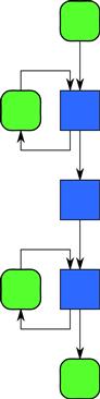
Figure 9.1 Serial–parallel–serial pipeline. The two serial stages have feedback loops that represent updating their state. The middle stage is stateless; thus multiple invocations of it can run in parallel.
The parallel stage is distinguished by not having a feedback loop like the two serial stages do. This way of drawing a pipeline is concise and intuitive, though it departs from the diagrams in other sections because a single vertex handles a sequence of data items and not a single piece of data.
An alternative is to show one vertex per stage invocation, as in Figure 9.2. The parallel stage is distinguished by not having any horizontal dependencies in the picture. It gives an intuitive analysis of the work and span. For example, assume each serial task in the picture takes unit time, and each parallel task takes four units of time. For n input items, the work T1 is 6n since each item requires two serial tasks and one parallel task. The span T∞ is n + 5, because the longest paths through the graph pass through some combination of n + 1 serial tasks before and after passing through one parallel task. Speedup is thus limited to ![]() , which approaches 6 as n approaches ∞. This sort of picture is not possible if the pipeline computation has serial_out_of_order stages, which are beyond the DAG model of computation (Section 2.5.6).
, which approaches 6 as n approaches ∞. This sort of picture is not possible if the pipeline computation has serial_out_of_order stages, which are beyond the DAG model of computation (Section 2.5.6).
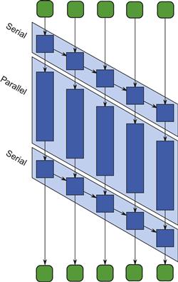
Figure 9.2 DAG model of pipeline in Figure 9.1. This picture shows the DAG model of computation (Section 2.5.6) for the pipeline in Figure 9.1, assuming there are five input items. To emphasize the opportunity for parallelism, each box for a parallel task is scaled to show it taking four times as much time as a serial task.
9.3 Implementation of a Pipeline
There are two basic approaches to implementing a pipeline:
• A worker is bound to a stage and processes items as they arrive. If the stage is parallel, it may have multiple workers bound to it.
• A worker is bound to an item and carries the item through the pipeline [MSS04]. When a worker finishes the last stage, it goes to the first stage to pick up another item.
The difference can be viewed as whether items flow past stages or stages flow past items. In Figure 9.2, the difference is whether a worker deals with tasks in a (slanted) row or tasks in a column.
The two approaches have different locality behavior. The bound-to-stage approach has good locality for internal state of a stage, but poor locality for the item. Hence, it is better if the internal state is large and item state is small. The bound-to-item approach is the other way around.
The current implementation of TBB’s parallel_pipeline uses a modified bind-to-item approach. A worker picks up an available item and carries it through as many stages as possible. If a stage is not ready to accept another item, the worker parks the item where another worker can pick it up when the stage is ready to accept it. After a worker finishes applying a serial stage to an item, it checks if there is a parked input item waiting at that state, and if so spawns a task that unparks that item and continues carrying it through the pipeline. In this way, execution of a serial stage is serialized without a mutex.
The parking trick enables greedy scheduling —no worker waits to run a stage while there is other work ready to do. But it has the drawback of eliminating any implicit space bounds. Without the parking trick, a pipeline with P workers uses at most about P more space than serial execution, since the space is no worse than P copies of the serial program running. But the parking trick is equivalent to creating suspended copies of the serial program, in addition to the P running copies. TBB addresses the issue by having the user specify an upper bound on the number of items in flight.
9.4 Programming Model Support for Pipelines
Understanding the various syntaxes for pipelines is not only good for using them but also reveals some design issues. Our running example is a series–parallel–series pipeline. The three stages run functors f, g, and h, in that order. Listing 9.1 shows the serial code. Functions f and h are assumed to require serial in-order stages, and g is assumed to be okay to run as a parallel stage.
9.4.1 Pipeline in TBB
The TBB parallel_pipeline template requires that a stage map one input item to one output item. The overall steps for building a pipeline in TBB are:
• Construct a filter_t<X,Y> for each stage. Type X is the input type; type Y is the output type. The first stage must have type filter_t<void,…>. The last stage must have type filter_t<…,void>.
• Glue the stages together with operator&. The output type of a stage must match the input type of the next stage. The type of a filter_t<X,Y> glued to a filter_t<Y,Z> is a filter_t<X,Z>. From a type system perspective, the result acts just like a a big stage. The top-level glued result must be a filter_t<void,void>.
• Invoke parallel_pipeline on the filter_t<void,void>. The call must also provide an upper bound on the number of items in flight.
Listing 9.2 shows a TBB implementation of our running example. It illustrates the details of constructing stages. Function make_filter builds a filter_t object. Its arguments specify the kind of stage and the mapping of items to items. For example, the middle stage is a parallel stage that uses functor g to map input items of type T to output items of type U.
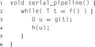
Listing 9.1 Serial implementation of a pipeline, with stages f, g, and h.
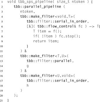
Listing 9.2 Pipeline in TBB. It is equivalent to the serial pipeline in Listing 9.1, except that the stages run in parallel and the middle stage processes multiple items in parallel.
The first and last stages use side effects to communicate with the rest of the program, and the corresponding input/output types are void. The last stage is declared as mapping items from U to void and uses side effects to output items. Conversely, the first stage is declared as mapping items from void to T and uses side effects to input items.
The first stage is also special because each time it is invoked it has to return an item or indicate that there are no more items. The TBB convention is that it takes an argument of type flow_control&. If it has no more items to output, it calls method stop on that argument, which indicates that there are no more items, and the currently returned item should be ignored.
9.4.2 Pipeline in Cilk Plus
Pipelines with an arbitrary number of stages are not expressible in Cilk Plus. However, clever use of a reducer enables expressing the common case of a serial–parallel–serial pipeline. The general approach is:
1. Invoke the first stage inside a serial loop.
2. Spawn the second stage for each item produced by the first stage and feed its output to a consumer reducer.
3. Invoke the third stage from inside the consumer reducer, which enforces the requisite serialization.
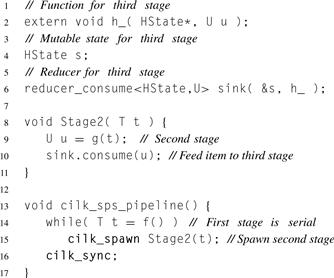
Listing 9.3 Pipeline in Cilk Plus equivalent to the serial pipeline in Listing 9.1. This version uses function h_ instead of functor h for reasons explained in the text.
Though the template for the consumer reducer could be written for our functor h, doing so complicates writing the template. So, to simplify exposition, we assume that the third stage is defined by a function h_ that takes two arguments: a pointer to its mutable state and the value of an input item. These assumptions work nicely for the bzip2 example (Section 12.4).
Listing 9.3 shows the mechanics of writing the pipeline. The intra-stage logic is close to that in Listing 9.2. All that differs is how the stages communicate. Whereas in the TBB code stages communicate through arguments and return values, here the communication is ad hoc. The second stage of the TBB version returned its result value u to send it on to the third stage. Its Cilk Plus equivalent sends u to the third stage by invoking sink.consume(u). Unlike the TBB version, the first stage does not really need any wrapper at all. It is just a serial loop that gets items and spawns the second stage.
Now reducer_consume can be explained. Recall how Section 8.10 described reducers in terms of algebraic monoids. The reducer here is manipulating side effects, namely updates to HState. At first glance, this imperative nature seems contrary to a algebraic monoid, but there is a monoid lurking behind reducer_consumer: list concatenation, or what mathematicians call the free monoid. Suppose all processing by the third stage function h_ could be deferred until after the cilk_sync. Then each view could be a list of U. Two views could be joined by concatenating their lists, and since concatenation is associative, the final list of U would be independent of whether execution really forked or not.
The implementation described so far is mathematically clean but has two drawbacks:
• It loses potential parallelism by not overlapping invocations of h_ with invocations of the other stages.
Indeed, the latter objection is severe for the bzip2 example, because each item is a pointer to a compressed block of data waiting to be written to disk. Retaining all those blocks in memory would limit how big a file bzip2 can process. However, observe that the list in the leftmost view can be fed to h_ immediately. There is no reason to build a list for the leftmost view. Only lists in other views need to be deferred.
So reducer_consumer joins views using the following rules:
Listing 9.4 shows the implementation. The list is non-empty only if actual parallelism occurs, since only then is there is a non-leftmost view. Section 11.2.1 explains the general mechanics of creating a View and Monoid for a cilk::reducer.
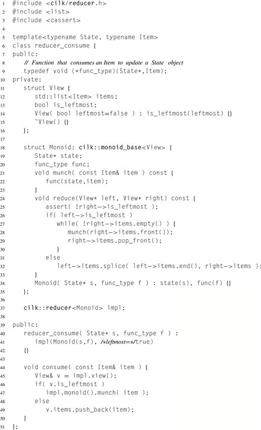
Listing 9.4 Defining a reducer for serializing consumption of items in Cilk Plus.
From a mathematical perspective, the fields of View are monoid values:
• View::items is a value in a list concatenation monoid.
• View::is_leftmost is a value in a monoid over boolean values, with operation ![]() .
.
Both of these operations are associative but not commutative.
9.5 More General Topologies
Pipelines can be generalized to non-linear topologies, and stages with more complex rules. TBB 4.0 has such a framework, in namespace tbb::flow. This framework also lifts the restriction that each stage map exactly one input item to one output item. With more complex topologies comes power, but more programmer responsibility.
The additional power of the TBB 4.0 tbb::flow framework comes with additional responsibility. The framework lifts most of the restrictions of parallel_pipeline while still using a modified bound-to-item approach that avoids explicit waiting. It allows stages to perform one-to-many and many-to-one mappings, and topologies can be non-linear and contain cycles. Consequently, designing pipelines in that framework requires more attention to potential deadlock if cycles or bounded buffers are involved.
9.6 Mandatory versus Optional Parallelism
Different potential implementations of a pipeline illustrate the difference between optional parallelism and mandatory parallelism. Consider a two-stage pipeline where the producer puts items into a bounded buffer and the consumer takes them out of the buffer. There is no problem if the producer and consumer run in parallel. But serial execution is tricky. If a serial implementation tries to run the producer to completion before executing the consumer, the buffer can become full and block further progress of the producer. Alternatively, trying to run the consumer to completion before executing the producer will hang. The parallelism of the producer and consumer is mandatory: The producer and consumer must interleave to guarantee forward progress. Programs with mandatory parallelism can be much harder to debug than serial programs.
The TBB parallel_pipeline construct dodges the issue by restricting the kinds of pipelines that can be built. There is no explicit waiting—a stage is invoked only when its input item is ready, and must emit exactly one output item per invocation. Thus, serial operation of parallel_pipeline works by carrying one item at a time through the entire pipeline. No buffering is required. Parallel operation does require buffering where a parallel stage feeds into a serial stage and the serial stage is busy. Because parallel_pipeline requires the user to specify its maximum number n of items in flight level, the buffer can be safely bounded to n.
9.7 Summary
The pipeline pattern enables parallel processing of data to commence without having all of the data available, and it also allows data to be output before all processing is complete. Thus, it is a good fit for soft real-time situations when data should be processed as soon as it becomes available. It also allows overlap of computation with I/O and permits computations on data that may not fit in memory in its entirety. The weakness of pipelines is scalability—the throughput of a pipeline is limited to the throughput of its slowest serial stage. This can be addressed by using parallel pipeline stages instead of serial stages to do work where possible. The TBB implementation uses a technique that enables greedy scheduling, but the greed must be constrained in order to bound memory consumption. The user specifies the constraint as a maximum number of items allowed to flow simultaneously through the pipeline. Simple pipelines can be implemented in Cilk Plus by creative use of reducers.