
Chapter 2
Background
Good parallel programming requires attention to both the theory and the reality of parallel computers. This chapter covers background material applicable to most forms of parallel programming, including a (short) review of relevant computer architecture and performance analysis topics. Section 2.1 introduces basic vocabulary and the graphical notation used in this book for patterns and algorithms. Section 2.2 defines and names some general strategies for designing parallel algorithms. Section 2.3 describes some general mechanisms used in modern processors for executing parallel computations. Section 2.4 discusses basic machine architecture with a focus on mechanisms for parallel computation and communication. The impact of these on parallel software design is emphasized. Section 2.5 explains performance issues from a theoretical perspective, in order to provide guidance on the design of parallel algorithms. Section 2.6 discusses some common pitfalls of parallel programming and how to avoid them. By the end of this chapter, you should have obtained a basic understanding of how modern processors execute parallel programs and understand some rules of thumb for scaling performance of parallel applications.
2.1 Vocabulary and Notation
The two fundamental components of algorithms are tasks and data. A task operates on data, either modifying it in place or creating new data. In a parallel computation multiple tasks need to be managed and coordinated. In particular, dependencies between tasks need to be respected. Dependencies result in a requirement that particular pairs of tasks be ordered. Dependencies are often but not always associated with the transfer of data between tasks. In particular, a data dependency results when one task cannot execute before some data it requires is generated by another task. Another kind of dependency, usually called a control dependency, results when certain events or side effects, such as those due to I/O operations, need to be ordered. We will not distinguish between these two kinds of dependency, since in either case the fundamental requirement is that tasks be ordered in time.
For task management the fork–join pattern is often used in this book. In the fork–join pattern, new serial control flows are created by splitting an existing serial control flow at a fork point. Conversely, two separate serial control flows are synchronized by merging them together at a join point. Within a single serial control flow, tasks are ordered according to the usual serial semantics. Due to the implicit serial control flow before and after these points, control dependencies are also needed between fork and join points and tasks that precede and follow them. In general, we will document all dependencies, even those generated by serial control flows.
We use the graphical notation shown in Figure 2.1 to represent these fundamental concepts throughout this book. These symbols represent tasks, data, fork and join points, and dependencies. They are used in graphs representing each of the patterns we will present, and also to describe parallel algorithms. This notation may be augmented from time to time with polygons representing subgraphs or common serial control flow constructs from flow-charts, such as diamonds for selection.
![]()
Figure 2.1 Our graphical notation for the fundamental components of algorithms: tasks and data. We use two additional symbols to represent the splitting and merging of serial control flows via fork and join and arrows to represent dependencies.
2.2 Strategies
The best overall strategy for scalable parallelism is data parallelism [HSJ86, Vis10]. Definitions of data parallelism vary. Some narrow definitions permit only collection-oriented operations, such as applying the same function to all elements of an array, or computing the sum of an array. We take a wide view and define data parallelism as any kind of parallelism that grows as the data set grows or, more generally, as the problem size grows. Typically the data is split into chunks and each chunk processed with a separate task. Sometimes the splitting is flat; other times it is recursive. What matters is that bigger data sets generate more tasks.
Whether similar or different operations are applied to the chunks is irrelevant to our definition. Data parallelism can be applied whether or not a problem is regular or irregular. For example, the symmetric rank update in Section 15.4 does different operations in parallel: two symmetric rank reductions and one matrix multiplication. This is an example of an irregular computation, but the scalable data parallelism comes from recursively applying this three-way decomposition.
In practice applying more than few different operations in parallel, at least at a given conceptual level, can make a program hard to understand. However, whether operations are considered “different” can depend on the level of detail. For example, consider a collection of source files to be compiled. At a high level, this is matter of applying the same “compile a file” operation across all source files. But each compilation may involve radically different control flow, because each source file may contain radically different content. When considering these low-level details, the operations look different. Still, since the amount of work grows with the number of input files, this is still data parallelism.
The opposite of data parallelism is functional decomposition, an approach that runs different program functions in parallel. At best, functional decomposition improves performance by a constant factor. For example, if a program has functions f, g, and h, running them in parallel at best triples performance, but only if all three functions take exactly the same amount of time to execute and do not depend on each other, and there is no overhead. Otherwise, the improvement will be less.
Sometimes functional decomposition can deliver an additional bit of parallelism required to meet a performance target, but it should not be your primary strategy, because it does not scale. For example, consider an interactive oil prospecting visualization application that simulates seismic wave propagation, reservoir behavior, and seismogram generation [RJ10]. A functional decomposition that runs these three simulations in parallel might yield enough speedup to reach a frame rate target otherwise unobtainable on the target machine. However, for the application to scale, say for high-resolution displays, it needs to employ data parallelism, such as partitioning the simulation region into chunks and simulating each chunk with a separate task.
We deliberately avoid the troublesome term task parallelism, because its meaning varies. Some programmers use it to mean (unscalable) functional decomposition, others use it to mean (scalable) recursive fork–join, and some just mean any kind of parallelism where the tasks differ in control flow.
A more useful distinction is the degree of regularity in the dependencies between tasks. We use the following terminology for these:
• Regular parallelism: The tasks are similar and have predictable dependencies.
• Irregular parallelism: The tasks are dissimilar in a way that creates unpredictable dependencies.
Decomposing a dense matrix multiplication into a set of dot products is an example of a regular parallelization. All of the dot products are similar and the data dependencies are predictable. Sparse matrix multiplication may be less regular—any unpredictable zeros eliminate dependencies that were present for the dense case. Even more irregular is a chess program involving parallel recursive search over a decision tree. Branch and bound optimizations on this tree may dynamically cull some branches, resulting in unpredictable dependencies between parallel branches of the tree.
Any real application tends to combine different approaches to parallelism and also may combine parallel and serial strategies. For example, an application might use a (serial) sequence of parallelized phases, each with its own parallel strategy. Within a parallel phase, the computations are ultimately carried out by serial code, so efficient implementation of serial code remains important. Section 2.5.6 formalizes this intuition: You cannot neglect the performance of your serial code, hoping to make up the difference with parallelism. You need both good serial code and a good parallelization strategy to get good performance overall.
2.3 Mechanisms
Various hardware mechanisms enable parallel computation. The two most important mechanisms are thread parallelism and vector parallelism:
• Thread parallelism: A mechanism for implementing parallelism in hardware using a separate flow of control for each worker. Thread parallelism supports both regular and irregular parallelism, as well as functional decomposition.
• Vector parallelism: A mechanism for implementing parallelism in hardware using the same flow of control on multiple data elements. Vector parallelism naturally supports regular parallelism but also can be applied to irregular parallelism with some limitations.
A hardware thread is a hardware entity capable of independently executing a program (a flow of instructions with data-dependent control flow) by itself. In particular it has its own “instruction pointer” or “program counter.” Depending on the hardware, a core may have one or multiple hardware threads. A software thread is a virtual hardware thread. An operating system typically enables many more software threads to exist than there are actual hardware threads by mapping software threads to hardware threads as necessary. A computation that employs multiple threads in parallel is called thread parallel.
Vector parallelism refers to single operations replicated over collections of data. In mainstream processors, this is done by vector instructions that act on vector registers. Each vector register holds a small array of elements. For example, in the Intel Advanced Vector Extensions (Intel AVX) each register can hold eight single-precision (32 bit) floating point values. On supercomputers, the vectors may be much longer, and may involve streaming data to and from memory. We consider both of these to be instances of vector parallelism, but we normally mean the use of vector instructions when we use the term in this book.
The elements of vector units are sometimes called lanes. Vector parallelism using N lanes requires less hardware than thread parallelism using N threads because in vector parallelism only the registers and the functional units have to be replicated N times. In contrast, N-way thread parallelism requires replicating the instruction fetch and decode logic and perhaps enlarging the instruction cache. Furthermore, because there is a single flow of control, vector parallelism avoids the need for complex synchronization mechanisms, thus enabling efficient fine-grained parallelism. All these factors can also lead to greater power efficiency. However, when control flow must diverge, thread parallelism is usually more appropriate.
Thread parallelism can easily emulate vector parallelism—just apply one thread per lane. However, this approach can be inefficient since thread synchronization overhead will often dominate. Threads also have different memory behavior than vector operations. In particular, in vector parallelism we often want nearby vector lanes to access nearby memory locations, but if threads running on different cores access nearby memory locations it can have a negative impact on performance (due to false sharing in caches, which we discuss in Section 2.4). A simple way around both problems is to break large vector operations into chunks and run each chunk on a thread, possibly also vectorizing within each chunk.
Less obviously, vector hardware can emulate a limited form of thread parallelism, specifically elemental functions including control flow. We call such pseudo-threads fibers.1 Two approaches to implementing elemental functions with control flow are masking and packing. The latter implementation mechanism is also known as stream compaction [BOA09, Wal11, LLM08, HLJH09].
Masking conditionally executes some lanes. The illusion of independent flows of control can be achieved by assigning one fiber per lane and executing all control-flow paths that any of the fibers take. When executing code for paths not taken by a particular fiber, that fiber’s lane is masked to not execute, or at least not update any memory or cause other side effects. For example, consider the following code:
if (a&1)
a = 3*a + 1;
else
a = a/2;
In the masking approach, the vector unit executes both botha=3*a+1 and a=a/2. However, each lane is masked off for one of the two statements, depending upon whether a&1 is zero or not. It is as if the code were written:
p = (a&1);
t = 3*a + 1;
if (p) a = t;
t = a/2;
if (!p) a = t;
where if (…) a = t represents a single instruction that does conditional assignment, not a branch. Emulation of control flow with masking does not have the same performance characteristics as true threads for irregular computation. With masking, a vector unit executes both arms of the original if statement but keeps only one of the results. A thread executes only the arm of interest. However, this approach can be optimized by actually branching around code if all test results in the mask are either true or false [Shi07]. This case, coherent masks, is the only case in which this approach actually avoids computation when executing conditionals. This is often combined with using actual multiple threads over vectorized chunks, so that the masks only have to be coherent within a chunk to avoid work. Loops can be also be emulated. They are iterated until all lanes satisfy the exit conditions, but lanes that have already satisfied their exit conditions continue to execute but don’t write back their results.
Packing is an alternative implementation approach that rearranges fibers so that those in the same vector have similar control flow. Suppose many fibers execute the previous example. Packing first evaluates the condition in parallel for all fibers. Then, fibers with (a&1) != 0 are packed into a single contiguous vector, and all elements of this vector execute a = 3*a + 1. All fibers with (a&1) == 0 are packed into another continguous vector and execute a = a/2. Note that packing can in theory operate in place on a single vector in memory since we can pack the false and true values into opposite ends of a single vector. This is sometimes also known as a split operation. Finally, after the divergent computations are performed, the results are interleaved (unpacked) back into a single result vector in their original order. Though packing retains the asymptotic performance characteristics of true threads, it involves extra overhead that can become prohibitive when there are many branches. One option to avoid the overhead is to only use packing for “large” blocks of code where the cost can be amortized, and use masking otherwise.
Section 2.4.3 says more about the emulation of elemental functions (functions which act on all elements of a collection at once) with control flow on vector hardware.
The process of compiling code to vector instructions is called vectorization. When applied automatically to serial code it is called auto-vectorization. Auto-vectorization is fairly limited in applicability so often explicit approaches are necessary to get the best performance.
Vector intrinsics are a low-level, direct approach to explicit vectorization. Intrinsics are special data types and functions that map directly onto specific instructions. For example, on x86 processors the intrinsic function __mm_addps(x,y) performs vector addition of vectors x and y. Both arguments must be 4-element vectors declared as intrinsic type _m128. Vector intrinsics are not the same as assembly language since the compiler still handles register allocation and other matters. However, intrinsics are definitely low level. Relatively simple mathematical formula become obscure when expressed with intrinsics, and the resulting code becomes dependent on a particular instruction set and hardware vector length. For example, code written with 4-element intrinsics becomes suboptimal when 8-element vector units become available. This book stresses high-level machine-independent approaches that enable portable, efficient vector code.
We use task to refer to a unit of potentially parallel work with a separate flow of control. Tasks are executed by scheduling them onto software threads, which in turn the OS schedules onto hardware threads. A single software thread may run many tasks, though it actively runs only one task at a time. Scheduling of software threads onto hardware threads is usually preemptive—it can happen at any time. In contrast, scheduling of tasks onto software threads is typically non-preemptive (cooperative)—a thread switches tasks only at predictable switch points. Non-preemptive scheduling enables significantly lower overhead and stronger reasoning about space and time requirements than threads. Hence, tasks are preferable to software threads as an abstraction for scalable parallelism.
In summary, threads and vectors are two hardware features for parallel execution. Threads deal with all kinds of parallelism but pay the cost of replicating control-flow hardware whether the replication is needed or not. Vectors are more efficient at regular computations when suitable vector instructions exist but can emulate irregular computations with some limitations and inefficiencies. In the best case, especially for large-scale regular computations, careful design can combine these mechanisms multiplicatively.
2.4 Machine Models
In order to write efficient programs, it is important to have a clear mental model of the organization of the hardware resources being used. We can do this without a deep dive into computer architecture. To write portable programs, by necessity this model needs to be somewhat abstract. However, there are key mechanisms shared by most modern computers that are likely to be in future computers. These concepts include cores, vector units, cache, and non-uniform memory systems. In addition, heterogeneous computing introduces the concept of an attached co-processor. We describe these key concepts here so that the book is self-contained, and to define the terminology used throughout the rest of the book.
2.4.1 Machine Model
Figure 2.2 is a sketch of a typical multicore processor. Inside every core there are multiple functional units, each such functional unit being able to do a single arithmetic operation. By considering functional units as the basic units of computation rather than cores, we can account for both thread and vector parallelism. A cache memory hierarchy is typically used to manage the tradeoff between memory performance and capacity.
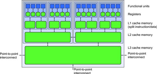
Figure 2.2 Multicore processor with hierarchical cache. Each core has multiple functional units and (typically) an instruction cache and a data cache. Larger, slower caches are then shared between increasing numbers of cores in a hierarchy.
Instruction Parallelism
Since cores usually have multiple functional units, multiple arithmetic operations can often be performed in parallel, even in a single core. Parallel use of multiple functional units in a single core can be done either implicitly, by superscalar execution of serial instructions, hardware multithreading, or by explicit vector instructions. A single-core design may use all three. A superscalar processor analyzes an instruction stream and executes multiple instructions in parallel as long as they do not depend on each other. A core with hardware multithreading supports running multiple hardware threads at the same time. There are multiple implementation approaches to this, including simultaneous multithreading, where instructions from multiple streams feed into a superscalar scheduler [TEL95, KM03], and switch-on-event multithreading, where the hardware switches rapidly to a different hardware thread when a long-latency operation, such as a memory read, is encountered [ALKK90]. Vector instructions enable explicit use of multiple functional units at once by specifying an operation on a small collection of data elements. For example, on Intel architectures vector instructions in Streaming SIMD Extension (SSE) allows specification of operations on 128-bit vectors, which can be two 64-bit values, four 32-bit values, eight 16-bit values, or sixteen 8-bit values. The new Advanced Vector Extensions (AVX) extends this feature to 256-bit vectors, and the Many Integrated Cores (MIC) architecture extends it yet again to 512-bit vectors.
Memory Hierarchy
Processors also have a memory hierarchy. Closest to the functional units are small, very fast memories known as registers. Functional units operate directly on values stored in registers. Next there are instruction and data caches. Instructions are cached separately from data at this level since their usage patterns are different. These caches are slightly slower than registers but have more space. Additional levels of cache follow, each cache level being slower but more capacious than the one above it, typically by an order of magnitude in both respects. Access to main memory is typically two orders of magnitude slower than access to the last level of cache but is much more capacious, currently up to hundreds of gigabytes on large servers. Currently, large on-chip cache memories are on the order of 10 MB, which is nonetheless a tiny sliver of the total physical memory typically available in a modern machine.
Caches are organized into blocks of storage called cache lines. A cache line is typically much larger than a single word and often (but not always) bigger than a vector. Some currently common sizes for cache lines are 64 bytes and 128 bytes. Compared with a 128-bit SSE register, which is 16 bytes wide, we see that these cache lines are 4 to 8 SSE vector registers wide. When data is read from memory, the cache is populated with an entire cache line. This allows subsequent rapid access to nearby data in the same cache line. Transferring the entire line from external memory makes it possible to amortize the overhead for setting up the transfer. On-chip, wide buses can be used to increase bandwidth between other levels of the memory hierarchy. However, if memory accesses jump around indiscriminately in memory, the extra data read into the cache goes unused. Peak memory access performance is therefore only obtained for coherent memory accesses, since that makes full use of the line transfers. Writes are usually more expensive than reads. This is because writes actually require reading the line in, modifying the written part, and (eventually) writing the line back out.
There are also two timing-related parameters to consider when discussing memory access: latency and bandwidth. Bandwidth is the amount of data that can be transferred per unit time. Latency is the amount of time that it takes to satisfy a transfer request. Latency can often be a crucial factor in performance. Random reads, for example due to “pointer chasing,” can leave the processor spending most of its time waiting for data to be returned from off-chip memory. This is a good case where hardware multithreading on a single core be beneficial, since while one thread is waiting for a memory read another can be doing computation.
Caches maintain copies of data stored elsewhere, typically in main memory. Since caches are smaller than main memory, only a subset of the data in the memory (or in the next larger cache) can be stored, and bookkeeping data needs to be maintained to keep track of where the data came from. This is the other reason for using cache lines: to amortize the cost of the bookkeeping. When an address is accessed, the caches need to be searched quickly to determine if that address’ data is in cache. A fully associative cache allows any address’ data to be stored anywhere in the cache. It is the most flexible kind of cache but expensive in hardware because the entire cache must be searched. To do this quickly, a large number of parallel hardware comparators is required.
At the other extreme are direct-mapped caches. In a direct-mapped cache, data can be placed in only one location in cache, typically using a modular function of the address. This is very simple. However, if the program happens to access two different main memory locations that map to the same location in the cache, data will get swapped into that same location repeatedly, defeating the cache. This is called a cache conflict. In a direct-mapped cache, main memory locations with conflicts are located far apart, so a conflict is theoretically rare. However, these locations are typically located at a power of two separation, so certain operations (like accessing neighboring rows in a large image whose dimensions are a power of two) can be pathological.
A set-associative cache is a common compromise between full associativity and direct mapping. Each memory address maps to a set of locations in the cache; hence, searching the cache for an address involves searching only the set it maps to, not the entire cache. Pathological cases where many accesses hit the same set can occur, but they are less frequent than for direct-mapped caches. Interestingly, a k-way set associative cache (one with k elements in each set) can be implemented using k direct-mapped caches plus a small amount of additional external hardware. Usually k is a small number, such as 4 or 8, although it is as large as 16 on some recent Intel processors.
Caches further down in the hierarchy are typically also shared among an increasing number of cores. Special hardware keeps the contents of caches consistent with one another. When cores communicate using “shared memory,” they are often really just communicating through the cache coherence mechanisms. Another pathological case can occur when two cores access data that happens to lie in the same cache line. Normally, cache coherency protocols assign one core, the one that last modifies a cache line, to be the “owner” of that cache line. If two cores write to the same cache line repeatedly, they fight over ownership. Importantly, note that this can happen even if the cores are not writing to the same part of the cache line. This problem is called false sharing and can significantly decrease performance. In particular, as noted in Section 2.3, this leads to a significant difference in the benefit of memory coherence in threads and vector mechanisms for parallelism.
Virtual Memory
Virtual memory lets each processor use its own logical address space, which the hardware maps to the actual physical memory. The mapping is done per page, where pages are relatively large blocks of memory, on the order of 4 KB to 16 KB. Virtual memory enables running programs with larger data sets than would fit in physical memory. Parts of the virtual memory space not in active use are kept in a disk file called a swap file so the physical memory can be remapped to other local addresses in use. In a sense, the main memory acts as cache for the data stored on disk. However, since disk access latency is literally millions of times slower than memory access latency, a page fault—an attempt to access a location that is not in physical memory—can take a long time to resolve. If the page fault rate is high, then performance can suffer. Originally, virtual memory was designed for the situation in which many users were time-sharing a computer. In this case, applications would be “swapped out” when a user was not active, and many processes would be available to hide latency. In other situations, virtual memory may not be able to provide the illusion of a large memory space efficiently, but it is still useful for providing isolation between processes and simplifying memory allocation.
Generally speaking, data locality is important at the level of virtual memory for two reasons. First, good performance requires that the page fault rate be low. This means that the ordering of accesses to data should be such that the working set of the process—the total amount of physical memory that needs to be accessed within a time period that is short relative to the disk access time—should fit in the set of physical memory pages that can be assigned to the process. Second, addresses must be translated rapidly from virtual addresses to physical addresses. This is done by specialized hardware called a Translation Lookaside Buffer (TLB). The TLB is a specialized cache that translates logical addresses to physical addresses for a small set of active pages. Like ordinary caches, it may have hierarchical levels and may be split for instructions versus data. If a memory access is made to a page not currently in the TLB, then a TLB miss occurs. A TLB miss requires walking a page table in memory to find the translation. The walk is done by either specialized hardware or a trap to the operating system. Since the TLB is finite, updating the TLB typically requires the eviction of some other translation entry.
The important issue is that the number of page translation entries in the TLB is relatively small, on the order of 8 to 128 entries for the first-level TLB, and TLB misses, while not as expensive as page faults, are not cheap. Therefore, accessing a large number of pages in a short timeframe can cause TLB thrashing, a high TLB miss rate that can significantly degrade performance.
A typical case for this issue is a stencil on a large 3D array. Suppose a program sweeps through the array in the obvious order—row, column, page—accessing a stencil of neighboring elements for each location. If the number of pages touched by a single row sweep is larger than the size of the TLB, this will tend to cause a high TLB miss rate. This will be true even if the page fault rate is low. Of course, if the 3D array is big enough, then a high page fault rate might also result. Reordering the stencil to improve locality (for example, as in Chapter 10) can lower the TLB miss rate and improve performance. Another way to address this is to use large pages so that a given number of TLB entries can cover a larger amount of physical memory. Some processors partition the TLB into portions for small and large pages, so that large pages can be used where beneficial, and not where they would do more harm than good.
Multiprocessor Systems
Processors may be combined together to form multiple-processor systems. In modern systems, this is done by attaching memory directly to each processor and then connecting the processors (or actually, their caches) with fast point-to-point communications channels, as in Figure 2.3. The cache coherency protocol is extended across these systems, and processors can access memory attached to other processors across the communication channels.
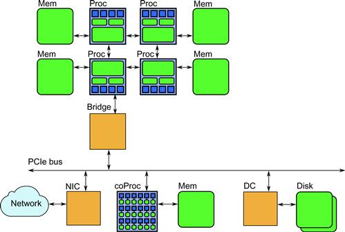
Figure 2.3 Multiprocessor system organization. Each processor has its own memory bank(s), and processors are interconnected using point-to-point communication channels. A processor can access its own memory directly and other banks over the communication channels. A bridge chip connects the processors to other devices, often through a bus such as a PCIe bus. Communication devices (Network Interface Controllers, or NICs) and other processors (GPUs or attached co-processors) can be attached to the PCIe bus (actually, the PCIe bus is not an actual shared bus but another set of point-to-point data links).
However, access to memory attached to a remote processor is slower (has higher latency and also typically reduced bandwidth) than access to a local memory. This results in non-uniform memory access (NUMA). Ideally, threads should be placed on cores close to the data they should process, or vice versa. The effect is not large for machines with a small number of processors but can be pronounced for large-scale machines. Because NUMA also affects cache coherency, other problems, such as false sharing, can be magnified in multiprocessor machines.
One basic theoretical model of parallel computation, the Parallel Random Access Machine (PRAM), assumes uniform memory-access times for simplicity, and there have been attempts to build real machines like this [Vis11]. However, both caching and NUMA invalidate this assumption. Caches make access time depend on previous accesses, and NUMA makes access time depend on the location of data. The constants involved are not small, either. Access to main memory can be hundreds of times slower than access to cache. Designing algorithms to have good cache behavior is important for serial programs, but becomes even more important for parallel programs.
Theoretical models that extend PRAM to quantify overhead of interprocessor communication include the Synchronous Parallel (BSP) [Val90] and the LogP [CKP+96] models.
Attached Devices
Other devices are often attached to the processor. For example, a PCIe bus allows devices to be installed by end users. A Network Interface Controller (NIC) is a typical PCIe device that provides access to the network. High-performance NICs can require high bandwidth and additionally the overall system performance of a cluster can depend crucially on communication latency. The PCIe bus protocol allows for such devices to perform direct memory access (DMA) and read or write data directly to memory, without involving the main processor (except for coordination).
Other devices with high memory requirements may also use DMA. Such devices included attached processing units such as graphics accelerators and many-core processors.
Such co-processors can be quite sophisticated systems in their own right. The Intel Many Integrated Core (MIC) architecture, for example, is a high-performance processor with a large number of simple cores (over 50) and its own cache and memory system. Each MIC core also has wide vector units, 512 bits, which is twice as wide as AVX. These characteristics make it more suitable for highly parallelizable and vectorizable workloads with regular data parallelism than multicore processors, which are optimized for high scalar performance.
While the main function of graphics accelerators is the generation of images, they can also be used to provide supplemental processing power, since they also have wide vector units and many cores. Graphics accelerators used as computational engines are usually programmed using the SIMT model discussed in Section 2.4.3 through a programming model such as OpenCL or (for graphics accelerators from NVIDIA) CUDA.
However, while graphics accelerators must be programmed with a specialized programming model such as OpenCL, the Intel MIC architecture runs a full operating system (Linux) and can be programmed with nearly any parallel programming model available on multicore processors. This includes (but is not limited to) all the programming models discussed in this book.
2.4.2 Key Features for Performance
Given the complexities of computer architecture, and the fact that different computers can vary significantly, how can you optimize code for performance across a range of computer architectures?
The trick is to realize that modern computer architectures are designed around two key assumptions: data locality and the availability of parallel operations. Get these right and good performance can be achieved on a wide range of machines, although perhaps after some per-machine tuning. However, if you violate these assumptions, you cannot expect good performance no matter how much low-level tuning you do. In this section, we will also discuss some useful strategies for avoiding dependence on particular machine configurations: cache oblivious algorithms and parameterized code.
Data Locality
Good use of memory bandwidth and good use of cache depends on good data locality, which is the reuse of data from nearby locations in time or space. Therefore, you should design your algorithms to have good data locality by using one or more of the following strategies:
• Break work up into chunks that can fit in cache. If the working set for a chunk of work does not fit in cache, it will not run efficiently.
• Organize data structures and memory accesses to reuse data locally when possible. Avoid unnecessary accesses far apart in memory and especially simultaneous access to multiple memory locations located a power of two apart. The last consideration is to avoid cache conflicts on caches with low associativity.
• To avoid unnecessary TLB misses, avoid accessing too many pages at once.
• Align data with cache line boundaries. Avoid having unrelated data accesses from different cores access the same cache lines, to avoid false sharing.
Some of these may require changes to data layout, including reordering items and adding padding to achieve (or avoid) alignments with the hardware architecture. Not only is breaking up work into chunks and getting good alignment with the cache good for parallelization but these optimizations can also make a big difference to single-core performance.
However, these guidelines can be hard to follow when writing portable code, since then you have no advance knowledge of the cache line sizes, the cache organization, or the total size of the caches. In this case, use memory allocation routines that can be customized to the machine, and parameterize your code so that the grain size (the size of a chunk of work) can be selected dynamically. If code is parameterized in this way, then when porting to a new machine the tuning process will involve only finding optimal values for these parameters rather than re-coding. If the search for optimal parameters is done automatically it is known as autotuning, which may also involve searching over algorithm variants as well.
Another approach to tuning grain size is to design algorithms so that they have locality at all scales, using recursive decomposition. This so-called cache oblivious approach avoids the need to know the size or organization of the cache to tune the algorithm. Section 8.8 says more about the cache oblivious approach.
Another issue that affects the achievable performance of an algorithm is arithmetic intensity. This is the ratio of computation to communication. Given the fact that on-chip compute performance is still rising with the number of transistors, but off-chip bandwidth is not rising as fast, in order to achieve scalability approaches to parallelism should be sought that give high arithmetic intensity. This ideally means that a large number of on-chip compute operations should be performed for every off-chip memory access. Throughout this book we discuss several optimizations that are aimed at increasing arithmetic intensity, including fusion and tiling.
Sometimes there is conflict between small grain sizes (which give high parallelism) and high arithmetic intensity. For example, in a 2D recurrence tiling (discussed in Chapter 7), the amount of work in a tile might grow as Θ(n2) while the communication grows as Θ(n). In this case the arithmetic intensity grows by ![]() , which favors larger grain sizes. In practice, the largest grain size that still fits in cache will likely give the best performance with the least overhead. However, a large grain size may also reduce the available parallelism (“parallel slack”) since it will reduce the total number of work units.
, which favors larger grain sizes. In practice, the largest grain size that still fits in cache will likely give the best performance with the least overhead. However, a large grain size may also reduce the available parallelism (“parallel slack”) since it will reduce the total number of work units.
Parallel Slack
Parallel slack is the amount of “extra” parallelism available (Section 2.5.6) above the minimum necessary to use the parallel hardware resources. Specifying a significant amount of potential parallelism higher than the actual parallelism of the hardware gives the underlying software and hardware schedulers more flexibility to exploit machine resources.
Normally you want to choose the smallest work units possible that reasonably amortize the overhead of scheduling them and give good arithmetic intensity. Breaking down a problem into exactly as many chunks of work as there are cores available on the machine is tempting, but not necessarily optimal, even if you know the number of cores on the machine. If you only have one or a few tasks on each core, then a delay on one core (perhaps due to an operating system interrupt) is likely to delay the entire program.
Having lots of parallel slack works well with the Intel Cilk Plus and Intel TBB task schedulers because they are designed to exploit slack. In contrast when using OS threading interfaces such as POSIX threads, too much actual parallelism can be detrimental. This problem often does not happen on purpose but due to nesting parallelism using direct threading. Suppose on a 16-core system that an algorithm f creates 15 extra threads to assist its calling thread, and each thread calls a library routine g. If the implementer of g applies the same logic, now there are 16 × 15 threads running concurrently! Because these threads have mandatory concurrency semantics (they must run in parallel), the OS must time-slice execution among all 240 threads, incurring overhead for context switching and reloading items into cache. Using tasks instead is better here, because tasks have semantics that make actual parallelism optional. This enables the task scheduler to automatically match actual parallelism to the hardware capability, even when parallelism is nested or irregular.
As mentioned earlier, having more potential parallelism than cores can also help performance when the cores support hardware multithreading. For example, if pointer-chasing code using dependent memory reads cannot be avoided, then additional parallelism can enable hardware-multithreading to hide the latency of the memory reads. However, if additional parallelism is used for this purpose, the total working set needs to be considered so that the cache size is not exceeded for all concurrently active threads. If parallelism is increased for this purpose, the grain size might have to be reduced for best performance.
2.4.3 Flynn’s Characterization
One way to coarsely characterize the parallelism available in processor types is by how they combine control flow and data management. A classic categorization by Flynn [Fly72] divides parallel processors into categories based on whether they have multiple flows of control, multiple streams of data, or both.
• Single Instruction, Single Data (SISD): This is just a standard non-parallel processor. We usually refer to this as a scalar processor. Due to Amdahl’s Law (discussed in Section 2.5.4), the performance of scalar processing is important; if it is slow it can end up dominating performance.
• Single Instruction, Multiple Data (SIMD): A single operation (task) executes simultaneously on multiple elements of data. The number of elements in a SIMD operation can vary from a small number, such as the 4 to 16 elements in short vector instructions, to thousands, as in streaming vector processors. SIMD processors are also known as array processors, since they consist of an array of functional units with a shared controller.
• Multiple Instruction, Multiple Data (MIMD): Separate instruction streams, each with its own flow of control, operate on separate data. This characterizes the use of multiple cores in a single processor, multiple processors in a single computer, and multiple computers in a cluster. When multiple processors using different architectures are present in the same computer system, we say it is a heterogeneous computer. An example would be a host processor and a co-processor with different instruction sets.
The last possible combination, MISD, is not particularly useful and is not used.
Another way often used to classify computers is by whether every processor can access a common shared memory or if each processor can only access memory local to it. The latter case is called distributed memory. Many distributed memory systems have local shared-memory subsystems. In particular, clusters are large distributed-memory systems formed by connecting many shared-memory computers (“nodes”) with a high-speed communication network. Clusters are formed by connecting otherwise independent systems and so are almost always MIMD systems. Often shared-memory computers really do have physically distributed memory systems; it’s just that the communication used to create the illusion of shared memory is implicit.
There is another related classification used especially by GPU vendors: Single Instruction, Multiple Threads (SIMT). This corresponds to a tiled SIMD architecture consisting of multiple SIMD processors, where each SIMD processor emulates multiple “threads” (fibers in our terminology) using masking. SIMT processors may appear to have thousands of threads, but in fact blocks of these share a control processor, and divergent control flow can significantly reduce efficiency within a block. On the other hand, synchronization between fibers is basically free, because when control flow is emulated with masking the fibers are always running synchronously.
Memory access patterns can also affect the performance of a processor using the SIMT model. Typically each SIMD subprocessor in a SIMT machine is designed to use the data from a cache line. If memory access from different fibers access completely different cache lines, then performance drops since often the processor will require multiple memory cycles to resolve the memory access. These are called divergent memory accesses. In contrast, if all fibers in a SIMD core access the same cache lines, then the memory accesses can be coalesced and performance improved. It is important to note that this is exactly the opposite of what we want to do if the fibers really were separate threads. If the fibers were running on different cores, then we want to avoid having them access the same cache line. Therefore, while code written to use fibers may be implemented using hardware threads on multiple cores, code properly optimized for fibers will actually be suboptimal for threads when it comes to memory access.
2.4.4 Evolution
Predictions are very difficult, especially about the future.
(Niels Bohr)
Computers continue to evolve, although the fundamentals of parallelism and data locality will continue to be important. An important recent trend is the development of attached processing such as graphics accelerators and co-processors specialized for highly parallel workloads.
Graphics accelerators are also known as GPUs. While originally designed for graphics, GPUs have become general-purpose enough to be used for other computational tasks.
In this book we discuss, relatively briefly, a standard language and application programming interface (API) called OpenCL for programming many-core devices from multiple vendors, including GPUs. GPUs from NVIDIA can also be programmed with a proprietary language called CUDA. For the most part, OpenCL replicates the functionality of CUDA but provides the additional benefit of portability. OpenCL generalizes the idea of computation on a GPU to computation on multiple types of attached processing. With OpenCL, it is possible to write a parallel program that can run on the main processor, on a co-processor, or on a GPU. However, the semantic limitations of the OpenCL programming model reflect the limitations of GPUs.
Running computations on an accelerator or co-processor is commonly referred to as offload. As an alternative to OpenCL or CUDA, several compilers (including the Intel compiler) now support offload pragmas to move computations and data to an accelerator or co-processor with minimal code changes. Offload pragmas allow annotating the original source code rather than rewriting the “kernels” in a separate language, as with OpenCL. However, even with an offload pragma syntax, any code being offloaded still has to fit within the semantic limitations of the accelerator or co-processor to which it is being offloaded. Limitations of the target may force multiple versions of code. For example, if the target processor does not support recursion or function pointers, then it will not be possible to offload code that uses these language features to that processor. This is true even if the feature is being used implicitly. For example, the “virtual functions” used to support C++ class inheritance use function pointers in their implementation. Without function pointer support in the target hardware it is therefore not possible to offload general C++ code.
Some tuning of offloaded code is also usually needed, even if there is a semantic match. For example, GPUs are designed to handle large amounts of fine-grained parallelism with relatively small working sets and high coherence. Unlike traditional general-purpose CPUs, they have relatively small on-chip memories and depend on large numbers of active threads to hide latency, so that data can be streamed in from off-chip memory. They also have wide vector units and simulate many fibers (pseudo-threads) at once using masking to emulate control flow.
These architectural choices can be good tradeoffs for certain types of applications, which has given rise to the term heterogeneous computing: the idea that different processor designs are suitable for different kinds of workloads, so a computer should include multiple cores of different types. This would allow the most efficient core for a given application, or stage of an application, to be used. This concept can be extended to even more specialized hardware integrated into a processor, such as video decoders, although usually it refers to multiple types of programmable processor.
GPUs are not the only offload device available. It is also possible to use programmable hardware such as field programmable gate arrays (FPGAs) and co-processors made of many-core processors, such as the Intel MIC (Many Integrated Cores) architecture. While the MIC architecture can be programmed with OpenCL, it is also possible to use standard CPU programming models with it. However, the MIC architecture has many more cores than most CPUs (over 50), and each core has wide vector units (16 single-precision floats). This is similar in some ways to GPU architectures and enables high peak floating point performance. The tradeoff is that cache size per core is reduced, so it is even more important to have good data locality in implementations.
However, the main difference between MIC and GPUs is in the variety of programming models supported: The MIC is a general-purpose processor running a standard operating system (Linux) with full compiler support for C, C++, and Fortran. It also appears as a distributed-memory node on the network. The MIC architecture is therefore not limited to OpenCL or CUDA but can use any programming model (including, for instance, MPI) that would run on a mainstream processor. It also means that offload pragma syntax does not have to be limited by semantic differences between the host processor and the target processor.
Currently, GPUs are primarily available as discrete devices located on the PCIe bus and do not share memory with the host. This is also the current model for the MIC co-processor. However, this model has many inefficiencies, since data must be transferred across the PCIe bus to a memory local to the device before it can be processed.
As another possible model for integrating accelerators or co-processors within a computer system, GPUs cores with their wide vector units have been integrated into the same die as the main processor cores by both AMD and Intel. NVIDIA also makes integrated CPU/GPU processors using ARM main cores for the embedded and mobile markets. For these, physical memory is shared by the GPU and CPU processors. Recently, APIs and hardware support have been rapidly evolving to allow data sharing without copying. This approach will allow much finer-grained heterogeneous computing, and processors may in fact evolve so that there are simply multiple cores with various characteristics on single die, not separate CPUs, GPUs, and co-processors.
Regardless of whether a parallel program is executed on a CPU, a GPU, or a many-core co-processor, the basic requirements are the same: Software must be designed for a high level of parallelism and with good data locality. Ultimately, these processor types are not that different; they just represent different points on a design spectrum that vary in the programming models they can support most efficiently.
2.5 Performance Theory
The primary purpose of parallelization, as discussed in this book, is performance. So what is performance? Usually it is about one of the following:
• Reducing the total time it takes to compute a single result (latency; Section 2.5.1)
• Increasing the rate at which a series of results can be computed (throughput; Section 2.5.1)
• Reducing the power consumption of a computation (Section 2.5.3)
All these valid interpretations of “performance” can be achieved by parallelization.
There is also a distinction between improving performance to reduce costs or to meet a deadline. To reduce costs, you want to get more done within a fixed machine or power budget and usually are not willing to increase the total amount of computational work. Alternatively, to meet a deadline, you might be willing to increase the total amount of work if it means the jobs gets done sooner. For instance, in an interactive application, you might need to complete work fast enough to meet a certain frame rate or response time. In this case, extra work such as redundant or speculative computation might help meet the deadline. Choose such extra work with care, since it may actually decrease performance, as discussed in Section 2.5.6.
Once you have defined a performance target, then generally you should iteratively modify an application to improve its performance until the target is reached. It is important during this optimization process to start from a working implementation and validate the results after every program transformation. Fast computation of wrong answers is pointless, so continuous validation is strongly recommended to avoid wasting time tuning a broken implementation.
Validation should be given careful thought, in light of the original purpose of the program. Obtaining results “bit identical” to the serial program is sometimes unrealistic if the algorithm needs to be modified to support parallelization. Indeed, the parallel program’s results, though different, may be as as good for the overall purpose as the original serial program, or even better.
During the optimization process you should measure performance to see if you are making progress. Performance can be measured empirically on real hardware or estimated using analytic models based on ideal theoretical machines. Both approaches are valuable. Empirical measures account for real-world effects but often give little insight into root causes and therefore offer little guidance as to how performance could be improved or why it is limited. Analytic measures, particularly the work-span model explained in Section 2.5.6, ignore some real-world effects but give insight into the fundamental scaling limitations of a parallel algorithm. Analytic approaches also allow you to compare parallelization strategies at a lower cost than actually doing an implementation. We recommend using analytic measures to guide selection of an algorithm, accompanied by “back of the envelope” estimates of plausibility. After an algorithm is implemented, use empirical measures to understand and deal with effects ignored by the analytic model.
2.5.1 Latency and Throughput
The time it takes to complete a task is called latency. It has units of time. The scale can be anywhere from nanoseconds to days. Lower latency is better.
The rate a which a series of tasks can be completed is called throughput. This has units of work per unit time. Larger throughput is better. A related term is bandwidth, which refers to throughput rates that have a frequency-domain interpretation, particularly when referring to memory or communication transactions.
Some optimizations that improve throughput may increase the latency. For example, processing of a series of tasks can be parallelized by pipelining, which overlaps different stages of processing. However, pipelining adds overhead since the stages must now synchronize and communicate, so the time it takes to get one complete task through the whole pipeline may take longer than with a simple serial implementation.
Related to latency is response time. This measure is often used in transaction processing systems, such as web servers, where many transactions from different sources need to be processed. To maintain a given quality of service each transaction should be processed in a given amount of time. However, some latency may be sacrificed even in this case in order to improve throughput. In particular, tasks may be queued up, and time spent waiting in the queue increases each task’s latency. However, queuing tasks improves the overall utilization of the computing resources and so improves throughput and reduces costs.
“Extra” parallelism can also be used for latency hiding. Latency hiding does not actually reduce latency; instead, it improves utilization and throughput by quickly switching to another task whenever one task needs to wait for a high-latency activity. Section 2.5.9 says more about this.
2.5.2 Speedup, Efficiency, and Scalability
Two important metrics related to performance and parallelism are speedup and efficiency. Speedup compares the latency for solving the identical computational problem on one hardware unit (“worker”) versus on P hardware units:
![]() (2.1)
(2.1)
where T1 is the latency of the program with one worker and TP is the latency on P workers.
Efficiency is speedup divided by the number of workers:
![]() (2.2)
(2.2)
Efficiency measures return on hardware investment. Ideal efficiency is 1 (often reported as 100%), which corresponds to a linear speedup, but many factors can reduce efficiency below this ideal.
If T1 is the latency of the parallel program running with a single worker, Equation 2.1 is sometimes called relative speedup, because it shows relative improvement from using P workers. This uses a serialization of the parallel algorithm as the baseline. However, sometimes there is a better serial algorithm that does not parallelize well. If so, it is fairer to use that algorithm for T1, and report absolute speedup, as long as both algorithms are solving an identical computational problem. Otherwise, using an unnecessarily poor baseline artificially inflates speedup and efficiency.
In some cases, it is also fair to use algorithms that produce numerically different answers, as long as they solve the same problem according to the problem definition. In particular, reordering floating point computations is sometimes unavoidable. Since floating point operations are not truly associative, reordering can lead to differences in output, sometimes radically different if a floating point comparison leads to a divergence in control flow. Whether the serial or parallel result is actually more accurate depends on the circumstances.
Speedup, not efficiency, is what you see in advertisements for parallel computers, because speedups can be large impressive numbers. Efficiencies, except in unusual circumstances, do not exceed 100% and often sound depressingly low. A speedup of 100 sounds better than an efficiency of 10%, even if both are for the same program and same machine with 1000 cores.
An algorithm that runs P times faster on P processors is said to exhibit linear speedup. Linear speedup is rare in practice, since there is extra work involved in distributing work to processors and coordinating them. In addition, an optimal serial algorithm may be able to do less work overall than an optimal parallel algorithm for certain problems, so the achievable speedup may be sublinear in P, even on theoretical ideal machines. Linear speedup is usually considered optimal since we can serialize the parallel algorithm, as noted above, and run it on a serial machine with a linear slowdown as a worst-case baseline.
However, as exceptions that prove the rule, an occasional program will exhibit superlinear speedup—an efficiency greater than 100%. Some common causes of superlinear speedup include:
• Restructuring a program for parallel execution can cause it to use cache memory better, even when run on with a single worker! But if T1 from the old program is still used for the speedup calculation, the speedup can appear to be superlinear. See Section 10.5 for an example of restructuring that often reduces T1 significantly.
• The program’s performance is strongly dependent on having a sufficient amount of cache memory, and no single worker has access to that amount. If multiple workers bring that amount to bear, because they do not all share the same cache, absolute speedup really can be superlinear.
• The parallel algorithm may be more efficient than the equivalent serial algorithm, since it may be able to avoid work that its serialization would be forced to do. For example, in search tree problems, searching multiple branches in parallel sometimes permits chopping off branches (by using results computed in sibling branches) sooner than would occur in the serial code.
However, for the most part, sublinear speedup is the norm.
Section 2.5.4 discusses an important limit on speedup: Amdahl’s Law. It considers speedup as P varies and the problem size remains fixed. This is sometimes called strong scalability. Section 2.5.5 discusses an alternative, Gustafson-Barsis’ Law, which assumes the problem size grows with P. This is sometimes called weak scalability. But before discussing speedup further, we discuss another motivation for parallelism: power.
2.5.3 Power
Parallelization can reduce power consumption. CMOS is the dominant circuit technology for current computer hardware. CMOS power consumption is the sum of dynamic power consumption and static power consumption [VF05]. For a circuit supply voltage V and operating frequency f, CMOS dynamic power dissipation is governed by the proportion
![]()
The frequency dependence is actually more severe than the equation suggests, because the highest frequency at which a CMOS circuit can operate is roughly proportional to the voltage. Thus dynamic power varies as the cube of the maximum frequency. Static power consumption is nominally independent of frequency but is dependent on voltage. The relation is more complex than for dynamic power, but, for sake of argument, assume it varies cubically with voltage. Since the necessary voltage is proportional to the maximum frequency, the static power consumption varies as the cube of the maximum frequency, too. Under this assumption we can use a simple overall model where the total power consumption varies by the cube of the frequency.
Suppose that parallelization speeds up an application by 1.5× on two cores. You can use this speedup either to reduce latency or reduce power. If your latency requirement is already met, then reducing the clock rate of the cores by 1.5× will save a significant amount of power. Let ![]() be the power consumed by one core running the serial version of the application. Then the power consumed by two cores running the parallel version of the application will be given by:
be the power consumed by one core running the serial version of the application. Then the power consumed by two cores running the parallel version of the application will be given by:
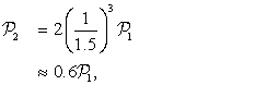
where the factor of 2 arises from having two cores. Using two cores running the parallelized version of the application at the lower clock rate has the same latency but uses (in this case) 40% less power.
Unfortunately, reality is not so simple. Current chips have so many transistors that frequency and voltage are already scaled down to near the lower limit just to avoid overheating, so there is not much leeway for raising the frequency. For example, Intel Turbo Boost Technology enables cores to be put to sleep so that the power can be devoted to the remaining cores while keeping the chip within its thermal design power limits. Table 2.1 shows an example. Still, the table shows that even low parallel efficiencies offer more performance on this chip than serial execution.
Table 2.1. Running Fewer Cores Faster [Cor11c]. The table shows how the maximum core frequency for an Intel core i5-2500T chip depends on the number of active cores. The last column shows the parallel efficiency over all four cores required to match the speed of using only one active core.
| Active Cores | Maximum Frequency (GHz) | Breakeven Efficiency |
| 4 | 2.4 | 34% |
| 3 | 2.8 | 39% |
| 2 | 3.2 | 52% |
| 1 | 3.3 | 100% |
Another way to save power is to “race to sleep” [DHKC09]. In this strategy, we try to get the computation done as fast as possible (with the lowest latency) so that all the cores can be put in a sleep state that draws very little power. This approach is attractive if a significant fraction of the wakeful power is fixed regardless of how many cores are running.
Especially in mobile devices, parallelism can be used to reduce latency. This reduces the time the device, including its display and other components, is powered up. This not only improves the user experience but also reduces the overall power consumption for performing a user’s task: a win-win.
2.5.4 Amdahl’s Law
… the effort expended on achieving high parallel processing rates is wasted unless it is accompanied by achievements in sequential processing rates of very nearly the same magnitude.
(Gene Amdahl [Amd67])
Amdahl argued that the execution time T1 of a program falls into two categories:
Call these Wser and Wpar, respectively. Given P workers available to do the parallelizable work, the times for sequential execution and parallel execution are:
![]()
The bound on TP assumes no superlinear speedup, and is an exact equality only if the parallelizable work can be perfectly parallelized. Plugging these relations into the definition of speedup yields Amdahl’s Law:
![]() (2.3)
(2.3)
Figure 2.4 visualizes this bound.
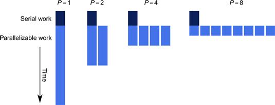
Figure 2.4 Amdahl’s Law. Speedup is limited by the non-parallelizable serial portion of the work.
Amdahl’s Law has an important corollary. Let f be the non-parallelizable serial fraction of the total work. Then the following equalities hold:
![]()
Substitute these into Equation 2.3 and simplify to get:
![]() (2.4)
(2.4)
Now consider what happens when P tends to infinity:
![]() (2.5)
(2.5)
Speedup is limited by the fraction of the work that is not parallelizable, even using an infinite number of processors. If 10% of the application cannot be parallelized, then the maximum speedup is 10×. If 1% of the application cannot be parallelized, then the maximum speedup is 100×. In practice, an infinite number of processors is not available. With fewer processors, the speedup may be reduced, which gives an upper bound on the speedup. Amdahl’s Law is graphed in Figure 2.5, which shows the bound for various values of f and P. For example, observe that even with f = 0.001 (that is, only 0.1% of the application is serial) and P = 2048, a program’s speedup is limited to 672×. This limitation on speedup can also be viewed as inefficient use of parallel hardware resources for large serial fractions, as shown in Figure 2.6.
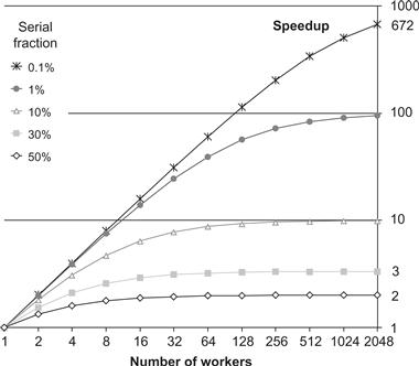
Figure 2.5 Amdahl’s Law: speedup. The scalability of parallelization is limited by the non-parallelizable (serial) portion of the workload. The serial fraction is the percentage of code that is not parallelized.
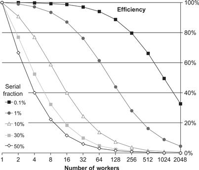
Figure 2.6 Amdahl’s Law: efficiency. Even when speedups are possible, the efficiency can easily become poor. The serial fraction is the percentage of code that is not parallelized.
2.5.5 Gustafson-Barsis’ Law
… speedup should be measured by scaling the problem to the number of processors, not by fixing the problem size.
(John Gustafson [Gus88])
Amdahl’s Law views programs as fixed and the computer as changeable, but experience indicates that as computers get new capabilities, applications change to exploit these features. Most of today’s applications would not run on computers from 10 years ago, and many would run poorly on machines that are just 5 years old. This observation is not limited to obvious applications such as games; it applies also to office applications, web browsers, photography software, DVD production and editing software, and Google Earth.
More than two decades after the appearance of Amdahl’s Law, John Gustafson2 noted that several programs at Sandia National Labs were speeding up by over 1000×. Clearly, Amdahl’s Law could be evaded.
Gustafson noted that problem sizes grow as computers become more powerful. As the problem size grows, the work required for the parallel part of the problem frequently grows much faster than the serial part. If this is true for a given application, then as the problem size grows the serial fraction decreases and speedup improves.
Figure 2.7 visualizes this using the assumption that the serial portion is constant while the parallel portion grows linearly with the problem size. On the left is the application running with one worker. As workers are added, the application solves bigger problems in the same time, not the same problem in less time. The serial portion still takes the same amount of time to perform, but diminishes as a fraction of the whole. Once the serial portion becomes insignificant, speedup grows practically at the same rate as the number of processors, thus achieving linear speedup.
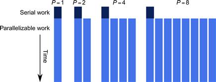
Figure 2.7 Gustafson-Barsis’ Law. If the problem size increases with P while the serial portion grows slowly or remains fixed, speedup grows as workers are added.
Both Amdahl’s and Gustafson-Barsis’ Laws are correct. It is a matter of “glass half empty” or “glass half full.” The difference lies in whether you want to make a program run faster with the same workload or run in the same time with a larger workload. History clearly favors programs getting more complex and solving larger problems, so Gustafson’s observations fit the historical trend. Nevertheless, Amdahl’s Law still haunts you when you need to make an application run faster on the same workload to meet some latency target.
Furthermore, Gustafson-Barsis’ observation is not a license for carelessness. In order for it to hold it is critical to ensure that serial work grows much more slowly than parallel work, and that synchronization and other forms of overhead are scalable.
2.5.6 Work-Span Model
This section introduces the work-span model for parallel computation. The work-span model is much more useful than Amdahl’s law for estimating program running times, because it takes into account imperfect parallelization. Furthermore, it is not just an upper bound as it also provides a lower bound. It lets you estimate TP from just two numbers: T1 and T∞.
In the work-span model, tasks form a directed acyclic graph. A task is ready to run if all of its predecessors in the graph are done. The basic work-span model ignores communication and memory access costs. It also assumes task scheduling is greedy, which means the scheduler never lets a hardware worker sit idle while there is a task ready to run.
The extreme times for P = 1 and P = ∞ are so important that they have names. Time T1 is called the work of an algorithm. It is the time that a serialization of the algorithm would take and is simply the total time it would take to complete all tasks. Time T∞ is called the span of an algorithm. The span is the time a parallel algorithm would take on an ideal machine with an infinite number of processors. Span is equivalent to the length of the critical path. The critical path is the longest chain of tasks that must be executed one after each other. Synonyms for span in the literature are step complexity or depth.
Figure 2.8 shows an example. Each box represents a task taking unit time, with arrows showing dependencies. The work is 18, because there are 18 tasks. The span is 6, because the longest chain of tasks that must be evaluated one after the other contains 6 tasks.
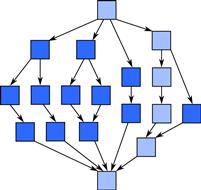
Figure 2.8 Work and span. Arrows denote dependencies between tasks. Work is the total amount of computation, while span is given by the critical path. In this example, if each task takes unit time, the work is 18 and the span is 6.
Work and span each put a limit on speedup. Superlinear speedup is impossible in the work-span model:
![]() (2.6)
(2.6)
On an ideal machine with greedy scheduling, adding processors never slows down an algorithm:
![]() (2.7)
(2.7)
Or more colloquially:
![]()
For example, the speedup for Figure 2.8 can never exceed 3, because ![]() . Real machines introduce synchronization overhead, not only for the synchronization constructs themselves, but also for communication. A span that includes these overheads is called a burdened span [HLL10].
. Real machines introduce synchronization overhead, not only for the synchronization constructs themselves, but also for communication. A span that includes these overheads is called a burdened span [HLL10].
The span provides more than just an upper bound on speedup. It can also be used to estimate a lower bound on speedup for an ideal machine. An inequality known as Brent’s Lemma [Bre74] bounds TP in terms of the work T1 and the span T∞:
![]() (2.8)
(2.8)
Here is the argument behind the lemma. The total work T1 can be divided into two categories: perfectly parallelizable work and imperfectly parallelizable work. The imperfectly parallelizable work takes time T∞ no matter how many workers there are. The perfectly parallelizable work remaining takes time T1 − T∞ with a single worker, and since it is perfectly parallelizable it speeds up by P if all P workers are working on it. But if not all P workers are working on it, then at least one worker is working on the T∞ component. The argument resembles Amdahl’s argument, but generalizes the notion of an inherently serial portion of work to imperfectly parallelizable work.
Though the argument resembles Amdahl’s argument, it proves something quite different. Amdahl’s argument put a lower bound on TP and is exact only if the parallelizable portion of a program is perfectly parallelizable. Brent’s Lemma puts an upper bound on TP. It says what happens if the worst possible assignment of tasks to workers is chosen.
In general, work-span analysis is a far better guide than Amdahl’s Law, because it usually provides a tighter upper bound and also provides a lower bound. Figure 2.9 compares the bounds given by Amdahl’s Law and work-span analysis for the task graph in Figure 2.8. There are 18 tasks. The first and last tasks constitute serial work; the other tasks constitute parallelizable work. Hence, the fraction of serial work is ![]() . By Amdahl’s Law, the limit on speedup is 9. Work-span analysis says the speedup is limited by the
. By Amdahl’s Law, the limit on speedup is 9. Work-span analysis says the speedup is limited by the ![]() , which is at most 3, a third of what Amdahl’s law indicates. The difference is that the work-span analysis accounted for how parallelizable the parallel work really is. The bottom curve in the figure is the lower bound provided by Brent’s lemma. It says, for example, that with 4 workers a speedup of 2 is guaranteed, no matter how the tasks are assigned to workers.
, which is at most 3, a third of what Amdahl’s law indicates. The difference is that the work-span analysis accounted for how parallelizable the parallel work really is. The bottom curve in the figure is the lower bound provided by Brent’s lemma. It says, for example, that with 4 workers a speedup of 2 is guaranteed, no matter how the tasks are assigned to workers.
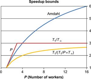
Figure 2.9 Amdahl was an optimist. Using the work and span of Figure 2.8, this graph illustrates that the upper bound by Amdahl’s Law is often much higher than what work-span analysis reveals. Furthermore, work-span analysis provides a lower bound for speedup, too, assuming greedy scheduling on an ideal machine.
Brent’s Lemma leads to a useful formula for estimating TP from the work T1 and span T∞. To get much speedup, T1 must be significantly larger than T∞, In this case, ![]() and the right side of 2.8 also turns out to be a good lower bound estimate on TP. So the following approximation works well in practice for estimating running time:
and the right side of 2.8 also turns out to be a good lower bound estimate on TP. So the following approximation works well in practice for estimating running time:
![]() (2.9)
(2.9)
When designing a parallel algorithm, avoid creating significantly more work for the sake of parallelization, and focus on reducing the span, because the span is the fundamental asymptotic limit on scalability. Increase the work only if it enables a drastic decrease in span. An example of this is the scan pattern, where the span can be reduced from linear to logarithmic complexity by doubling the work (Section 8.11).
Brent’s Lemma also leads to a formal motivation for overdecomposition. From Equation 2.8 the following condition can be derived:
![]() (2.10)
(2.10)
It says that greedy scheduling achieves linear speedup if a problem is overdecomposed to create much more potential parallelism than the hardware can use. The excess parallelism is called the parallel slack, and is defined by:
![]() (2.11)
(2.11)
In practice, a parallel slack of at least 8 works well.
If you remember only one thing about time estimates for parallel programs, remember Equation 2.9. From it, you can derive performance estimates just by knowing the work T1 and span T∞ of an algorithm. However, this formula assumes the following three important qualifications:
• Memory bandwidth is not a limiting resource.
• There is no speculative work. In other words, the parallel code is doing T1 total work, period.
The task schedulers in Intel Cilk Plus and Intel TBB are close enough to greedy that you can use the approximation as long as you avoid locks. Locks make scheduling non-greedy, because a worker can get stuck waiting to acquire a contended lock while there is other work to do. Making performance predictable by Equation 2.9 is another good reason to avoid locks. Another trait that can make a scheduler non-greedy is requiring that certain tasks run on certain cores. In a greedy scheduler, if a core is free it should immediately be able to start work on any available task.
2.5.7 Asymptotic Complexity
Asymptotic complexity is the key to comparing algorithms. Comparing absolute times is not particularly meaningful, because they are specific to particular hardware. Asymptotic complexity reveals deeper mathematical truths about algorithms that are independent of hardware.
In a serial setting, the time complexity of an algorithm summarizes how the execution time of algorithm grows with the input size. The space complexity similarly summarizes how the amount of memory an algorithm requires grows with the input size. Both these complexity measures ignore constant factors, because those depend on machine details such as instruction set or clock rate. Complexity measures instead focus on asymptotic growth, which is independent of the particular machine and thus permit comparison of different algorithms without regard to particular hardware. For sufficiently large inputs, asymptotic effects will dominate any constant factor advantage.
Asymptotic time complexity computed from the work-span model is not perfect as a tool for predicting performance. The standard work-span model considers only computation, not communication or memory effects. Still, idealizations can be instructive, such as the ideal massless pulleys and frictionless planes encountered in physics class. Asymptotic complexity is the equivalent idealization for analyzing algorithms; it is a strong indicator of performance on large-enough problem sizes and reveals an algorithm’s fundamental limits.
Here is a quick reminder of asymptotic complexity notation [Knu76]:
• The “big O notation” denotes a set of functions with an upper bound. ![]() is the set of all functions g (N) such that there exist positive constants c and N0 with
is the set of all functions g (N) such that there exist positive constants c and N0 with ![]() for N ≥ N0.
for N ≥ N0.
• The “big Omega notation” denotes a set of functions with an lower bound. ![]() is the set of all functions g (N) such that there exist constants c and N0 with
is the set of all functions g (N) such that there exist constants c and N0 with ![]() for N ≥ N0.
for N ≥ N0.
• The “big Theta notation” denotes a set of functions with both upper and lower bounds. ![]() means the set of all functions g (N) such that there exist positive constants c1, c2, and N0 with
means the set of all functions g (N) such that there exist positive constants c1, c2, and N0 with ![]() for N ≥ N0.
for N ≥ N0.
We follow the traditional abuse of “=” in complexity notation to mean, depending on context, set membership or set inclusion. The “equality” ![]() really means the membership
really means the membership ![]() . That is equivalent to saying T (N) is bounded from above by
. That is equivalent to saying T (N) is bounded from above by ![]() for sufficiently large c and N. Similarly, the “equality”
for sufficiently large c and N. Similarly, the “equality” ![]() really means the set inclusion
really means the set inclusion ![]() . So when we write
. So when we write ![]() , we really mean
, we really mean ![]() , but the latter would depart from tradition.
, but the latter would depart from tradition.
In asymptotic analysis of serial programs, “O” is most common, because the usual intent is to prove an upper bound on a program’s time or space. For parallel programs, “Θ” is often more useful, because you often need to prove that a ratio, such as a speedup, is above a lower bound, and this requires computing a lower bound on the numerator and an upper bound on the denominator. For example, you might need to prove that using P workers makes a parallel algorithm run at least ![]() times faster than the serial version. That is, you want a lower bound (“Ω”) on the speedup. That requires proving a lower bound (“Ω”) on the serial time and an upper bound (“O”) on the parallel time. When computing speedup, the parallel time appears in the denominator and the serial time appears in the numerator. A larger parallel time reduces speedup while a larger serial time increases speedup. However, instead of dealing with separate bounds like this for each measure of interest, it is often easier to deal with the “Θ” bound.
times faster than the serial version. That is, you want a lower bound (“Ω”) on the speedup. That requires proving a lower bound (“Ω”) on the serial time and an upper bound (“O”) on the parallel time. When computing speedup, the parallel time appears in the denominator and the serial time appears in the numerator. A larger parallel time reduces speedup while a larger serial time increases speedup. However, instead of dealing with separate bounds like this for each measure of interest, it is often easier to deal with the “Θ” bound.
For a simple example of parallel asymptotic complexity, consider computing the dot product of two vectors of length N with P workers. This can be done by partitioning the vectors among the P workers so each computes a dot product of length N/P. These subproducts can be summed in a tree-like fashion, with a tree height of lgP, assuming that P ≤ N. Note that we use lg for the base 2 logarithm. Hence, the asymptotic running time is:
![]() (2.12)
(2.12)
For now, consider what that equation says. As long as lgp is insignificant compared to N/P:
• For fixed P, doubling the input size doubles the time.
• For fixed N, doubling the number of workers halves the execution time.
• Doubling both the input size and workers keeps the execution time about the same. In other words, the code exhibits weak scaling.
The equation also warns you that if lgP is not insignificant compared to N, doubling the workers will not halve the execution time.
2.5.8 Asymptotic Speedup and Efficiency
Speedup and efficiency can be treated asymptotically as well, using a ratio of Θ complexities. For the previous dot product example, the asymptotic speedup is:
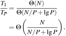
When lgP is insignificant compared to N, the asymptotic speedup is Θ(P). The asymptotic efficiency is:
![]() (2.13)
(2.13)
When ![]() , the asymptotic efficiency is
, the asymptotic efficiency is ![]() . Note that extra lgP factor. Merely scaling up the input by a factor of P is not enough to deliver
. Note that extra lgP factor. Merely scaling up the input by a factor of P is not enough to deliver ![]() weak scaling as P grows.
weak scaling as P grows.
Remember that if there is a better serial algorithm that does not parallelize well, it is fairer to use that algorithm for T1 when comparing algorithms. Do not despair if a parallelized algorithm does not get near 100% parallel efficiency, however. Few algorithms do. Indeed, an efficiency of ![]() is “break even” in a sense. At the turn of the century, speed improvements from adding transistors were diminishing, to the point where serial computer speed was growing as the square root of the number of transistors on a chip. So if the transistors for P workers were all devoted to making a single super-worker faster, that super-worker would speed up by about
is “break even” in a sense. At the turn of the century, speed improvements from adding transistors were diminishing, to the point where serial computer speed was growing as the square root of the number of transistors on a chip. So if the transistors for P workers were all devoted to making a single super-worker faster, that super-worker would speed up by about ![]() . That’s an efficiency of only
. That’s an efficiency of only ![]() . So if your efficiency is significantly better than
. So if your efficiency is significantly better than ![]() , your algorithm really is still benefitting from the parallel revolution.
, your algorithm really is still benefitting from the parallel revolution.
2.5.9 Little’s Formula
Little’s formula relates the throughput and latency of a system to its concurrency. Consider a system in steady state that has items to be processed arriving at regular intervals, where the desired throughput rate is R items per unit time, the latency to process each item is L units of time, and the number of items concurrently in the system is C. Little’s formula states the following relation between these three quantities:
![]() (2.14)
(2.14)
Concurrency is similar but not identical to parallelism. In parallelism, all work is going on at the same time. Concurrency is the total number of tasks that are in progress at the same time, although they may not all be running simultaneously. Concurrency is a more general term that includes actual parallelism but also simulated parallelism, for example by time-slicing on a scalar processor.
Extra concurrency can be used to improve throughput when there are long latency operations in each task. For example, memory reads that miss in cache can take a long time to complete, relative to the speed at which the processor can execute instructions. While the processor is waiting for such long-latency operations to complete, if there is other work to do, it can switch to other tasks instead of just waiting. The same concept can be used to hide the latency of disk transactions, but since the latency is so much higher for disk transactions correspondingly more parallelism is needed to hide it.
Suppose a core executes 1 operation per clock, and each operation waits on one memory access with a latency L of 3 clocks. The latency is fully hidden when there are ![]() operations in flight. To be in flight simultaneously, those operations need to be independent. Hardware often tries to detect such opportunities in a single thread, but often there are not enough to reach the desired concurrency C. Hardware multithreading can be used to increase the number of operations in flight, if the programmer specifies sufficient parallelism to keep the hardware threads busy. Most famously, the Tera MTA had 128 threads per processor, and each thread could have up to 8 memory references in flight [SCB+98]. That allowed it to hide memory latency so well that its designers eliminated caches altogether!
operations in flight. To be in flight simultaneously, those operations need to be independent. Hardware often tries to detect such opportunities in a single thread, but often there are not enough to reach the desired concurrency C. Hardware multithreading can be used to increase the number of operations in flight, if the programmer specifies sufficient parallelism to keep the hardware threads busy. Most famously, the Tera MTA had 128 threads per processor, and each thread could have up to 8 memory references in flight [SCB+98]. That allowed it to hide memory latency so well that its designers eliminated caches altogether!
The bottom line is that parallelizing to hide latency and maximize throughput requires over-decomposing a problem to generate extra concurrency per physical unit.
Be warned, however, that hardware multithreading can worsen latency in some cases. The problem is that the multiple threads typically share a fixed-size cache. If n of these threads access disjoint sets of memory locations, each gets a fraction 1/n of the cache. If the concurrency is insufficient to fully hide the latency of the additional cache misses, running a single thread might be faster.
2.6 Pitfalls
Parallel programming entails additional pitfalls any time there are dependencies between parallel tasks. Dependencies between parallel tasks require synchronization. Too little synchronization can lead to non-deterministic behavior. Too much synchronization can unnecessarily limit scaling, or worse yet, cause deadlock.
2.6.1 Race Conditions
A race condition occurs when concurrent tasks perform operations on the same memory location without proper synchronization, and one of the memory operations is a write. Code with a race may operate correctly sometimes but fail unpredictably at other times. Consider the code in Table 2.2, where two tasks attempt to add 1 and 2 respectively to a shared variable X. The intended net effect is likely to be X += 3. But because of the lack of synchronization, two other net effects are possible: X += 1 or X += 2. To see how one of the updates could be lost, consider what happens if both tasks read X before either one writes to it. When the writes to X occur, the effect of the first write will be lost when the second write happens. Eliminating temporary variables and writing X += 1 and Y += 1 does not help, because the compiler might generate multiple instructions anyway, or the hardware might even break += into multiple operations.
Table 2.2. Two tasks race to update shared variable X. Interleaving can cause one of the updates to be lost.
| Task A | Task B |
| a = X; | b = X; |
| a += 1; | b += 2; |
| X = a; | X = b; |
Race conditions are pernicious because they do not necessarily produce obvious failures and yet can lead to corrupted data [Adv10, Boe11]. If you are unlucky, a program with a race can work fine during testing but fail once it is in the customer’s hands. Races are not limited to memory locations. They can happen with files and I/O too. For example, if two tasks try to print Hello at the same time, the output might look like HeHelllloo.
Surprisingly, analyzing all possible interleaving of instructions is not enough to predict the outcome of a race, because different hardware threads may see the same events occur in different orders. The cause is not relativistic physics, but the memory system. However, the effects can be equally counterintuitive. Table 2.3 shows one such example. It is representative of the key part of certain synchronization algorithms. Assume that X and Y are initially zero. After tasks A and B execute the code, what are the possible values for a and b? A naive approach is to assume sequential consistency, which means that the instructions behave as if they were interleaved in some serial order. Figure 2.10 summarizes the possible interleavings. The first two graphs show two possible interleavings. The last graph shows a partial ordering that accounts for four interleavings. Below each graph is the final outcome for a and b.
Table 2.3. Race not explainable by serial interleaving. Assume that X and Y are initially zero. After both tasks complete, both a and b can be zero, even though such an outcome is impossible by serial interleaving of the instruction streams.
| Task A | Task B |
| X = 1; | Y = 1; |
| a = Y; | b = X; |
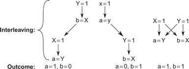
Figure 2.10 All sequentially consistent outcomes of Table 2.3. The graphs summarize all possible interleavings of instructions from Table 2.3, yet real hardware can deliver the outcome a = 0 and b = 0.
Yet when run on modern hardware, the set of all possible outcomes can also include a = 0 and b = 0! Modern hardware is often not sequentially consistent. For example, the compiler or hardware may reorder the operations so that Task A sees Task B read Y before it writes X. Task B may see Task A similarly reordered. Each task sees that it executed instructions in the correct order and sees the other task deviate. Table 2.4 shows what the two tasks might see. Both are correct, because there is no global ordering of operations to different memory locations. There are system-specific ways to stop the compiler or hardware from reordering operations, called memory fences [AMSS10, Cor11a, TvPG06], but these are beyond the scope of this book. Instead, we will emphasize machine-independent techniques to avoid races altogether.
Table 2.4. No global ordering of operations to different locations. The hardware might reorder the operations from Table 2.3 so that different tasks see the operations happen in different orders. In each view, a task sees its own operations in the order specified by the original program.
| Viewpoint of Task B | Viewpoint of Task A |
| a = Y | b = X |
| b = X | a = Y |
| Y = 1 | X = 1 |
| X = 1 | Y = 1 |
The discussion here should impress upon you that races are tricky. Fortunately, the patterns in this book, as well as the programming models we will discuss, let you avoid races and not have to think about tricky memory ordering issues. This is a good thing because memory ordering is exactly the kind of thing that is likely to change with future hardware. Depending too much on the low-level implementation of current memory systems will likely lead to code that will be difficult to port to future processors.
2.6.2 Mutual Exclusion and Locks
Locks are a low-level way to eliminate races. This section explains what locks are and why they should be a means of last resort. Perhaps surprisingly, none of the examples in the rest of this book requires a lock. However, sometimes locks are the best way to synchronize part of a program.
The race in Table 2.2 can be eliminated by a mutual exclusion region. Using mutual exclusion, the tasks can coordinate so they take turns updating X, rather than both trying to do it at once. Mutual exclusion is typically implemented with a lock, often called a mutex. A mutex has two states, locked and unlocked, and two operations:
These operations are implemented atomically, meaning that they appear instantaneous to other tasks and are sequentially consistent.
The lock operation on an already locked mutex must wait until it becomes unlocked. Once a task completes a lock operation, it is said to own the mutex or hold a lock until it unlocks it. Table 2.5 shows how to use a mutex to remove the race in Table 2.2. Mutex M is presumed to be declared where X is declared. The lock–unlock operations around the updates of X ensure that the threads take their turn updating it. Furthermore, the lock–unlock pair of operations demarcate a “cage.” Instruction reordering is prohibited from allowing instructions inside the cage to appear to execute outside the cage, preventing counterintuitive surprises. However, be aware that other threads might see instructions written outside the cage appear to execute inside the cage.
Table 2.5. Mutex eliminates the race in Table 2.2. The mutex M serializes updates of X, so neither update corrupts the other one.
| Task A | Task B |
| extern tbb::mutex M; | extern tbb::mutex M; |
| M.lock(); | M.lock(); |
| a = X; | b = X; |
| a += 1; | b += 2; |
| X = a; | X = b; |
| M.unlock(); | M.unlock(); |
An important point about mutexes is that they should be used to protect logical invariants, not memory locations. In our example, the invariant is “the value of X is the sum of the values added to it.” What this means is that the invariant is true outside the mutual exclusion region, but within the region we may have a sequence of operations that might temporarily violate it. However, the mutex groups these operations together so they can be treated essentially as a single operation that does not violate the invariant. Just using a mutex around each individual read or write would protect the memory location, but not the invariant. In particular, such an arrangement might expose temporary states in which the invariant is violated. In more complex examples, such as with data structures, a mutex protects an invariant among multiple locations. For example, a mutex protecting a linked list might protect the invariant “the next field of each element points to the next element in the list.” In such a scheme, any time a task traverses the list, it must first lock the mutex; otherwise, it might walk next fields under construction by another task.
2.6.3 Deadlock
Deadlock occurs when at least two tasks wait for each other and each cannot resume until the other task proceeds. This happens easily when code requires locking of multiple mutexes at once. If Task A needs to lock mutexes M and N, it might lock M first and then try to lock N. Meanwhile, if Task B needs the same two locks but locks N first and then tries to lock M, both A and B will wait forever if the timing is such that each performs the first locking operation before attempting the second. This situation is called deadlock. The impasse can be resolved only if one task releases the lock it is holding.
There are several ways to avoid deadlock arising from mutexes:
Avoid mutexes when possible. Consider replicating the resource protected by the mutex. Alternatively, synchronize access to it using a higher-level pattern. For example, Section 12.2 shows how to use tbb::pipeline to serialize access to input and output files without any mutexes. In Intel Cilk Plus, hyperobjects (see Section 8.10) often eliminate the need for explicit mutual exclusion by way of implicit replication. The Intel ArBB programming model uses deterministic data-parallel patterns and manages without locks at all. In some cases, the TBB concurrent collections, which are based on atomic operations rather than locks, can be used for shared data structures.
Hold at most one lock at a time. An important corollary of this rule is never call other people’s code while holding a lock unless you are certain that the other code never acquires a lock.
Always acquire locks on multiple mutexes in the same order. In the earlier example, deadlock is avoided if Task A and Task B both always try to lock mutex X first before trying to lock mutex Y.
Some common tactics for achieving the “same order” strategy include:
Stratify the mutexes. Assign each mutex a level such that two mutexes on the same level are never locked at the same time, then always acquire locks in level order. For example, in a tree where there is a mutex for each tree node, the levels might correspond to levels in a tree.
Sort the mutexes to be locked. If you always know the entire set of locks to be acquired before acquiring any of them, sort the mutex addresses and acquire the locks in that order. Note: if the memory allocations are not the same from run to run of the program, which might be accidental (non-deterministic memory allocation) or intentional (randomization of memory allocations for increased security), then the order may be different on different runs, complicating debugging and profiling.
Backoff. When acquiring a set of locks, if any lock cannot be acquired immediately, release all locks already acquired. This approach requires that the mutex support a “try lock” operation that immediately returns if the lock cannot be acquired.
Locks are not intrinsically evil. Sometimes they are the best solution to a synchronization problem. Indeed, TBB provides several kinds of mutexes for use with it and other programming models. But consider the alternatives to locks and avoid them if you can. If you must use locks, be careful to avoid situations that can cause deadlock.
Locks are not the only way to stumble into deadlock. Any time you write code that involves “wait until something happens,” you need to ensure that “something” is not dependent on the current task doing anything else.
2.6.4 Strangled Scaling
Deadlock is not the only potential problem arising from synchronization. By definition, a mutex serializes execution and adds a potential Amdahl bottleneck. When tasks contend for the same mutex, the impact on scaling can be severe, even worse than if the protected code was serial. Not only does Amdahl bottleneck come into play, but the status of the protected memory locations must be communicated between cores, thus adding communication costs not paid by the serial equivalent.
Sometimes when profiling a piece of parallel code, the profiler reports that most of the time is spent in a lock operation. A common mistake is to blame the implementation of the mutex and say “if only I had a faster mutex.” The real problem is using the mutex at all. It is just doing its job—serializing execution.
A mutex is only a potential bottleneck. If tasks rarely contend for the same mutex, the impact of the mutex on scaling is minor. Indeed, the technique of fine-grain locking replaces a single highly contended lock with many uncontended locks, and this can improve scalability by reducing contention. For example, each row of a matrix might be protected by a separate mutex, rather than a single lock for the entire matrix, if there are no invariants across different rows. As long as tasks rarely contend for the same row, the impact on scaling should be beneficial. Fine grain locking is tricky, however, and we do not discuss it further in this book. It is sometimes used inside the implementation of Intel Cilk Plus and Intel TBB, but you do not have to know that. The point is that mutexes can limit scalability if misused. The high-level patterns in the rest of this book let you avoid mutexes in most cases.
As a final note, you can sometimes use atomic operations in place of mutexes if the logical invariant involves a single memory location, and much of the synchronization constructs inside Intel Cilk Plus and Intel TBB are built with atomic operations. Atomic operations are discussed briefly in Section C.10.
2.6.5 Lack of Locality
Locality is the other key to scaling. Remember that work, span, and communication are the three key concerns. Locality refers to two bets on future memory accesses after a core accesses a location:
Temporal locality: The core is likely to access the same location again in the near future.
Spatial locality: The core is likely to access nearby locations in the near future.
Having good locality in a program means the hardware can win its bets since the above statements are more likely to be true. Hardware based on these assumptions being true can reduce communication. For example, as noted in Section 2.4.1, a memory access pulls an entire cache line (a small block of memory) around that memory location onto the chip and into the cache. Using the data on that line repeatedly while the cache line is resident is faster than pulling it in multiple times. To take advantage of this, programs should be written so they process data thoroughly and completely before moving to process other data. This increases the number of times the data will be found in cache, and will avoid reading the same data multiple times from off-chip memory. Cache oblivious algorithms [ABF05] (Section 8.8) are a formal way of exploiting this principle. Such algorithms are designed to have good locality at multiple scales, so it does not matter what specific size the cache line is.
Communication is so expensive and computation so cheap that sometimes it pays to increase the work in exchange for reducing communication. On current hardware, a cache miss can take up to the order of a hundred cycles. So it often pays to duplicate trivial calculations rather than try to do them in one place and share, and there is nascent research into communication avoiding algorithms [GDX08].
2.6.6 Load Imbalance
A load imbalance is the uneven distribution of work across workers. Figure 2.11 shows how load imbalance can impact scalability. In this figure, the parallel work was broken up into tasks, with one task per worker. The time taken by the longest-running task contributes to the span, which limits how fast the parallelized portion can run.
Figure 2.11 Load imbalance. Variation in the execution time of parallel tasks can reduce scalability.
Load imbalance can be mitigated by over-decomposition, dividing the work into more tasks than there are workers. Like packing suitcases, it is easier to spread out many small items evenly than a few big items. This is shown in Figure 2.12. Some processors have fewer tasks than others. There is still a possibility that a very long task will get scheduled at the end of a run, but the parallel slack nonetheless improves the predictability of parallel execution times.
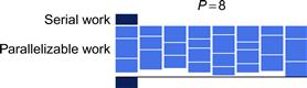
Figure 2.12 Overdecomposition can improve load balancing. Subdividing the parallel work into more tasks than workers permits the scheduler to pack tasks onto workers and improve load balance.
2.6.7 Overhead
Parallelization introduces additional overhead to launch and synchronize tasks, as shown in Figure 2.13. This overhead increases both work and span. The additional tasks incurred by overdecomposition tends to increase this overhead, since there is usually a fixed amount of overhead for managing every task. Making tasks too small can increase execution time and can also decrease arithmetic intensity. Therefore, there is a tension between providing sufficient overdecomposition to allow for balancing the load while still making tasks large enough to amortize synchronization overhead and maximize arithmetic intensity.
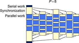
Figure 2.13 Overhead can reduce scalability. Distributing tasks to workers, starting tasks, and synchronizing completion adds to execution time. Tree-based schemes can reduce, but not eliminate, this overhead.
Careful synchronization design can reduce overhead, but cannot completely eliminate it. In the example in Figure 2.13, the overhead for launching and synchronizing a large number of independent tasks can use a tree structure, so that startup is logarithmic in the number of workers, instead of linear as would occur if all parallel tasks were launched from one task. This makes the launching and synchronization time logarithmic in the number of workers rather than linear, but it nonetheless grows with the number of workers.
2.7 Summary
This chapter covered a lot of theoretical and practical background. Although we do not want to dwell on computer architecture in this book, we have presented a simple summary of current trends in computer architecture as a basis for later discussion.
We also discussed many factors related to performance and presented some key definitions, including those of latency and throughput. Amdahl’s Law and Gustafson’s Law were presented and give bounds on performance, but we highly recommend the use of the work-span model for more accuracy. The work-span model not only accounts for imperfect parallelization but also gives a lower bound as well as an upper bound on speedup.
We also discussed several pitfalls that can lead to problems in parallel programs, from poor scalability to incorrect behavior. Race conditions and deadlock can be avoided with careful design. Assuming you achieve a correct program, of course you then want it to scale in performance. Scalability can be difficult to achieve, but here are some key rules of thumb:
• Make the available parallelism scale with the data.
• Keep the span short; avoid adding extra work for parallelism.
• Over-decompose to provide parallel slack.
• Minimize synchronization. Avoid locks.
• Use locality to minimize memory traffic. Be aware that the quantum of memory traffic is a cache line.
The rest of this book is about structured ways to achieve these goals.