
Wing Design
Abstract
Wing design is addressed utilizing standard methods for preliminary comparative aerodynamics and stability and control evaluations. General wing planform characteristics are discussed. Airfoil characteristics and performance including compressibility effects are covered including wing maximum lift in the cruise configuration and effects of Reynolds number in flight. Design methods for swept and twisted wings with varying airfoil sections are handled by several methods. Maximum wing lift is calculated using both modified lifting line theory and the pressure difference rule. High lift devices including trailing-edge flaps, leading-edge slats or flaps, and methods for determination of maximum lift in the takeoff and landing configurations are considered. Development and layout of the preliminary wing design, including aspect ratio, taper ratio, wing relative thickness, and airfoil selection are described. Effects of wing-mounted and fuselage-mounted engines, placement of high lift devices, use of winglets and raked wingtips, and wing dihedral and incidence are discussed.
Keywords
Airfoils
Supercritical airfoil
Swept wings
High lift devices
Lifting line
Lifting surface methods
5.1 General wing planform characteristics
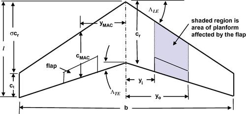
A general wing planform shape is shown in Figure 5.1. In this case an ogee shape somewhat like that of the Concorde supersonic airliner is depicted. The main parameters of importance are shown in the figure. The overall length of the wing l and the wingspan b are readily apparent and the centroid of the wing area is indicated. The x-axis is an axis of symmetry and the chord length is defined as the distance between the leading and trailing edges of the wing as measured parallel to the centerline of symmetry, that is, the x-axis. Thus the chord length is a function of spanwise distance y and is denoted by c(y) with the root chord being measured along the centerline, y = 0, and is denoted by cr = c(0).
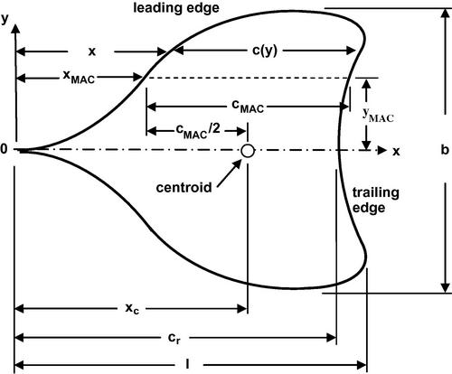
The wing area S is defined as the planform area, that is, the projected area on the x-y plane, and it is commonly taken as the reference area for most airplane performance calculations. Part of the wing planform may be obstructed by the fuselage and to complete the full planform the leading and trailing edges are faired in to the centerline in a consistent and reasonable fashion. The area is then given by
The mean aerodynamic chord cMAC is defined as
The centroid of the wing planform area lies on the centerline of symmetry and its location xc on that line may be found from the equation for the moment of the area about the origin:
Here the xLE is the distance from the y-axis to the leading edge of the chord. Solving for the centroid location yields
Note that the centroid location may also be expressed as the sum of the distance from the origin to the leading edge point of the mean aerodynamic chord and the mean aerodynamic chord length as follows:
![]()
Here xMAC is the distance from the origin to the leading edge point of the mean aerodynamic chord. The spanwise location of the mean aerodynamic chord is denoted yMAC. Another important parameter is the aspect ratio of the wing which is defined as

The slenderness of the wing is suggested by the aspect ratio, as may be seen by considering the wing to have an average chord length cavg such that S = bcavg. Then the aspect ratio A = b/cavg and a large aspect ratio would represent a wingspan much greater than the average chord length. Similarly one may consider the aspect ratio to be the ratio of the area of a square formed by the wingspan, that is, b2, to the actual planform area S. Another characteristic of the slenderness of a wing is the ratio b/l, where l is the overall length of the wing measured from the apex of the wing to its most aft point.
5.1.1 The straight-tapered wing planform
A conventional wing planform is characterized by straight leading and trailing edges as shown in Figure 5.2. The general wing parameters may be readily calculated for this type of wing.
The defining features of the straight-tapered wing are the sweepback angles of the leading and trailing edge, ΛLE and ΛTE, respectively, and the taper ratio λ = ct/cr. The wing planform area defined by Equation (5.1) may be written as
The mean aerodynamic chord defined by Equation (1.2) becomes
The centroid location defined by Equation (5.3) is
The quantity σ, depicted in Figure 5.2, is defined as follows:

The aspect ratio, Equation (5.4), becomes
The spanwise location of the mean aerodynamic chord is
The sweepback of different chordwise locations is often needed in the design process, particularly the quarter-chord and half-chord positions. The sweepback of any location n, as a fraction of the chord, may be found from the known sweepback at some other position m, also as a fraction of chord, as follows:
For example, if the leading edge sweepback angle is ΛLE = Λ0, then the quarter-chord sweepback angle Λc/4 = Λ0.25 and

Assuming typical values ΛLE = 30°, A = 9, and λ = 1/3 we find that Λc/4 = 27.56°.
5.1.2 Cranked wing planform
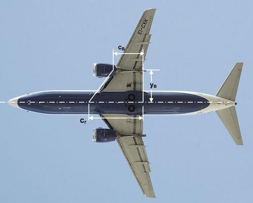
It is sometimes advantageous to employ a cranked wing planform, that is, one with discontinuous changes in sweepback angle of the leading and/or trailing edges, like that shown in Figure 5.3. Some commercial airliners have essentially zero sweepback along the trailing edge in the central portion of the wing as shown in Figure 5.4. This design feature, sometimes called a “yehudi,” allows for better stowage of landing gear, cargo, and a stronger wing root structure. In addition to these intuitively obvious attributes, the longer chord length in the vicinity of the fuselage junction provides for improved aerodynamic flow characteristics over the wing.
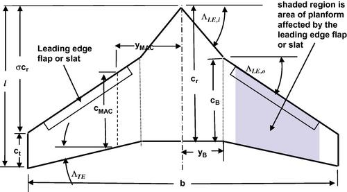
For the case of a single kink at one spanwise location on the leading and/or trailing edge, as shown in Figure 5.3 or 5.4 we may readily find the important geometrical properties of the wing. The area may be considered to be comprised of the sum of the inner panel area Si and outer panel area So, or
This may be put in the form
Here we have introduced yB, the spanwise distance outboard to the break in trailing edge angle, and λi = cB/cr, the taper ratio of the inboard panel. The aspect ratio is
The mean aerodynamic chord may be written in terms of the mean aerodynamic chord of the inner and outer panels as follows:
![]()
The mean aerodynamic chord then may be written as
The spanwise location of the mean aerodynamic chord may be written in terms of the spanwise location of the mean aerodynamic chord in each panel:
![]()
Similarly the spanwise location of the mean aerodynamic chord is given by
The wing area centroid is given by
The location of the leading edge of the mean aerodynamic chord is given in terms of the spanwise location of the mean aerodynamic chord in the inner and outer panels as follows:
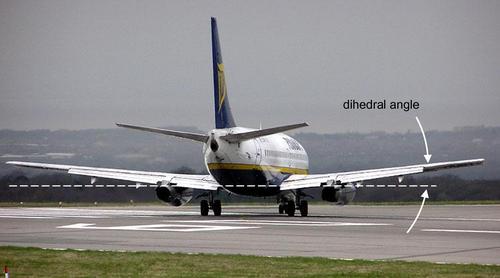
5.1.3 Wing dihedral
The planform views discussed thus far cannot illustrate another common wing characteristic, dihedral. This is the angle that a wing makes with a horizontal line like the ground plane as illustrated in Figure 5.5. It is typically a small angle, on the order of 3–8°. This angle has an influence on the stability of an aircraft in roll and will be the subject of discussion in a later chapter.
5.2 General airfoil characteristics
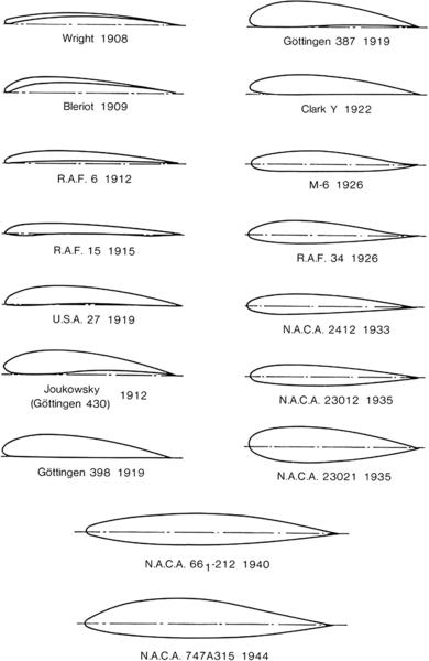
A cross-section taken through the wing planform in Figure 5.3 at a general spanwise location y = constant reveals a shape called the airfoil section. The historical evolution of airfoil sections, over the period 1908 through 1944, is illustrated in Figure 5.6. The last two shapes shown (NACA 661-212 and NACA 747A315) are considered low-drag sections. The NACA 6-series airfoils were designed to maintain laminar flow over 60–70% of chord on both the upper and the lower surface. The objective was to reduce drag and increase the critical Mach number, that is, the speed at which compressibility effects become important. The NACA 7-series airfoils were designed to have a greater extent of laminar flow on the lower surface than on the upper surface. This was aimed at producing lower pitching moments at the expense of some reduction in critical Mach number. Note that these later laminar flow airfoils are thickest near the center of their chords. Among the classical airfoil sections, those of the NACA 6-series laminar flow airfoils are most appropriate for the design project because they have the best high-speed characteristics.
A full discussion of the systematic development of NACA airfoils, along with tabular listings of their coordinates and graphical presentation of their aerodynamic characteristics, is given in the book by Abbott and Von Doenhoff (1959) which is based on earlier work by Abbott et al. (1945). A computer program for generating the shapes of the NACA airfoils is presented by Ladson et al. (1996).
5.2.1 Airfoil sections
The NACA families airfoils are obtained by combining a mean line and a thickness distribution as illustrated in Figure 5.7. In the NACA 6-series of airfoils the mean camber lines (the locus of the centers of circles tangent to the upper and lower surfaces) are designed to have uniform chordwise pressure loading, Δp = pl − pu, up to a particular chordwise station x/c = a and then to linearly decrease to zero at the trailing edge. The thickness distribution is designed to fix the chordwise (x/c) location of the minimum pressure for the symmetric form of the airfoil (straight camber line, y = 0) at the point of maximum thickness (t/c)max.
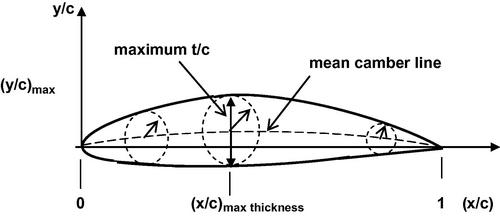
Figure 5.7 Airfoil showing the mean camber line, the maximum thickness to chord ratio and, its position along the chord.
The numbering system for the NACA 6-series may be explained using an example, say the NACA 653-218, a = 0.5 airfoil. In this case
6: denotes the NACA 6-series of sections
5: denotes the chordwise position of the minimum value of pressure coefficient (Cp,min), measured in tenths of chord, for the basic symmetric thickness section at zero lift
3: denotes the range of lift coefficients, in tenths, above and below the design lift coefficient cL,des, for which a favorable pressure gradient exists on both the upper and lower surfaces and drag coefficient is lowest
2: denotes the design lift coefficient multiplied by 10; here cl,des = 0.2
18: denotes the thickness in percent chord, here 18%; for values below 10% the thickness ratio would be entered with a prefix 0, as, for example, 08 for 8%
a: denotes the type of mean line used, in this case the mean line has a uniform load up to x/c = a = 0.5. When no mean line designation is given it is understood that the uniform load mean line (a = 1) has been used
Modifications to the basic airfoil numbering system sometime arise as a result of alterations to a basic airfoil shape. The most common is the replacement of the dash by a capital letter, such as in the NACA 641A212. The letter A denotes a change in the shape of the aft portion of the airfoil where the upper and lower surfaces remain essentially straight from about x/c = 0.8 to the trailing edge. This modification was introduced to simplify manufacturing as well as to avoid a wing with a thin and sharp trailing edge which is prone to stress concentration and buckling. For explanations of other, less common, variations in the airfoil designations see Abbott and Von Doenhoff (1959).
Loftin (1948) points out that NACA 6-series airfoil sections with small thickness to chord ratios have relatively high critical Mach numbers but have the disadvantage of being impractically thin near the trailing edge so that substantial fabrication difficulties are encountered. To alleviate this problem the cusped trailing edge has been eliminated from a number of NACA 6-series basic thickness forms and replaced by essentially straight segments from approximately 80% chord to the trailing edge so as to form a finite trailing edge angle. These new sections have been designated the NACA 6A-series airfoil sections as previously indicated. Experimental results obtained at Reynolds numbers of 3–9 million based on chord length indicate that the section minimum drag and maximum lift characteristics of comparable NACA 6-series and 6A-series airfoil sections are essentially the same. The quarter-chord pitching-moment coefficients and angles of zero lift of NACA 6A-series airfoil sections are slightly more negative than those of corresponding NACA 6-series airfoil sections. The position of the aerodynamic center and the lift curve slope of smooth NACA 6A-series airfoil sections appear to be essentially independent of airfoil thickness ratio in contrast to the trends shown by NACA 6-series sections.
There was a resurgence of airfoil development in the 1960s and 1970s following a long hiatus in the two decades following the Second World War. NASA launched a concerted effort to develop new airfoil sections that would have improved performance at high subsonic Mach numbers and thereby improve the performance of the newly introduced turbojet airliners. In particular, designs were sought that would delay the drag divergence Mach number and maintain reasonable drag coefficients at the turbulent flow conditions typical of high-speed flight while retaining acceptable maximum lift and stall characteristics at the low speeds typical of landing. This research led to the so-called supercritical airfoil, one that has a distinctive shape compared to standard airfoils. A description of these developments is given by Harris (1990).
Airframe manufacturers have been actively engaged in this work, but their results are proprietary, and generally not publicly released. Several of the NASA supercritical airfoils are described by Harris (1990) and relevant NASA publications cited therein are generally available online through the NASA Technical Report Server. McCormick (1995) also discusses some supercritical airfoils. There is as yet no other single source which collects and summarizes a wide range of supercritical airfoil theories and results as do Abbott and Von Doenhoff (1959) for conventional airfoils. For these reasons, and for those of expediency and completeness of information supplied, it is suggested that NACA airfoils be used for the preliminary design. The use of advanced CFD codes for airplane design in industry, as described, for example, by Jameson (1989), has led to integrated design of complete three-dimensional wings, bypassing the approach presented in this book, which uses two-dimensional airfoil characteristics to fashion a three-dimensional wing. However, the latter approach is important in developing an understanding of the contribution of the different elements of a wing to its overall performance. Therefore in the preliminary design phase it is considered practical, efficient, and educationally sound to use this building block approach.
5.2.2 Airfoils at angle of attack
A great deal of theoretical and experimental work has been devoted to the development of airfoil sections. Theoretical airfoil design is hampered by the existence of viscous effects in the form of a “boundary layer” of low-energy air between the airfoil surface and the outer flow within which friction is important and outside of which friction is negligible. The viscous boundary layer has major effects on airfoil drag and maximum lift characteristics but only relatively minor effects on lift curve slope, angle of attack for zero lift, and section pitching-moment coefficient.
Because the boundary layer itself is influenced by surface roughness, surface curvature, pressure gradient, heat transfer between the surface and the boundary layer, and viscous interaction with the free stream it is apparent that no simple theoretical considerations can accurately predict all the airfoil characteristics. For these reasons, experimental data are always preferable to theoretical calculations. Airfoils have been optimized for many specific characteristics, including: high maximum lift, low drag at low lift coefficients, low drag at high lift coefficients, low pitching moments, low drag in the transonic region, and favorable lift characteristics beyond the critical Mach number. Optimization of an airfoil in one direction usually compromises it in another. Thus, low-drag airfoil designs often are prone to exhibiting poor high lift characteristics while high lift airfoil designs tend to show low critical Mach numbers.
Graphical representations of the experimental data gathered for many NACA airfoils by Abbott and Von Doenhoff (1959) are represented in Appendix A for selected airfoils. The data are mainly for smooth surface conditions and are shown for Reynolds numbers from 3 × 10⁶ to 9 × 10⁶ based on chord length. However, some data at a Reynolds number of 6 × 10⁶ are also shown for airfoils where fine grit has been lightly deposited on the surface of the leading edge region for distances up to about 8% of the chord length in order to initiate turbulence in the boundary layer. These cases are denoted by the term “standard roughness.” From these data the following airfoil characteristics for smooth surfaces have been collected:
1. Angle of attack at zero lift, α0.
2. Moment coefficient at the quarter-chord point at zero lift, cm,0.
3. Lift curve slope, cl,α.
4. Aerodynamic center location in percent chord, a.c.
5. Angle of attack for maximum lift coefficient, ![]() .
.
6. Maximum lift coefficient, ![]() .
.
7. Angle of attack at which the lift curve deviates from linear variation, α0.
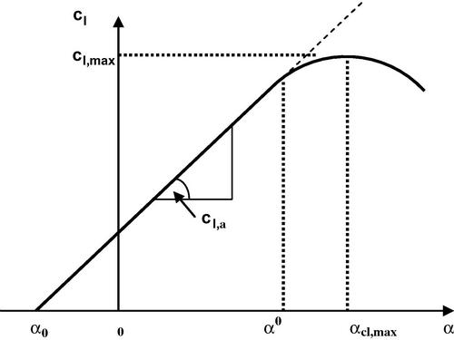
Results for a number of smooth NACA 6-series airfoils at a Reynolds number Rec = 9 × 10⁶ are presented in Table 5.1. From items 1, 3, 5, 6, and 7 an approximate section lift curve shape can be synthesized, as illustrated in Figure 5.8. It is apparent from the above that any generalized charts for airfoil section characteristics, including the ones in this book, must be used with caution. Tabulated experimental and theoretical data for other NACA airfoils are presented in Hoak et al. (1978).
Basic Characteristics of Selected NACA Airfoils at a Reynolds number Rec = 9 × 10⁶
| Airfoil | α0 (deg) | cm,0 | clα | a.c. | αcl,max | cl,max | α0w |
| 63-006 | 0 | 0.005 | 0.112 | 0.258 | 10.0 | 0.87 | 7.7 |
| 63-009 | 0 | 0 | 0.111 | 0.258 | 11.0 | 1.15 | 10.7 |
| 631-012 | 0 | 0 | 0.116 | 0.265 | 14.0 | 1.45 | 12.3 |
| 632-015 | 0 | 0 | 0.117 | 0.271 | 14.5 | 1.47 | 11.0 |
| 633-018 | 0 | 0 | 0.115 | 0.271 | 15.5 | 1.54 | 11.2 |
| 634-021 | 0 | 0 | 0.118 | 0.273 | 17.0 | 1.38 | 9.0 |
| 63-206 | −1.9 | −0.037 | 0.112 | 0.254 | 10.5 | 1.06 | 6.0 |
| 63-209 | −1.4 | −0.032 | 0.11 | 0.262 | 12.0 | 1.4 | 10.3 |
| 63-210 | −1.2 | −0.035 | 0.113 | 0.261 | 14.5 | 1.56 | 9.6 |
| 631-212 | −2.0 | −0.035 | 0.114 | 0.263 | 14.5 | 1.63 | 11.4 |
| 632-215 | −1.0 | −0.03 | 0.116 | 0.267 | 15.0 | 1.60 | 8.8 |
| 633-218 | −1.4 | −0.033 | 0.118 | 0.271 | 14.5 | 1.85 | 8.0 |
| 634-221 | −1.5 | −0.035 | 0.118 | 0.269 | 15.0 | 1.44 | 9.2 |
| 634-421 | −2.2 | −0.056 | 0.109 | 0.265 | 14.0 | 1.42 | 7.6 |
| 64-206 | −1.0 | −0.040 | 0.110 | 0.253 | 12.0 | 1.03 | 8.0 |
| 64-208 | −1.2 | −0.039 | 0.113 | 0.257 | 10.5 | 1.23 | 8.8 |
| 64-209 | −1.5 | −0.040 | 0.107 | 0.261 | 13.0 | 1.40 | 8.9 |
| 64-210 | −1.6 | −0.040 | 0.110 | 0.253 | 14.0 | 1.45 | 10.8 |
| 641-212 | −1.3 | −0.027 | 0.113 | 0.262 | 15.0 | 1.55 | 11.0 |
| 642-215 | −1.6 | −0.030 | 0.112 | 0.265 | 15.0 | 1.57 | 10.0 |
| 643-218 | −1.3 | −0.027 | 0.115 | 0.271 | 16.0 | 1.53 | 10.0 |
| 644-221 | −1.2 | −0.029 | 0.117 | 0.271 | 13.0 | 1.32 | 6.8 |
| 641-412 | −2.6 | −0.065 | 0.112 | 0.267 | 15.0 | 1.67 | 8.0 |
| 642-415 | −2.8 | −0.070 | 0.115 | 0.264 | 15.0 | 1.65 | 8.0 |
| 643-418 | −2.9 | −0.065 | 0.116 | 0.273 | 14.0 | 1.57 | 8.0 |
| 644-421 | −2.8 | −0.068 | 0.120 | 0.276 | 13.0 | 1.42 | 6.4 |
| 63A010 | 0 | 0.005 | 0.105 | 0.254 | 13.0 | 1.20 | 10.0 |
| 63A210 | −1.5 | −0.040 | 0.103 | 0.254 | 14.0 | 1.23 | 10.0 |
| 64A010 | 0 | 0 | 0.110 | 0.253 | 12.0 | 1.23 | 10.0 |
| 64A210 | −1.5 | −0.040 | 0.105 | 0.251 | 8.0 | 1.44 | 10.0 |

The systematic compilation of aerodynamic data for various families of NACA airfoils presented by Abbott et al. (1945) and mentioned above covered a range of Reynolds numbers suitable for the aircraft of that period. However, soon afterwards, the development of larger and faster aircraft exposed the need for airfoil data at still higher Reynolds numbers. In response to this need Loftin and Bursnall (1948) carried out experiments on selected NACA airfoils at Reynolds numbers up to 25 × 106. The main conclusion of that research was that the airfoil lift curve slope was essentially unaffected by the increase in Reynolds number, remaining remarkably close to the theoretical value a = 2π per radian or a = 0.11 per degree. On the other hand, the airfoil maximum lift coefficient cl,max for the relatively thin airfoils tested (t/c ≤ 12%) showed a constant value for Rec up to about 6 × 10⁶, then a small increase of up to 10% as Rec approached 15 × 106, and finally a constant or slightly falling value up to Rec = 25 × 106, the maximum value tested. Relatively thick airfoils (t/c > 18%) displayed different behavior with a slow but monotonic increase in cl,max up to the maximum Reynolds numbers tested. The effect of roughness was found to be minimal for both lift curve slope and maximum lift coefficient throughout the range of Reynolds number tested. The roughness is assumed to trip the boundary layer so that it is completely turbulent over the entire Reynolds number range and therefore is no longer sensitive to Reynolds number. Abbott and Von Doenhoff (1959) discuss the effects of Reynolds number for all the NACA airfoils originally presented by Abbott et al. (1945) in some detail, but only up to the value of 9 × 10⁶. They do not deal with other tests at higher Reynolds number except to mention that an NACA 63-series 22% thick airfoil displays slow monotonic growth in cl,max for Rec up to 26 × 106, in keeping with the behavior of thicker airfoils as described previously.
To achieve Reynolds numbers up to 26 × 106 NACA used the variable density wind tunnel in which high-density levels were achieved by operating at increased pressure levels. However, in the current era with very large airplanes operating at high subsonic Mach numbers the need for achieving in the laboratory still higher Reynolds numbers, on the order of 50–100 million, led to the development of cryogenic wind tunnels. In these wind tunnels high-density levels are achieved by operating at low temperatures, which simultaneously results in lowered viscosity. NASA’s National Transonic Facility (Wahls, 2001) and the European Wind Tunnel (Green and Quest, 2011) are large-scale facilities built expressly for supporting industrial design and development efforts. The experimental results are typically obtained for industrial airframe builders and represent a substantial investment in expense and intellectual property so that the data do not receive wide dissemination. Thus there isn’t available a compilation of aerodynamic characteristics of airfoils at very high Reynolds number like that presented by Abbott and Von Doenhoff (1959) for NACA airfoils at Reynolds numbers up to 9 million.
5.2.3 Airfoil selection
The airfoil selected for the proposed design depends upon the cruising speed, which in turn is related to the powerplant chosen. If the selected powerplant is a turboprop the speed range for cruise will be in the range of 250–300 kts. Sweepback is unnecessary in this speed range so aspect ratios can be high (≥10). The maximum airfoil thickness to chord ratio at the root is typically from 15% to 18% for such aircraft. A larger thickness ratio is generally chosen for the root airfoil and a smaller thickness ratio for the tip airfoil in order to provide a deep section at the root to reduce the bending stresses acting there as a result of the long wingspan of high-aspect-ratio aircraft. The tip chord thickness ratio is made smaller to provide an average value which optimizes cl,max, and typically lies in the range of 12–13%.
It is recommended that the airfoil selected be chosen both on the value of cl,max and upon the post stall variation of cl with angle of attack. An abrupt drop in section lift coefficient is to be avoided, and the airfoil with the smallest decrease in cl for angles of attack above the stall is highly desirable, even at the expense of a smaller value of cl,max. In the 1930s and 1940s designers chose wings which used the NACA 2412 at the root and the 4412 at the tip.
The NACA 23012 or 23015 airfoils have higher maximum lift but these airfoils exhibit a large and abrupt loss in cl beyond the stall. The NACA 6-series have smaller leading edge radii than the NACA 4-series and the NACA 5-series airfoils. The maximum thickness of the 4- and 5-digit airfoils is at 30% chord. The position of the maximum thickness of the 63, 64, and 65 series is located progressively aft. The 63 series airfoils might be considered for the turboprop aircraft. The NACA 63-215 is a suggested airfoil section because of its favorable stall characteristics. It is advisable to investigate those airfoil sections used by the competition (market survey aircraft) to aid in justifying the choice of airfoil.
Turbofan aircraft will typically cruise at high subsonic Mach number, typically in the range of 0.74 < M < 0.84. The upper limit chosen is dependent upon the extent to which the drag rise associated with the transonic speed regime can be tolerated. The average wing thickness will generally be in the 10–12% range, the lower value associated with relatively unswept wings and the higher value with moderately swept (Λc/4 ∼ 30°) wings. The NACA 64-2xx or the 64-4xx series airfoils might prove satisfactory for these aircraft. Again it is suggested that the market survey be utilized to glean information on such matters. The maximum thickness-to-chord ratio at the root for commercial airliners generally lies in the range 1.5A ≤(t/c)r ≤ 1.9A, where A is the wing aspect ratio. At the tip the range is 1.0A ≤ (t/c)t ≤ 1.3A. In both cases t/c is measured in percent.
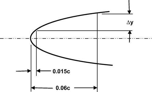
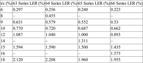
In order to facilitate the airfoil selection process several airfoil characteristics are presented here. The stall characteristics of airfoils have been correlated by an airfoil leading edge sharpness parameter Δy which is shown in Figure 5.9. The value of Δy increases (linearly) with airfoil thickness ratio and depends upon the NACA airfoil family as given in Table 5.2. Similarly the leading edge radius (LER) for a number of selected airfoils in the NACA 6-series is presented in Table 5.3.
Leading Edge Sharpness Parameter
| NACA Airfoil Family | LE Sharpness Parameter Δy/c |
| 63 Series | 0.221t/c |
| 64 Series | 0.205t/c |
| 65 Series | 0.192t/c |
| 66 Series | 0.183t/c |
Leading Edge Radius (LER) for Selected NACA 6-Series Airfoils
| t/c (%) | 63 Series LER (%) | 64 Series LER (%) | 65 Series LER (%) | 66 Series LER (%) |
| 6 | 0.297 | 0.256 | 0.240 | 0.223 |
| 8 | – | 0.455 | – | – |
| 9 | 0.631 | 0.579 | 0.552 | 0.53 |
| 10 | 0.770 | 0.720 | 0.687 | 0.662 |
| 12 | 1.087 | 1.040 | 1.000 | 0.893 |
| 14 | – | – | 1.311 | – |
| 15 | 1.594 | 1.590 | 1.500 | 1.435 |
| 16 | – | – | – | 1.575 |
| 18 | 2.120 | 2.208 | 1.960 | 1.955 |
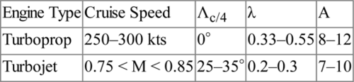
Values of α0, cm,0, cl,α, xac/c, αcl,max, cl,max, and α0, for selected airfoils were listed in Table 5.1. The values of cm,0 are observed to increase significantly with the design lift coefficient (the fourth digit in the 6-series airfoil) and these large negative values are to be avoided in the high-speed designs because they tend to put the aircraft in a dive and/or cause the wing to twist to negative angles of attack. A design lift coefficient of 0.2 is preferred to one of 0.4 for this reason. For airfoil selection purposes Abbott et al. (1945) and Abbott and Von Doenhoff (1959), as well as Hoak et al. (1978), may be consulted. An initial airfoil selection should be made before proceeding further and the value of cl,max corresponding to M = 0.2, Rec = 9 × 10⁶, and smooth surface condition noted. On the basis of the market survey and the results of Chapter 4 one may also select the wing aspect ratio A, the taper ratio λ, and the sweepback angle of the quarter chord line Λc/4. Table 5.4 provides some suggested guidelines for the current stage of the design process. Table 5.5 contains information on wing characteristics for several operational airliners of different type.
Guidelines for Wing Configurations
| Engine Type | Cruise Speed | Λc/4 | λ | A |
| Turboprop | 250–300 kts | 0° | 0.33–0.55 | 8–12 |
| Turbojet | 0.75 < M < 0.85 | 25–35° | 0.2–0.3 | 7–10 |
Wing Data for Several Operational Airlinersa
| Manufacturer | Aircraft | A | Sweep Λc/4 (deg) | Taper λ (deg) | MAC cMAC (ft) | Root (t/c)r | Tip (t/c)t | Dihedral (deg) | Incidence (deg) |
| Bombardier | Q100 | 12.4 | 0.00 | 0.50 | 6.91 | 0.18 | 0.13 | 2.5b | |
| P.R. of China | Y-7 | 11.4 | 6.8b | 0.37 | 8.15 | −2.2b | 3.00 | ||
| Avions de T.R. | ATR72-500 | 12.0 | 3.1b | 0.50 | 6.30 | 0.18 | 0.13 | 1.5b | 2.00 |
| Embraer | ERJ145LR | 7.86 | 22.8 | 0.25 | 7.03 | 5.5 | |||
| Bombardier | CRJ200LR | 8.28 | 24.5 | 0.20 | 7.00 | 0.13 | 0.10 | 2.3 | 3.40 |
| Bombardier | CRJ700ER | 7.87 | 26.0 | 0.25 | 6.60 | 2.0 | |||
| Embraer | E175 | 9.28 | 25.5 | 0.25 | 10.60 | 5.0 | |||
| Boeing | B737-700ER | 10.3 | 25.0 | 0.22 | 13.50 | 6.0 | |||
| Airbus | A320-200 | 9.35 | 25.0 | 0.23 | 13.32 | 0.15 | 0.11 | 5.1 | |
| Airbus | A310-300 | 8.79 | 28.0 | 19.10 | 0.21 | 0.11 | 4.0 | ||
| Boeing | B767-200ER | 7.99 | 31.5 | 0.22 | 22.00 | 0.15 | 0.10 | 6.0 | 4.25 |
| Boeing | B777-200 | 8.68 | 31.5 | 0.20 | 26.00 | 8.0 | |||
| Airbus | A340-300 | 10.1 | 30.0 | 0.25 | 26.90 | 0.15 | 0.11 | 5.5 | |
| Boeing | B747-400 | 7.91 | 37.5 | 0.24 | 30.60 | 0.13 | 0.08 | 7.0 | 2.00 |
| Airbus | A380-800 | 7.53 | 35.8 | 0.20 | 40.33 | 0.15 | 0.12 | 5.4 |
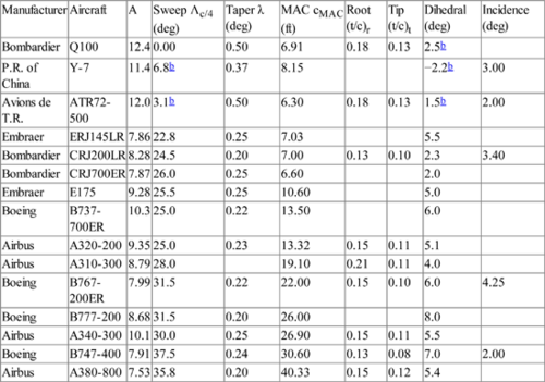
a Data taken mainly from Jane’s (2010) and manufacturers' specifications.
5.2.4 Compressibility effects on airfoils
Consider a typical high-speed NACA airfoil, the 642-015, a symmetric section with 15% thickness. The theoretical inviscid surface velocity distribution, as given in Abbott and von Doenhoff (1959), is shown in Figure 5.10. Two distributions are illustrated, one for zero angle of attack where cl = 0, and one for a moderate angle of attack where cl = 0.22. Because the section is symmetric, the zero angle of attack case has exactly the same velocity distribution on both the upper and lower surfaces. As a result the pressure distributions are identical on both surfaces and therefore the net lift is zero. However, in the moderate angle of attack case the upper surface of the airfoil has a consistently higher velocity on the upper surface than on the lower surface, resulting in lower pressures on the upper surface than on the lower surface, thereby producing a net lift force. Note that the square of the velocity is plotted since this quantity is proportional to the pressure; the difference between the upper and lower surface curves is basically the net pressure force.
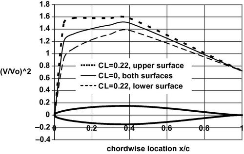
Figure 5.10 Theoretical velocity distribution on upper and lower surfaces of an NACA 642-015 symmetric airfoil for zero lift and moderate lift angles of attack.
In the lifting case shown in Figure 5.10, the upper surface velocity V is approximately 26% greater than the free stream velocity V0. Therefore as the free stream Mach number approaches 0.8, the velocity on the upper surface approaches the sonic value, i.e., M = 1. Thus the surface of the airfoil starts to feel compressibility effects before the free stream might suggest they are important. We may define the critical Mach number for an airfoil as that free stream Mach number at which the velocity at some point on the surface of the airfoil reaches the sonic value. For the airfoil considered the critical Mach number Mcrit = 0.71 for cl = 0 and Mcrit = 0.66 for cl = 0.22. Abbott et al. (1945) present graphs of Mcrit as a function of airfoil lift coefficient for a wide variety of NACA airfoils; an extract of these data for NACA 6-series airfoils is presented in Appendix D. We will make use of this material to estimate drag in Chapter 9.
Research into means of delaying the onset of compressibility effects led to the development of the “supercritical” airfoil by Richard Whitcomb, a NASA researcher who also pioneered the “area rule” that prompted a “coke-bottle” shape for fuselages that reduced transonic drag (Whitcomb and Clark, 1965) that will be discussed in Chapter 9. Because speed is of importance in air transport, modern airliners are designed to cruise as close as possible to the local sonic speed without incurring an undue drag penalty. Though there is continuing interest in traveling even faster than sound, the generation of ground-level pressure disturbances (“sonic booms”) limited the supersonic portions of flight of the Concorde supersonic transport to areas over the sea. As a consequence, supersonic transports are very specialized vehicles and their design is outside the scope of this book. As was just pointed out, flight at Mach numbers above 0.65 is likely to result in regions of supersonic flow developing over the wing. The deceleration of the supersonic flow to subsonic values over the aft sections of the wing produces shock waves which disturb the boundary layer flow there and can cause substantial flow separation with the concomitant penalty of increased drag. A schematic illustration of the flow field and pressure distributions over conventional and supercritical airfoils, as presented and discussed in detail by Harris (1990), is shown in Figure 5.11.
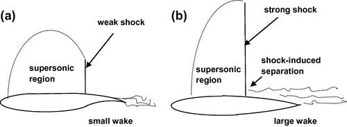
Figure 5.11 The flow field over (a) a supercritical airfoil and (b) a conventional airfoil; from Harris (1990).
Therefore, to improve performance in the low-transonic-speed range, 0.7 < M < 1, the region of locally supersonic flow over an advanced design airfoil must develop in a manner that ensures the terminating normal shock is weak, rather than the strong shock typical of conventional airfoils, like the NACA 6-series. Advanced airfoils include Whitcomb’s supercritical airfoils (Whitcomb and Clark, 1965) and Pearcy’s peaky airfoils (Pearcy, 1962), the generic shapes of which are shown in Figure 5.12. A comparison presented by Morrison (1976) of the typical chordwise pressure coefficient distribution over supercritical airfoils of the Pearcy “peaky” and Whitcomb type is shown in Figure 5.13.
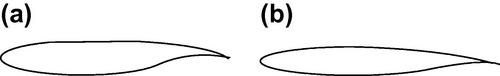
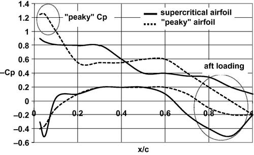
Figure 5.13 Comparison of the typical chordwise pressure coefficient distribution of supercritical airfoils of the Pearcy “peaky” and Whitcomb types.
The “peaky” airfoil is so called because it is designed to have a high suction peak near the rather slender nose of the airfoil. It is seen in Figure 5.13 that the negative of the pressure coefficient ![]() climbs rather rapidly and then settles to a relatively constant value over the middle of the chord. Note that it is common to display the negative of the pressure coefficient, −Cp, along the positive y-axis so the initial pressure actually drops rapidly. The critical value of Cp,crit, where the local Mach number on the airfoil M = 1 and p = p*, for the peaky airfoil shown is Cp,crit ∼ 0.6. Therefore, the peaky airfoil is shocking down from a relatively low locally supersonic Mach number resulting in a terminating normal shock that is weak, as desired. For the Whitcomb-type airfoil the critical value shown is Cp,crit ∼ 0.5 and once again the airfoil is shocking down from a relatively low local Mach number keeping the resulting normal shock weak. In Figure 5.13 the Whitcomb-type airfoil has cl ∼ 0.6 at M = 0.78 and the peaky airfoil has cl ∼ 0.4 at M = 0.75.
climbs rather rapidly and then settles to a relatively constant value over the middle of the chord. Note that it is common to display the negative of the pressure coefficient, −Cp, along the positive y-axis so the initial pressure actually drops rapidly. The critical value of Cp,crit, where the local Mach number on the airfoil M = 1 and p = p*, for the peaky airfoil shown is Cp,crit ∼ 0.6. Therefore, the peaky airfoil is shocking down from a relatively low locally supersonic Mach number resulting in a terminating normal shock that is weak, as desired. For the Whitcomb-type airfoil the critical value shown is Cp,crit ∼ 0.5 and once again the airfoil is shocking down from a relatively low local Mach number keeping the resulting normal shock weak. In Figure 5.13 the Whitcomb-type airfoil has cl ∼ 0.6 at M = 0.78 and the peaky airfoil has cl ∼ 0.4 at M = 0.75.
Thus all supercritical airfoil designs are marked by controlling the supersonic flow region so as to produce weak terminal shocks, but Whitcomb’s airfoil is seen to have substantial aft loading, as pointed out in Figure 5.13, due to the lower surface reflex curvature near the trailing edge. The Whitcomb-type supercritical airfoil combines the geometrical features of a rounder leading edge, flatter upper surface, and more reflexed trailing edge as compared to the “peaky” type of airfoil developed by Pearcy. These design differences reduce the leading edge pressure coefficient “peakiness,” extend the near sonic flow further aft on the airfoil, and yield a more highly loaded aft portion of the airfoil. The result is a somewhat higher lift coefficient developed at a higher free stream drag divergence Mach number.
As mentioned previously, the supercritical airfoil has a flatter upper surface designed to provide a smoother deceleration of the supersonic flow so that a weaker shock wave is produced than on a conventional airfoil. A family of NASA SC-series supercritical airfoils is shown in Figure 5.14. Note that the airfoil shape, when flipped vertically, bears a resemblance to that of a conventional airfoil.
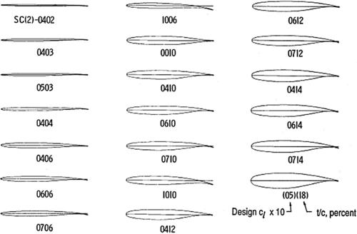
Figure 5.14 A family of NASA supercritical (SC) airfoils; from Harris (1990).
The extent of drag reduction possible is shown in Figure 5.15(a) for an 11% thick supercritical airfoil, and a 12% thick conventional NACA 641-212 low-drag airfoil. The major improvement provided by the supercritical airfoil design is found to be in delaying the onset of the drag divergence Mach number from MDD = 0.7 for the conventional airfoil to MDD = 0.8 for the supercritical airfoils. There are some additional benefits of the supercritical airfoil in that the lift is preserved and even augmented at the higher free stream Mach numbers possible. This is shown in Figure 5.15(b) where the normal force coefficient for the supercritical airfoil and the NACA 641-212 conventional airfoil is shown as a function of free stream Mach number.
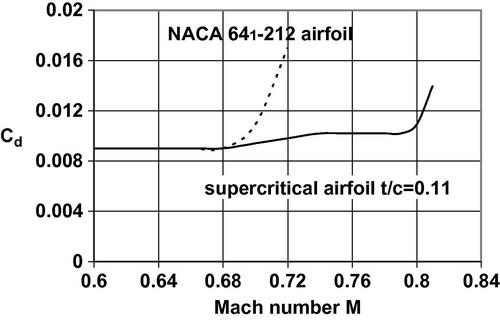
Figure 5.15(a) Drag coefficients as a function of Mach number for a supercritical airfoil and a conventional airfoil; from Harris (1990).
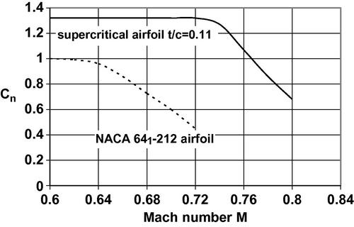
Figure 5.15(b) The normal force coefficients for a supercritical and a conventional airfoil as a function of free stream Mach numbers; from Harris (1990).
However, there is an increase in pitching moment, not shown in Figure 5.15(b), that turns out to be not as much of a trim drag penalty for swept-wing aircraft fitted with supercritical airfoils because the optimum wing twist increases as the Mach number increases. This increased wing twist alleviates the penalty arising from increased pitching-moment coefficient.
The drag divergence Mach number is defined as that Mach number where the derivative of the drag coefficient with respect to Mach number has a particular value; NASA uses 10% as its criterion, i.e., dcd/dM = 0.10. Thus the use of supercritical airfoils on the wings of modern airliners has provided substantial performance increases. So-called “peaky” airfoils, described previously, began to see operational use on several aircraft, including McDonnell Douglas DC-9 Series 30, DC-8 Series 63, and DC-10 Series 10. Then first-generation Whitcomb-type supercritical airfoils were introduced on airliners like the Airbus A300-600, A310-300, and the Boeing 767-200, while next-generation versions were used on the Bombardier CRJ 200 LR, the Embraer EMB-145, and the Airbus A321-200 and A340-300. Wing designs are so valuable that aircraft manufacturers consider them proprietary and detailed information on them is not readily available. Schiktanz and Scholz (2011) present a compilation of wind tunnel test data on supercritical airfoils taken from publically available reports, as presented in Table 5.6(a). They noted that conventional NACA laminar flow airfoils showed good characteristics at supercritical speeds and included the NACA 651-213 studied by Plentovich et al. (1984) in their survey. The issue of the transonic drag reductions possible with supercritical airfoils will be treated in detail in Chapter 9.
Supercritical Airfoils Compiled by Schiktanz and Scholz (2011)
| Airfoil | (t/c) max% | References |
| BAC 1 | 10 | Johnson and Hill (1985) |
| CAST 7 | 11.8 | AGARD (1979) |
| CAST 10-2/DOA 2 | 12.1 | Dress et al. (1984) |
| Cessna EJ | 11.5 | Allison and Mineck (1996) |
| DFVLR R4 | 13.5 | Jenkins, Johnson, Jr., Hill, et al. (1984) |
| NLR 7301 | 16.3 | AGARD (1979) |
| NPL 9510 | 11 | Jenkins (1983) |
| SC(2)-0012 | 12 | Mineck and Lawing (1987) |
| SC(2)-0710 | 10 | Harris (1975a) |
| SC(2)-0714 | 14 | Harris (1975b); Harris et al. (1980) |
| SC(3)-0712(B) | 12 | Johnson et al. (1985) |
| SKF 1.1 | 12.07 | AGARD (1979) |
5.2.5 Computational resources for airfoil analysis and design
As is evident from the material presented in the previous sections, there is a broad and diverse literature on airfoils and their characteristics. The approach taken in this book is to make expedient use of extant data and empirical methods based on theory and extensive experience in order to arrive at reasonably accurate design solutions for the many components of the complex system that is a modern commercial aircraft. The theoretical background on the aerodynamics of airfoils is described in Appendix C along with some of the techniques which may be used to calculate the flow field around airfoils. The availability of increasingly powerful personal computers has encouraged the development of a wide range of software applicable to various aspects of airplane design. In the case of airfoils alone, UIUC (2013) maintains a readily accessible library of almost 1600 airfoil designs and provides information on geometry and performance. They also provide links to several of the application codes that have proven to be successfully used by students, for example, XFOIL, developed by Drela (1989) and released under the GNU general public license. Public domain software provided by PDAS (2013) includes PABLO, an airfoil analysis program with boundary layer analysis. An online search will reveal a number of other codes for airfoil analysis and development.
For the present purpose of learning the basic principles of commercial aircraft design it seems prudent to determine the lifting characteristics of the design project airplane by simply using the reported characteristics of the NACA 6-series or SC-series airfoils. It is common for substantial time to be expended in learning how to use various software packages, and this effort often intrudes on the total time available for the entire project. As one gains more understanding of the aerodynamics involved and experience in assessing the results of various analyses it becomes expeditious to incorporate more complete theoretical tools.
5.3 Lifting characteristics of the wing
The maximum lift coefficient of the airplane CL,max depends upon many factors. Only the most important of these will be considered here and they are listed below.
a. Airfoil maximum lift coefficient cl,max.
b. Wing aspect ratio A, taper ratio λ, and sweepback angle Λ.
c. Trailing edge flap design and deflection angle.
d. Leading edge flap design and deflection angle.
The methods that will be used to estimate CL,max for the various configurations of a wing are taken mainly from the USAF Stability and Control DATCOM, Hoak et al. (1978) and are empirical in nature. There are other, more sophisticated, approaches based on different computational fluid dynamics (CFD) schemes which will be discussed in varying degrees of detail. Such scientifically richer methods will generally have been covered in the fluid dynamics analysis courses of an engineering degree program and may be implemented, if desired. However, it is important to develop some familiarity with empirical and approximate techniques rarely covered in academic courses. The rapid turnaround they provide is of great value in preliminary design situations in industry.
5.3.1 Determination of the wing lift curve slope
The airfoil characteristics described thus far are based on two-dimensional flow whereas wings have finite span and three-dimensional effects must be considered. Basic wing theory and analysis is presented in Appendix C. This background material on wings should be reviewed to complement the mainly empirical approaches presented here. The three-dimensional lift curve slope of conventional wings CLα is given, per radian, by the following equation:
Thus CLα is a function of wing aspect ratio, mid-chord sweep angle Λc/2, Mach number, and airfoil section (defined parallel to the free stream) lift curve slope. The factor κ in the figure is the ratio of the experimental two-dimensional (i.e., airfoil) lift curve slope (per radian) at the appropriate Mach number (cla)M to the theoretical value at that Mach number, 2π/β, or κ = (clα)M/(2πβ). Note that the theoretical (Prandtl-Glauert) correction for subsonic compressibility is (clα)M = clα/β, so in the absence of an experimental value for (clα)M the value for κ = clα/2π, that is, the ratio of the actual low-speed airfoil lift curve slope to that of the airfoil in ideal incompressible flow will suffice. The section lift curve slope (per degree) is obtained from Table 5.1 or from, for example, Hoak et al. (1978), and β is the Prandtl-Glauert factor
The sweep-conversion formula, Equation (5.11), may be used to find the mid-chord sweep for any straight-tapered wing as follows:
Recall that λ is the taper ratio, ct/cr. Writing Equation (5.11) to find the sweepback angle of the leading edge from that at any other constant percent chord line (n = %c/100), for trapezoidal wing planforms, yields
For example, if the quarter chord sweepback angle is known (n = 1/4 = 0.25), the sweepback angle of the leading edge is easily determined. In a similar fashion, once the sweepback angle of the leading edge is known, the sweepback angle of any other constant percent chord line can be easily found:
5.3.2 Sample calculation of the wing lift curve slope
Consider the 64A010 airfoil, a symmetric section of thickness ratio t/c = 10% being used in a wing with an aspect ratio A = 5, a leading edge sweepback Λ = 46.6o, and a taper ratio λ = 0.565. To find the lift curve slope of this wing at a Mach number M = 0.4 we may use Equation (5.18). First we must determine the sweepback of the half-chord line, which may be found using Equation (5.22):

We also require the value of κ = (clα)M/(2π/β). Because (clα)M, the experimental value for clα at M = 0.4, is not provided here, we approximate it by clα/β, where clα = 0.110/° (=6.303 per radian) is the low-speed value given in Table 5.1. Then Equation (5.18) yields
This result, CLα = 3.48 per radian, may also be written as CLα = 3.48/57.3 = 0.061 deg−1. This is about 1.7% higher than the experimental result of Johnson and Shibata (1951) which is CLα = 0.060 deg−1. If we increase the Mach number to M = 0.8, then CLα = 0.068 deg−1, which is about 3.9% higher than the reported result of 0.0654. We see that the lift curve slope of the finite wing is substantially less than that of the airfoil of which it is comprised. However, note that doubling the Mach number from 0.4 to 0.8 increases the lift curve slope of the wing by almost 10%.
5.4 Determination of wing maximum lift in the cruise configuration
Section 4.1.3.4 of DATCOM (Hoak et al., 1978) presents methods of rapidly estimating the maximum lift and angle of attack for wings at subsonic, transonic, supersonic, and hypersonic speeds. The material pertinent to subsonic speed is used in the current design approach. At subsonic speeds a distinction is made between low- and high-aspect-ratio wings. The maximum lift of high-aspect-ratio wings at subsonic speeds is directly related to the maximum lift of the wing airfoil sections. Wing planform shape does influence the maximum lift obtainable, but its effect is distinctly subordinate to the influence of the section characteristics. For low-aspect-ratio wings, like fighter plane delta wings or the ogee wing of the Concorde SST, the maximum lift is primarily related to planform shape, while the airfoil section characteristics are secondary. Because commercial airliners are characterized by high-aspect-ratios only the portion of the DATCOM method pertinent to such wings is presented here. Other methods for calculating maximum lift, usually involving additional complexity but with increased accuracy are also covered in this section and may be used for a collective comparison.
5.4.1 Subsonic maximum lift of high-aspect-ratio wings
The maximum lift and stalling characteristics of high-aspect-ratio wings, are, to a first approximation, determined by section properties which, for selected NACA 6-series sections, have been presented in Table 5.1. See Section 4.1.1.4 of DATCOM (Hoak et al., 1978), for methods for dealing with non-standard airfoils. Obviously, three-dimensional effects arising from tip, taper, or sweepback effects have an influence on the stalling characteristics of a wing. As a result, the stall of a wing, even a simple unswept, untwisted wing using a constant airfoil sections, starts at a specific angle of attack at a particular point on the wing and then rapidly spreads across the span as the angle of attack increases further. Highly tapered or swept back wings tend to stall near the tips, while wings with little sweep or taper tend to stall near the root. As a first step in the process of accounting quantitatively for the existence of this effect in swept-wing design, it is necessary to examine the nature of the separation process which limits cl,max for the two-dimensional (airfoil) and three-dimensional (wing) cases.
On thick or highly cambered airfoils separation begins at the trailing edge and spreads upstream as the angle of attack increases, finally fixing cl,max. The typical pressure distribution on the upper surface shows a sharp peak near the leading edge and an area of constant pressure over the aft portion where separation exists. On very thin airfoils the flow separates from the surface starting at the leading edge but then reattaches to the surface farther aft. This point of reattachment moves downstream as the angle of attack increases and finally fixes cl,max when it reaches the trailing edge. The pressure distribution on the upper surface shows a slight peak near the leading edge followed by relatively constant pressure region up to the point of reattachment, and then recovery to essentially free stream pressure. Intermediate- thickness airfoils with about 10-percent thickness and little camber typically have both types of separation simultaneously. The value of cl,max is fixed when the trailing edge separation nears or reaches the point of reattachment of the leading edge separation. The pressure distribution on the upper surface in this case shows little or no sharp peak near the leading edge and lack of recovery to the free stream value at the trailing edge.
On the basis of these distinctions and from examination of the chordwise pressure distributions just prior to stall of a given airfoil section in two- and three-dimensional flow, an insight can be had into the mechanism by which sweepback provides a degree of natural boundary layer control. Harper and Maki (1964) discuss the case of a wing swept back at 45°. The two-dimensional pressure distributions for the airfoil used in the wing show evidence of both leading and trailing edge types of separation discussed above. This same type of separation pattern is found in the three-dimensional flow over the outboard region of the swept wing. However, on the inboard sections the separation pattern changes to the thin airfoil, leading edge type of separation. From this, it is concluded that as the root is approached from the tip, the spanwise flow due to sweep becomes increasingly effective in controlling the boundary layer resulting in suppression of the trailing edge type of separation of the swept wing.
The two major effects of wing sweep may be said to be:
• suppression of inboard stall, particularly at the trailing edge, through the natural boundary layer control just discussed,
• outboard movement of the peak of the span loading distribution, which increases as taper is increased.
These two factors combine to produce a stalling pattern which is unlike that commonly experienced by unswept wings.
It must be recognized that the maximum lift of the wing alone, as given in this section, may be substantially altered by interference effects. The addition of fuselages, nacelles, pylons, and other protuberances can change the aerodynamic characteristics of a given configuration near the stall. Interference effects of this type are discussed in Section 4.3.1.4 of Hoak et al. (1978).
5.4.2 DATCOM method for untwisted, constant-section wings
We will consider high-aspect-ratio wings, defined as those with an aspect ratio
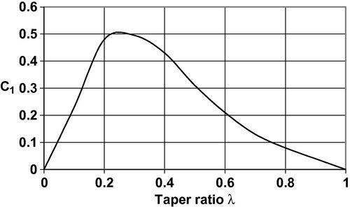
The quantity C1 is a correlation factor that depends on the taper ratio λ; a graph of C1 as a function of λ is shown in Figure 5.16.
An empirically derived method, based on experimental data, for predicting the subsonic maximum lift and the angle of attack for maximum lift of high-aspect-ratio, untwisted, constant-section (symmetrical or cambered) wings is given. The development follows the DATCOM method (Hoak et al., 1978). The equations and directions for using the charts are as follows:
The first term on the right-hand side of Equation (5.24) is the maximum lift coefficient at M = 0.2 and the second term is the lift increment to be added for Mach numbers between 0.2 and 0.6. Here ![]() is obtained from Figure 5.17 and
is obtained from Figure 5.17 and ![]() is the section maximum lift coefficient at M = 0.2 obtained from Table 5.1. The quantity
is the section maximum lift coefficient at M = 0.2 obtained from Table 5.1. The quantity ![]() is a Mach number correction obtained from Figure 5.18. For cruise Mach numbers greater than 0.6, no general empirical correlation is readily available, so reasonable extrapolation to the cruise Mach number may be carried out. This is acceptable for preliminary design purposes because flight under normal conditions will not involve maximum lift at the cruise speed. However, the more accurate methods for wing lift given in Appendix C and used subsequently in this chapter can accommodate the high subsonic cruise speeds of modern airliners. In Equation (5.24)
is a Mach number correction obtained from Figure 5.18. For cruise Mach numbers greater than 0.6, no general empirical correlation is readily available, so reasonable extrapolation to the cruise Mach number may be carried out. This is acceptable for preliminary design purposes because flight under normal conditions will not involve maximum lift at the cruise speed. However, the more accurate methods for wing lift given in Appendix C and used subsequently in this chapter can accommodate the high subsonic cruise speeds of modern airliners. In Equation (5.24) ![]() is the wing lift curve slope for the Mach number under consideration, obtained previously from Equation (5.18) and
is the wing lift curve slope for the Mach number under consideration, obtained previously from Equation (5.18) and ![]() is the wing zero-lift angle of attack. Sharpes (1985) suggests that the zero-lift angle of attack for swept wings as calculated by DATCOM tends to overestimate the experimentally observed angles and should be replaced by an improved correlation given as follows:
is the wing zero-lift angle of attack. Sharpes (1985) suggests that the zero-lift angle of attack for swept wings as calculated by DATCOM tends to overestimate the experimentally observed angles and should be replaced by an improved correlation given as follows:
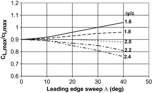
Figure 5.17 Variation of CL,max/cl,max with leading edge sweep for different values of the airfoil leading edge sharpness parameter Δy/c (Hoak et al., 1978).
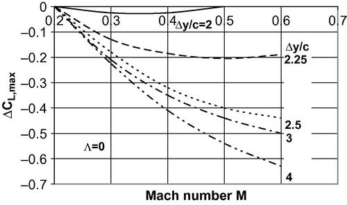
Figure 5.18(a) Mach number correction for maximum wing lift for various values of the airfoil leading edge sharpness parameter Δy/c and leading edge sweep Λ = 0° (Hoak et al., 1978).
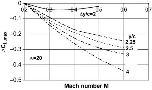
Figure 5.18(b) Mach number correction for maximum wing lift for various values of the airfoil leading edge sharpness parameter Δy/c and leading edge sweep Λ = 20° (Hoak et al., 1978).
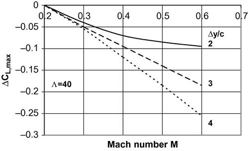
Figure 5.18(c) Mach number correction for maximum wing lift for various values of the airfoil leading edge sharpness parameter Δy/c and leading edge sweep Λ = 40° (Hoak et al., 1978).
The angle of attack for zero sweep αΛ = 0 is equivalent to the airfoil zero-lift angle of attack, again for the Mach number under consideration, and may be obtained from Table 5.1. The angle of attack increment ![]() is obtained from Figure 5.19. The leading edge parameter Δy, which does not explicitly appear in the equations, must be used in reading values from the charts. The value of Δy is expressed in percent chord and is obtained from Table 5.2. In calculating
is obtained from Figure 5.19. The leading edge parameter Δy, which does not explicitly appear in the equations, must be used in reading values from the charts. The value of Δy is expressed in percent chord and is obtained from Table 5.2. In calculating ![]() the value of CLmax calculated from Equation (5.18) is used as the numerator of the first term of Equation (5.24).
the value of CLmax calculated from Equation (5.18) is used as the numerator of the first term of Equation (5.24).
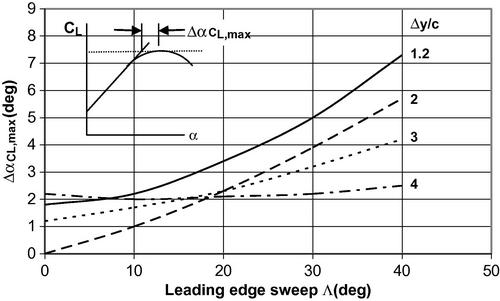
Figure 5.19 Angle of attack increment (defined in inset) for wing maximum lift in subsonic flight (Hoak et al., 1978).
5.4.3 Sample calculation for an untwisted, constant-section wing
Consider the case of a swept wing with an NACA 64A010 airfoil, a quarter-chord sweep Λc/4 = 45o, taper ratio λ = 0.568, and aspect ratio A = 5 operating at M = 0.4 and a chord-based Reynolds number Rec = 2 million. The leading edge sweepback may be found by using Equation (5.21) as follows

Then ΛLE = 46.65o and the inequality of Equation (5.23) is satisfied because Figure 5.16 yields C1 = 0.24, therefore
Thus the high-aspect-ratio requirement is met and the DATCOM approach of Section 5.4.2 may be applied. The maximum lift coefficient for the airfoil section may be found from Table 5.1 to be cl,max = 1.23. The leading edge thickness parameter for the NACA 64-series airfoils is taken from Table 5.2 to be (Δy/c) = 0.205(t/c) and this may be used in Figure 5.17 (extrapolating out to ΛLE = 46.65°) to estimate CL,max/cl,max = 0.85. Similar extrapolation using Figure 5.18 permits one to estimate ΔCLmax = −0.53. Then Equation (5.24) yields

This result is 4.2% higher than the experimental result of 0.95 for this case, as reported by Johnson and Shibata (1951). The angle of attack increment for maximum lift may be estimated from Figure 5.19 as ΔαCLmax = 7°. Then the angle of attack for maximum lift is obtained from Equation (5.25) as
The zero-lift angle of attack for this symmetric airfoil is given in Table 5.1 as α0 = 0 and the lift curve slope was previously calculated as CLα = 0.061 in Section 5.3.1. This empirically calculated result of 23.3° is 3.3% lower than the experimental result of 24° for this case reported by Johnson and Shibata (1951).
5.4.4 Maximum lift of unswept twisted wings with varying airfoil sections
High-aspect-ratio wings are often slightly twisted along a spanwise axis and may have varying airfoil sections along the span in order to obtain favorable stalling characteristics. Abbott and von Doenhoff (1959) suggest that a reasonable estimate for the maximum lift of the wing, that is, the stall point, is given by location on the span where the local section lift coefficient of the wing is equal to the maximum lift coefficient of the airfoil used at that station. Though this estimate has no strong theoretical justification it is also given as the preferred method by DATCOM. Of course, this approach requires the availability of a span loading method which can supply the variation of the local lift coefficient with spanwise coordinate. Some simple lifting line and lifting surface methods for estimating the span loading are described in detail in Appendix C and various sample problems are addressed there. The simple approach for estimating the maximum lift of the wing may be described as follows:
1. Using any appropriate theoretical span loading method, as discussed in Appendix C, plot the calculated section lift coefficient cl as a function of spanwise position η = y/(b/2) and angle of attack α.
2. Plot the section lift coefficient cl,max for the airfoil section(s) used on the given wing as a function of spanwise station for the appropriate Reynolds number and Mach number.
3. The angle of attack and spanwise position for maximum lift is approximated by the angle of attack at which the curves of steps 1 and 2 become tangent.
The integrated value of the curve of step 1 approximates the maximum lift coefficient of the wing. For example, the analysis in Appendix C for an unswept wing with aspect ratio A = 7 and taper ratio λ = 0.5 results in the spanwise distribution of local lift coefficient shown in Figure 5.20. Assuming that an NACA 632-215 airfoil is used throughout the span of the wing, the data of Abbott and Von Doenhoff (1959) show a two-dimensional maximum lift coefficient of cl,max = 1.6 at α = 16° for a smooth finish airfoil in the Reynolds number range 6 × 10⁶ < Rec < 9 × 10⁶. Such an airfoil is appropriate for an unswept wing on a turboprop aircraft taking off at about 130 kts (M = 0.2) at sea level and flying at a cruise speed of 300 kts (M = 0.5) at 25,000 ft altitude. If the wing under consideration has a typical value for the mean aerodynamic chord of cMAC = 10 ft, the root chord is cr = 12.86 ft and the tip chord is ct = 6.43 ft. Then at takeoff the Reynolds number varies linearly from 18 million at the root to 9 million at the tip. Similarly, in cruise the Reynolds number varies linearly from 20.6 million at the root to 10.3 million at the tip. Based on the discussion at the beginning of Section 5.2 we assume there is little change in cl,max from its value at Rec = 9 million and therefore cl,max may be considered constant along the span. In Figure 5.20 this value of cl,max = 1.6 is approximately tangent to the calculated local lift coefficient at a spanwise location η ∼ 0.6 and the DATCOM method being employed suggests that stall will originate at or near that spanwise station. The lifting surface result for the wing lift coefficient is found to be CL = 1.50 at α = 17.7° which is actually slightly larger than the airfoil stall angle.
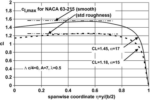
Figure 5.20 Spanwise distribution of the local lift coefficient for an unswept wing with A = 7 and λ = 0.5 at two angles of attack. Also shown is the maximum lift coefficient for an NACA 632-215 airfoil with smooth and standard roughness surface.
If instead of a smooth finish the NACA 632-215 airfoil used throughout the span of the wing has the standard roughness finish, the two-dimensional maximum lift coefficient is given as cl,max = 1.25 at α = 15° at a Reynolds number of 6 × 10⁶. As mentioned at the beginning of Section 5.2 the maximum lift coefficient of an airfoil appears to be insensitive to Reynolds number if the boundary layer over the airfoil is turbulent everywhere beyond the immediate region of the leading edge. Therefore we expect the line cl,max = 1.25 to be constant over the entire span and find that, once again, it is approximately tangent to the calculated local lift coefficient at a spanwise location η ∼ 0.6. The DATCOM method then suggests that the wing stall will originate at or near that spanwise station. The lifting surface result for wing lift coefficient is CL = 1.185 at α = 15° which is equal to that of the airfoil stall angle.
5.4.5 Reynolds number in flight
The Reynolds number based on the chord length may be written in terms of the Mach number V/V* as follows:
Using the information on the atmosphere presented in Appendix B, one may determine the ratio V*/ν as a function of altitude and then show that Rec/Mc = 7 × 10⁶exp(−z/32,000), where z is the altitude in feet, represents a good fit to the atmospheric data. For typical commercial aircraft applications the Reynolds number per foot of chord length lies between 1.5 and 2 million per foot, as illustrated in Figure 5.21. Note that for the major operations of takeoff and cruise, the unit Reynolds numbers for turboprop and turbofan airliners fall in the range of 1.5–2 million per foot. The data given in Table 5.5 show that the mean aerodynamic chord for turboprop aircraft lies in the range 6.9 ft < cMAC < 10.6 ft and for turbofan airliners in the range of 13.3 ft < cMAC < 26.9 ft, while for very large aircraft the range is 30.6 ft < cMAC < 40.33 ft. Thus the actual Reynolds number based on mean aerodynamic chord is 10–20 million for turboprop airliners, 20–54 million for turbofan airliners, and 45–80 million for very large aircraft like the B747 and A380. Note that for highly tapered wings the outboard chords may be considerably smaller than the mean aerodynamic chord and will experience lower Reynolds numbers. For example, with a taper ratio λ = 0.4 the tip chord ct ∼ 0.4cMAC. During low-speed operations like landing and takeoff, high lift devices such as flaps and slats are deployed. Because the characteristic lengths of these elements are considerably smaller than the local wing chord they will be operating at lower Reynolds number and therefore more susceptible to flow separation and stalling.
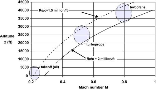
Figure 5.21 The variation of unit Reynolds number Re/cMAC is shown for typical commercial aircraft applications.
In the limited Reynolds number range achieved for the smooth NACA airfoils, 3 × 10⁶ < Rec < 9 × 10⁶, the maximum lift coefficient has its lowest value at 3 × 10⁶ and then increases to a constant value for Reynolds numbers of 6 × 10⁶ and 9 × 10⁶. The general trend is for cl,max to increase slowly, if at all, with increases in Reynolds number and for that increase to be more substantial for thicker sections. This is understandable because as the Reynolds number increases the boundary layer effects become relatively weaker allowing the flow to remain attached to the airfoil for longer distances along the airfoil surface. The lift of an airfoil depends primarily on keeping the flow attached to the airfoil while friction drag itself weakly influences the lift of an airfoil. However, little experimental data are available at higher Reynolds numbers, being limited to about 25 million in the traditional variable-density wind tunnels, but rising to as much as 100 million in cryogenic wind tunnels, as previously described in Section 5.2.2.
5.4.6 Maximum lift of swept and twisted wings with varying airfoil sections
As mentioned in the previous section, Abbott and Von Doenhoff (1959) suggest that a reasonable estimate for the spanwise location at which stall is initiated is given by that spanwise station where the local section lift coefficient cl(y) for the wing first becomes equal to the maximum lift coefficient of the airfoil used. The wing lift coefficient at this condition is considered the maximum lift of the wing CL,max. The usefulness of this method is that the effects of airfoil section and wing planform may be treated independently and its success in providing reasonable estimates has been established in practice. However, as pointed out by Harper and Maki (1964), the measured maximum lift of swept wings is lower than that which would be expected based on the experience with unswept wings. They proposed that the same criterion used for unswept wings can be correctly applied to sweptback wings if two conditions are satisfied: first, that an appropriate span loading analysis is used to compute the spanwise distribution of the section lift coefficient cl(y), and second, that the concepts of simple sweep theory be used in applying two-dimensional airfoil data.
Simple sweep theory states that the section characteristics of an infinite wing are invariant with yaw angle provided that these characteristics are defined along a line normal to the line of constant chord and that the appropriate reference velocity is the component of velocity along that line. The characteristics involved include not only the inviscid pressure coefficient distributions, but also the associated boundary layer characteristics, whether laminar or turbulent. For example, an infinite wing swept at some angle Λ may be considered as an unswept wing encountering a free stream velocity of VcosΛ, as shown in Figure 5.22. The other component of the free stream velocity VsinΛ runs solely along the span and, in an inviscid flow, has no effect on the pressure field developed. The incremental lift of the wing is given by
![]()
For a given span segment of length b = b’/cosΛ the lift is constant and given by
Then the lift coefficients are related by
![]()
Because the planform area of the segment S = b’c’ = bc, the lift coefficients normal to and along the leading edge are related by
This is usually called the simple sweep theory for an infinite wing at a given angle of sweep. Obviously the flow field over a finite swept wing cannot be directly related to that over a segment of an infinite swept wing because three-dimensional effects due to the presence of a centerline and a wingtip will alter the surface pressure field in regions shown schematically in Figure 5.23.
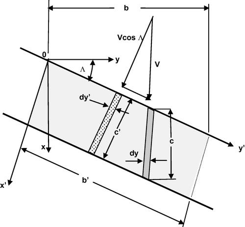
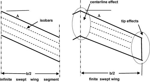
Figure 5.23 The isobars for an infinite swept wing and a finite swept wing showing the regions disturbed by three-dimensional effects.
The invariance of the pressure distributions and the laminar boundary characteristics according to simple sweep theory have been demonstrated theoretically by Jones (1947a,b). Experimental evidence supports these results and suggests that turbulent boundary layer characteristics behave in a similar manner. Harper and Maki (1964) show that the method described for predicting maximum lift of swept wings of widely varying planform and profile geometries is consistently conservative by around 20%. This conservatism suggests that the spanwise flow over swept wings provides natural boundary layer control which permits local section maximum lift coefficients to reach higher values than could be achieved in purely two-dimensional flow.
Therefore, as in the case of the unswept wing, we use an applicable span loading method which supplies the variation of the local lift coefficient with spanwise coordinate. For swept wings a lifting surface method for estimating the span loading must be used and several are described in detail in Appendix Calong with various sample problems. This approach is recommended in DATCOM for estimating the maximum lift of a swept and twisted wing and may be described as follows:
1. Using any appropriate theoretical span loading method, as discussed in Appendix C, plot the calculated section lift coefficient cl as a function of spanwise position η = y/(b/2) and angle of attack α.
2. Plot the maximum lift coefficient cl,max for the airfoil section(s) used on the given wing as a function of spanwise station for the appropriate Reynolds number and Mach number. Here the maximum lift coefficient is that appropriate to the streamwise airfoil section used in the wing. The maximum lift coefficient of the streamwise section is approximated by cl,max = (cl,Λ=0)maxcos2Λ where (cl,Λ=0)max is the maximum lift coefficient of the airfoil section normal to the leading edge. Simple sweep theory requires that the Reynolds and Mach numbers to be used are those for which the streamwise velocity V is replaced by VcosΛ and the streamwise chord length c by ccosΛ.
3. The angle of attack and spanwise position for maximum lift is assumed to be determined by the angle of attack at which the curves of steps 1 and 2 first become tangent.
Turning our attention to a turbofan airliner with a swept (Λc/4 = 30°) and twisted wing (Ω = 5°) of aspect ratio A = 8 and taper ratio 0.25 we would select a relatively thin airfoil section. The NACA 64A210 airfoil is a possible choice and, like the thicker NACA 632-215 airfoil used in the example for the unswept wing for a turboprop airliner, it also has cl,max = 1.44 for a smooth surface finish in the Reynolds number range of 6–9 million, as reported by Abbott and Von Doenhoff (1959). Such a wing would have a typical value for the mean aerodynamic chord in the range 13.3 ft < cmac < 26.9 ft. The tip chord ct = λcr and the root chord is given by
Thus cr = 1.43cmac so that typical root chord for such an airliner would lie in the range 19.0 ft < cr < 39 ft while the tip chord would be in the range of 5 ft < ct < 10 ft. For the mid-range case of cr = 30 ft and ct = 7.5 ft and using the approximation Rec/Mc = 7 × 10⁶exp(−z/32,000), the Reynolds number at takeoff (M = 0.20) would vary linearly from 10.5 million at the tip to 42 million at the root. In cruise (M = 0.8) the Reynolds number varies linearly from 14.1 million at the tip to 56.3 million at the root. Based on the discussion at the beginning of Section 5.2 we assume there is little change in cl,max from its value at Rec = 9 million and therefore cl,max may be considered constant along the span.
Applying the simple sweep approximation we set cl,max = cl,max,0(cos30°)2. We also consider that the appropriate Reynolds number in this approximation is based on c(cosΛc/4) and the appropriate Mach number is M(cosΛc/4). Then, in takeoff, the Reynolds number varies from 7.9 million at the tip to 31.5 million at the root. In cruise the Reynolds number varies linearly from 10.6 million at the tip to 42.2 million at the root. In the spanwise load distribution shown in Figure 5.24 the sweep-corrected value of cl,max = 1.44(0.866)2 = 1.08 is seen to be approximately tangent to the calculated local lift coefficient at a spanwise location η ∼ 0.6 and the DATCOM method being employed suggests that stall will originate at or near that spanwise station. The lifting surface result for the wing lift coefficient is found to be CL = 0.996 at α = 12.7°.
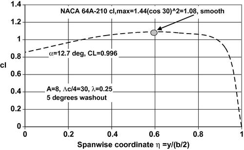
Figure 5.24 Spanwise distribution of the local lift coefficient for a swept wing with A = 8, λ = 0.25, and 5° washout at an angle of attack α = 12.7°. Also shown is the maximum lift coefficient for an NACA 64A210 airfoil with smooth surface corrected for sweep.
5.4.7 A simple modified lifting line theory for CL,max
Phillips and Alley (2007) present a method for estimating the maximum wing lift that is based on the classical lifting line theory discussed in Appendix C. Their approach involves providing correction factors for the effects of twist and sweepback on the span loading of unswept, untwisted, tapered wings. The correction factors are developed with the aid of CFD panel method computations for a variety of conventional wing planforms. Curves for the correction factors are presented for a number of specific taper and aspect ratios along with the general method for calculating these effects for other wing geometry. If we confine our attention to taper ratios in the range 0.25 < λ < 0.6, small twist angles 0 < Ω < 5°, and aspect ratios in the range 8 < A < 12, which are typical of commercial airliners, we may use the results presented by Phillips and Alley (2007) to develop the following approximations:
1. For the range of aspect and taper ratios considered here the ratio of wing lift coefficient to maximum section lift coefficient may be fitted, within an error of about 1%, by the following simple equation:
2. The sweep correction is given by Phillips and Alley as
The coefficients in this equation may be approximated by the following simple relations:
This gives errors in KLΛ less than 10% except where KΛ1<1, but in that case it has little effect on the final result for KLΛ.
3. The twist correction curves given by Phillips and Alley (2007) cover a wide range of specific wing parameters. For wing planforms of the type considered here, we may use the curves presented to provide simple estimates for the twist correction factor KLΩ, which appears in the term KLΩCL,αΩ/cl,max:
a. For turboprop airliners with 10 < A < 12 and λ ∼ 0.5 we may estimate CL,α ∼ 5 per radian, Ω ∼ 0.1 radian, and cl,max ∼ 1.6 so that CL,αΩ/cl,max∼0.31, corresponding to KLΩ ∼ 0.1.
b. For turbofans with 8 < A < 10 and λ ∼ 0.25 we may estimate CL,α ∼ 4.5 per radian, Ω ∼ 0.1 radian, and cl,max ∼ 1.6 so that CL,αΩ/cl,max ∼ 0.28, which corresponds to KLΩ ∼ −0.2.
The twist correction term has a magnitude lying in the range of 0.056 < KLΩCL,αΩ/cl,max < 0.031, with the low end of the range corresponding to low taper ratios (λ around 0.25) and the high end of the range corresponding to moderate taper ratios (λ around 0.5).
Phillips and Alley also introduce a stall factor given by
For typical values of the parameters in the second parentheses, a change of Ω from 0° to 5° results in a reduction of KΛS by between 1% and 2%.
To estimate the maximum lift coefficient of a wing these quantities may be combined according to the following relation given by Phillips and Alley (2007):
According to the order of magnitude estimate provided in item (3) above, the term in parentheses lies in the range of 1–1.033 for moderate taper ratios and to 1–0.967 for low taper ratios. Of course, as the washout is reduced the term in parentheses approaches unity.
5.4.8 Comparison of span loading and the modified lifting line methods
Applying this approach to the unswept (Λc/4 = 0), untwisted (Ω = 0) wing treated in the previous section we find from Equation (5.30) for A = 7 and λ = 0.5 that CL/cl,max = 0.937. Because the wing is unswept we find, from Equation (5.31), that KLΛ = 1. The wing is untwisted (Ω = 0) and therefore Equation (5.34) yields the stall factor KLS = 0.961. From Equation (5.35) we estimate that the maximum lift coefficient is CL,max = 0.9cl,max. For the NACA 632-215 airfoil at high Rec the section maximum lift coefficient is cl,max = 1.6 and therefore the wing maximum lift coefficient is CL,max = 1.44 at α = 17°. This compares well with the DATCOM technique applied to this wing in Section 5.4.4 where CL,max was found to be 1.49 at an angle of attack of 17.6°.
Phillips and Alley (2007) note that the stall correction factor is based on CFD studies alone and only at one Reynolds number, 3 million, which is a relatively low value for practical wings. They suggest that this correction should be applied with discretion, and probably not applied at all in preliminary studies. In this case the use of KLS = 1 leads to CL,max = 1.50, a value much closer to that obtained by the span loading method.
Turning our attention to the swept (Λc/4 = 30°) and twisted wing (Ω = 5°) with an aspect ratio A = 8 and taper ratio 0.25, we find from Equation (5.30) that CL/cl,max = 0.913. From Equations (5.32) and (5.33) we find KΛ1 = −0.197 and KΛ2 = 0.513 so that Equation (5.31) yields KLΛ = 0.66. The lift curve slope for the wing may be found from Equation (5.18) to be CL,α = 4.51 per radian. Using the curves presented by Phillips and Alley (2007) we estimate KLΩ = −0.2 and therefore KLΩCL,αΩ/cl,max = −0.0787/cl,max. The NACA 64A210 airfoil is used for the swept wing and, like the thicker NACA 632-215 airfoil, it also has cl,max = 1.44. Then the term KLΩCL,αΩ/cl,max = −0.055, while Equation (5.34) yields a stall factor KLS = 0.969, resulting in a maximum lift coefficient from Equation (5.35) as follows:
![]()
This result is 11.9% lower than the value of 0.996 obtained using the span loading method. Note that if we select KLS = 1 we find CL,max = 0.916, a value 8% lower than that obtained using the span loading method. Once again it seems appropriate to avoid using the stall factor KLS until its accuracy is more fully corroborated by comparison with experiments carried out over a broad range of Reynolds numbers.
It is worth recalling that Harper and Maki (1964) point out that the simple sweep approximation provides a conservative estimate for the maximum lift coefficient of the wing. Therefore the approach of Phillips and Alley (2007) also seems to yield a conservative estimate for stall. As an example of this, take the case of a swept (Λc/4 = 35°) but untwisted wing (Ω = 0) with an aspect ratio A = 6 and taper ratio 0. 5 studied by Koven and Graham (1948) for which Equation (5.30) yields CL/cl,max = 0.94. From Equations (5.32) and (5.33) we find KΛ1 = 0.46 and KΛ2 = 1 so that Equation (5.31) yields KLΛ = 0.73. Because there is no twist KLΩ = 0 and therefore KLΩCL,αΩ/cl,max = 0. The NACA 641-212 airfoil normal to the quarter-chord line is used for this swept wing and has cl,max = 1.55. Equation (5.34) yields a stall factor KLS = 0.957, resulting in a maximum lift coefficient from Equation (5.35) as follows:
![]()
The experimental result for this wing is CL,max = 1.27 at 19° angle of attack so that the simple modified lifting line technique yields a conservative result which is about 20% lower than the experimental value. On the other hand, if we apply Diederich’s simple span loading method, as described in Appendix C, along with the DATCOM approach for estimating wing maximum lift coefficient, we arrive at the results shown in Figure 5.25, which suggests CL,max = 1.35 at 18.6° angle of attack. Here the estimated CL,max is 6.3% higher than the experimental value while the estimated angle of attack is 2% lower than the observed value. The only difference in this estimate is that because the airfoil used is normal to the quarter-chord line, the simple sweep correction is not applied to the section lift coefficient. The Reynolds numbers ranged from 2 million to 9.35 million and the section lift coefficient is quite insensitive to values above 3 million.
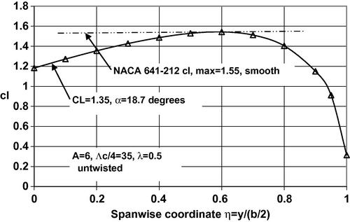
Figure 5.25 Spanwise distribution of the local lift coefficient for a swept wing with A = 6, Λ = 35°, and λ = 0.5, and no twist at an angle of attack α = 18.7°. Also shown is the maximum lift coefficient for the smooth NACA 641-212 airfoil section which is set normal to the quarter-chord line.
5.4.9 The pressure difference rule for CL,max
Panel methods for predicting the surface pressure over a real wing are described in Appendix C. Such computational methods provide a distribution of pressure, chordwise and spanwise, as detailed as the paneling used to approximate the wing’s surface. Valarezo and Chin (1994) use a panel method to develop the inviscid flow over a wing or wing body, with or without high lift devices, and then introduce an empirical relation for the airfoil characteristics to estimate the maximum lift of a wing. The method is based on the experimental observation that, under maximum lift conditions, the difference between Cp,peak, the peak suction pressure coefficient of an airfoil section of the wing, and Cp,t.e., the pressure coefficient at the trailing edge, is defined solely by the Mach number and Reynolds number of the flow over the airfoil and not the details of the airfoil’s shape. Because Valarezo and Chin (1994) are mainly interested in takeoff characteristics the Mach number range they deal with is limited to 0.15 < M < 0.25. They point out that Smith (1975) suggested two empirical criteria for defining the point at which the maximum lift is reached: first, the case where the upper surface velocity becomes sonic, Cp = Cp* and second, where M2Cp,peak = −1. The former suggestion, which for isentropic flow yields Cp = −13 at M = 0.223, has been often used as a rule of thumb for wings with no leading edge devices. The latter suggestion is based on data obtained at M > 0.4 and leads to negative pressure coefficients at low M which are below those observed in experiments.
The results of the method of Valarezo and Chin (1994), which they call the “pressure difference” rule, are shown to be quite accurate and its application has found a following in the airplane design community. The method is applied as follows:
1. Compute the flow field for the wing or wing-body combination using a panel method, assuring adequate definition of the flow at the leading and trailing edges, and plot the computed pressure difference Cp,peak − Cp,t.e. as a function of spanwise distance for several values of the wing lift coefficient.
2. Plot the absolute value pressure difference quantity Cp,peak – Cp,t.e. as a function of spanwise coordinate for the Mach number and Reynolds number based on local chord of interest. Curves representing their empirical results for the pressure difference Cp,peak – Cp,t.e. = f(M, Rec) are given in Figure 2 of their paper. Interestingly, 13 < (Cp,peak – Cp,t.e.) < 14 for Rec > 10 million.
3. The spanwise position at which the curve of step 2 is tangent to one of the curves of step 1 defines the maximum lift coefficient and the point along the span at which stall will likely be initiated.
Note that this method is very similar to the method suggested by Abbott and Von Doenhoff as discussed previously. Consider that the maximum section lift coefficient may be computed from the following equation involving Cp,l and Cp,u, the pressure coefficients on the lower and upper surfaces of the wing, respectively:
Valarezo and Chin (1994) show data that indicate the scaled pressure coefficient on the upper surface of the airfoil is essentially a unique function of the normalized distance along the chord and therefore the second integral in the equation above is simply a number. No data are shown for the scaled pressure coefficient on the lower surface, but making the assumption that it also exhibits similarity with respect to the normalized chord, we may expect that
![]()
The pressure difference may be written as
The scaled data presented by Valarezo and Chin (1994) indicate that, at maximum lift, the ratio of the pressure coefficient at the trailing edge to that at the suction peak is a number independent of Reynolds number so that
![]()
This result suggests that the use of the section maximum lift coefficient to aid in determining the maximum wing lift as suggested by Abbott and Von Doenhoff (1959) is analogous to the pressure difference rule introduced by Valarezo and Chin (1994) and should be acceptable for preliminary design work when panel method results are not available.
Valarezo and Chin (1994) carry out a panel method solution for the clean wing tested by Lovell (1977) which has A = 8.35, Λc/4 = 28°, and λ = 0.35. Using their pressure difference method they predict CL,max = 1.04 at α = 12° which agrees well with the wind tunnel data. The spanwise distribution of section lift coefficient for this wing, according to Diederich’s (1952) method described in Appendix C, is shown in Figure 5.26. The maximum section lift coefficient for stall as predicted by the DATCOM method of Section 5.4.6 is cl,max = 1.2. The airfoil used by Lovell is 10.6% thick (streamwise) and though the shape is specified no specific airfoil data are given, only wing data. This airfoil would be 12% thick normal to the quarter-chord, for which we may assume a range of 1.5 < cl,max,Λ=0 < 1.6. Applying simple sweep theory suggests that the airfoil cl,max is in the range of 1.17–1.25. Figure 5.26 shows that this range is consistent with a prediction of stall. Thus we may expect a reasonable prediction of CL,max using the simpler prediction methods if a more accurate panel method is unavailable.
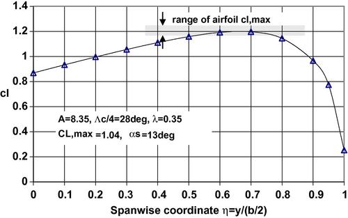
Figure 5.26 Spanwise distribution of the local lift coefficient for a swept wing with A = 8.35, Λc/4 = 28°, λ = 0.35, and no twist at an angle of attack α = 13°. Also shown is the estimated range of maximum lift coefficient for the smooth 10.6% thick (streamwise) RAE airfoil section used on the wing tested by Lovell (1977).
We may also examine the prediction of CL,max for this wing according to the simplified lifting line method presented previously in Section 5.4.7. Here Equation (5.30) yields CL/cl,max = 0.931. From Equations (5.32) and (5.33) we find KΛ1 = 0.0392 and KΛ2 = 0.658 so that Equation (5.31) yields KLΛ = 0.74. Because there is no twist KLΩ = 0 and therefore KLΩCL,αΩ/cl,max = 0. The airfoil normal to the quarter-chord line for this swept wing has been assumed to have 1.5 < cl,max < 1.6. Equation (5.34) yields a stall factor KLS = 0.967, resulting in a maximum lift coefficient from Equation (5.35) as follows:
![]()
Using the assumed values for cl,max yields 1 < CL,max < 1.067. The panel method result for this wing is CL,max = 1.04 at 13° angle of attack so that the simple modified lifting line technique yields a result about equivalent to that obtained with the pressure difference rule.
5.5 High lift devices
Airfoils that provide high lift to drag ratios necessary for efficient high-speed cruise are limited to values of cl,max < 1.4. As pointed out in Chapter 4, the operational values of CL for a wing in takeoff and landing are limited to values less than CL,max/1.44 to provide a stall margin for safety. Therefore, for an airfoil under takeoff or landing conditions the maximum cl achievable is cl ∼ 1. In takeoff, for example, the ratio of lift coefficient at takeoff to that at landing is given by
In Equation (5.36) we assumed that the wing loading in takeoff and at the start of cruise are approximately equal (W4/W3 = 0.98 from Table 2.3) and that takeoff occurs near sea level. For a typical cruise altitude around 33,000 ft (10 km) the atmospheric density ratio σ ∼ 1/3. Then with a typical cruise to takeoff velocity ratio Vcr/Vto ∼ 3, we find that CL,to/CL,cr ∼ 3. The lift coefficient in cruise is
The dynamic pressure under typical cruise conditions, where the atmospheric pressure ratio δ ∼ 1/4, is qcr ∼ pSL/10 ∼ 200 lb/ft2 (10 kPa). With typical wing loading values of around 125 lb/ft2 (6000 N/m2) we see that CL,cr ∼ 0.6. This result suggests that the takeoff value of lift coefficient is CL,to ∼ 1.8. Taking the stall margin safety factor into account shows that the maximum lift coefficient in takeoff required is CL,max,to ∼ 2.6, which is far more than an efficient high-speed airfoil can supply. As a consequence, some means must be found for enhancing the lift of an airfoil at low speed without affecting its aerodynamic efficiency at high speed. The most straightforward approach is to consider a variable geometry airfoil.
The lift is proportional to the circulation Γ that can be developed by the airfoil and this is primarily a function of turning the flow efficiently by means of a highly curved camber line. In order to generate the full circulation possible for a given airfoil the Kutta condition, i.e., the condition that the flow leaves the trailing edge of the airfoil smoothly, must be met. Separation of the low-momentum viscous boundary layer over the airfoil limits the degree to which this condition is satisfied. Thus, to achieve an effective high lift airfoil we must be able to increase the camber of the airfoil while simultaneously maintaining attachment of the boundary layer. A multi-element airfoil, comprised of movable elements, each of which is generating its own circulation and thereby contributing to an enhanced lift coefficient for the system, is the most cost-effective practical approach currently available.
Flow over airfoils with various types of moving elements in the vicinity of the trailing edge is illustrated in Figure 5.27 and those with various types of moving elements in the vicinity of the leading edge are shown in Figure 5.28. The airfoil elements are schematically indicated in these figures in order to emphasize the point that movable elements comprise the airfoil. These elements are stowed for high-speed flight so that the airfoil would appear as a straight line. Obviously, there are costs associated with the mechanisms required to deploy and stow the various elements shown. The tradeoff between airfoil performance and weight and cost penalties must be considered carefully.
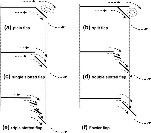
Figure 5.27 Schematic representation of typical trailing edge flap systems illustrating the nature of the flow guidance provided by the movable elements of each system.
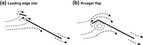
Figure 5.28 Schematic diagrams of two leading edge flap systems illustrating the nature of the flow guidance provided by the movable elements of each system.
The aerodynamic effects of the elements were described in detail by Smith (1975) and have been summarized by van Dam (2002) as follows:
1. The wake flow from an upstream element reduces the suction peak on the following element thereby reducing pressure recovery demands and delaying separation on that following element. This is called the slat effect.
2. Circulation produced by a downstream element increases the loading on the previous element, increasing its lift as well as increasing its pressure recovery demands. This is the circulation effect.
3. High-velocity flow on the upper surface of the downstream element permits the flow to leave the upstream element at higher speed, reducing the pressure recovery requirements on the forward element. This is the “dumping” effect.
4. Off-surface pressure recovery is more efficient than pressure recovery on a wall where pressure equilibrates less easily than in a free wake.
5. Fresh boundary layers appear on each element and the thinner boundary layers can withstand adverse pressure gradient better than thicker ones. Sufficient gap width ensures that the boundary layer grows independently on each element.
5.5.1 Airfoil with trailing edge flaps
The deployment of a trailing edge flap changes the camber of the airfoil and thereby increases the maximum lift coefficient and decreases the zero-lift angle of attack as depicted schematically in Figure 5.29.
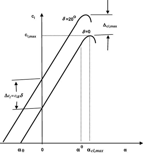
Figure 5.29 The generic change in the lift curve of an airfoil when a trailing edge flap is deflected.
A schematic diagram of a double-slotted flap was shown in Figure 5.27(d). The practical embodiment of such a flap on an airfoil is presented, for example, in Abbott and Von Doenhoff (1959) and is shown in Figure 5.30. The mechanism for driving the flap is not shown but the travel of the individual elements should be clear. In the stowed position, Figure 5.30(a), the airfoil shape is suitable for efficient high-speed flight. In the fully deployed position, Figure 5.30(b), the two slots separated by a small airfoil element are readily seen. Note that the travel of the flap is such that the projected elemental wing area dS is not materially changed. The increase in maximum lift coefficient for that airfoil is shown as a function of flap deflection angle in Figure 5.31. Though the maximum lift coefficient may be increased further by using triple-slotted flaps, such as those employed on the Boeing 737 shown in Figures 5.32 and 5.33, and on the Boeing 747, experience has shown that the added weight and complexity of such flaps are not completely cost-effective in airline operations. As a consequence, most trailing edge flap systems on jet transports are of the double-slotted type.
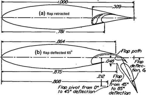
Figure 5.30 Airfoil with a double-slotted flap shown in the (a) retracted position and (b) fully deflected position, δf = 65°.
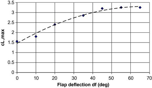
Figure 5.31 The maximum lift coefficient as a function of flap deflection for the double-slotted flap shown in Figure 5.20.
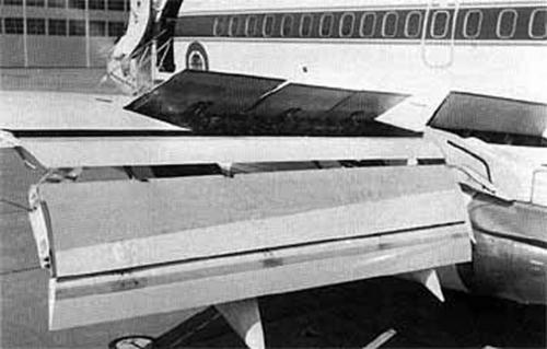
Figure 5.32 Upper-surface view showing triple-slotted flap and spoilers on Boeing 737 airplane [NASA].
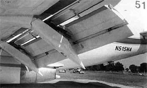
5.5.2 DATCOM method for trailing edge flaps
An empirical method for predicting airfoil maximum lift increments for plain, split, and slotted flaps is presented in DATCOM and will be followed here. The maximum lift increment provided to an airfoil by the deflection of a trailing edge flap is given by
Here (Δclmax)base is the section maximum lift increment for 25 percent-chord flaps at the reference flap-deflection angle and is shown in Figure 5.34 for different flap systems. The quantity k1 is a factor accounting for flap-chord-to-airfoil-chord ratios, cf/c, other than 0.25 and is shown in Figure 5.35. The quantity k2 is a factor accounting for flap deflections other than the reference value and is shown in Figure 5.36. Finally, k3 is a factor accounting for flap motion as a function of flap deflection and is shown in Figure 5.37. A sample calculation for the maximum lift increment for an airfoil with a trailing edge flap according to the DATCOM method is presented in the next section.
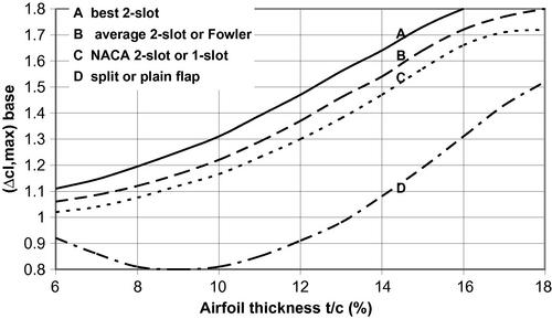
Figure 5.34 Base maximum lift increments for 25% chord trailing edge flaps of various types at the reference flap angle. Curve A is for best 2-slot flaps with NACA airfoils, B is for 2-slot flaps with NACA airfoils or Fowler flaps with any airfoil, C is for NACA 2-slot flaps with NACA 6-series airfoils or NACA 1-slot flaps with any airfoil, and D is for split and plain flaps with any airfoil.
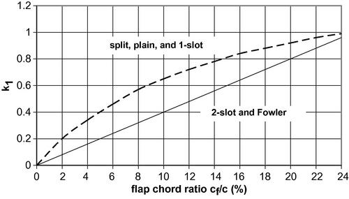
Figure 5.35 Correction factor for trailing edge flap chord to airfoil-chord ratios, cf/c, other than 0.25.
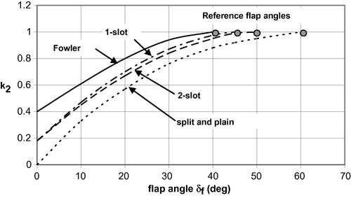
Figure 5.36 Flap angle correction factor. The reference flap angle for each type of flap is shown as a solid symbol at k2 = 1.
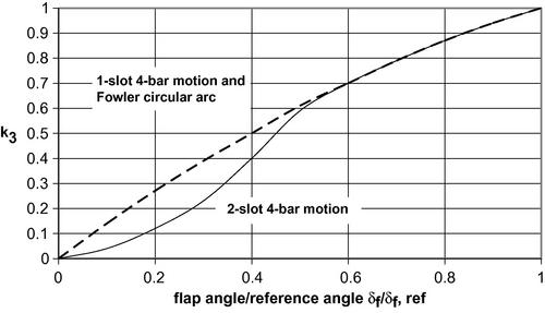
5.5.3 Sample calculation of airfoil with a trailing edge flap
Assume that one selects a smooth NACA 65-210 airfoil operating at a Reynolds number Rec = 6 × 10⁶. Consider the use of a double-slotted flap on this airfoil and a deflection through δf = 40°. The chord length of the flap is cf /c = 0.312. First it is necessary to compute (Δcl,max)base using Figure 5.34. Selecting an NACA double-slotted flap with the chosen NACA 6-series airfoil requires the use of curve C. The NACA 65-210 airfoil is 10% thick, as indicated by the last two digits in the airfoil designation, and entering this thickness on curve C in Figure 5.34 yields (Δcl,max)base = 1.165. The required flap chord ratio cf /c = 0.312 is off the scale shown in Figure 5.35 so the value of k1 must be extrapolated. For a double-slotted flap the k1 curve is linear and is given by k1 = 0.04(cf/c) where cf/c is in percent. Therefore the value of k1 = 1.25. Then k2 is found, from Figure 5.36 for a double-slotted flap at δf = 40°, to be k2 = 0.95. To find k3 the ratio of the actual flap angle selected to the reference flap angle, δf/δf,ref, for a double-slotted flap must be found. Following the curve for a double-slotted flap in Figure 5.36 up to k2 = 1 locates the flap reference angle as δf,ref = 50o. Then δf/δf,ref = 0.8 is entered in Figure 5.29 to find k3 = 0.87. Using Equation (5.37) we find the increment in cl,max for the airfoil to be
![]()
This result is about 10% less than the experimental value reported by Cahill (1947).
We may also consider the trailing edge flap for a wing in the takeoff configuration where the flap deflection is much smaller than the maximum, δf = 15.6°. The wing has an aspect ratio A = 5.1, a taper ratio λ = 0.383, and a quarter-chord sweep angle Λc/4 = 46°. The wing uses an NACA 64-210 airfoil normal to the leading edge with a resulting thickness to chord ratio t/c = 0.072 in the streamwise direction. The wing has a single-slotted flap with a flap to airfoil-chord ratio cf/c = 0.258 with a rated area Sf/S = 0.378 and the Reynolds number based on chord Re,c = 6.0 × 10⁶. We first use Figure 5.34 to find (Δcl,max)base = 1.045, then enter Figure 5.35 to find k1 = 1.010. Figure 5.36 yields k2 = 0.605 and we calculate (flap angle)/(reference flap angle) = 15.6/45 = 0.347. Figure 5.37 provides k3 = 0.445. We may compute the section maximum lift coefficient from Equation (5.37) as follows:
![]()
The sweepback correction KΛ = 0.730 and therefore the total maximum lift coefficient is
![]()
This result is of course based on the reference wing planform area S and compares well with a laboratory test value of 0.075.
5.5.4 Airfoil with leading edge slats or flaps
A method has been developed for predicting the stall of comparatively thin airfoils with leading edge flaps or slats. Modern airliners generally are equipped with slats since they are relatively simple and provide lift augmentation with little drag penalty. A schematic illustration of the operation of a typical leading edge slat appears in Figure 5.38. The change in the lift curve produced by the addition of a leading edge slat is shown in Figure 5.39. Leading edge slat installations on a Boeing 737 and an Airbus A310 are shown in Figures 5.40 and 5.41, respectively. Leading edge flaps in use on commercial transport are Krueger flaps (see, for example Torenbeek, 1982) and the approach presented is not applicable to them. The DATCOM estimation method, which is presented here, is based on the assumption that the flapped and unflapped airfoils stall when the respective pressure distributions about the noses are the same. The method gives best results for slat deflections less than 20° and slat-chord-to-airfoil-chord ratios less than 0.20.
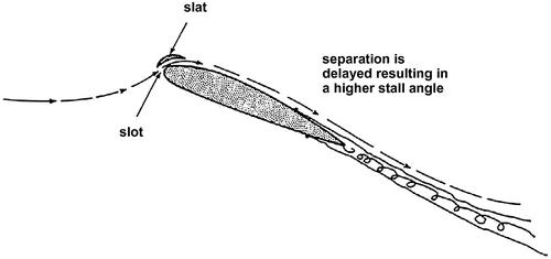
Figure 5.38 Lift on the leading edge slat increases lift while the flow over it energizes the boundary layer over the main airfoil delaying separation.
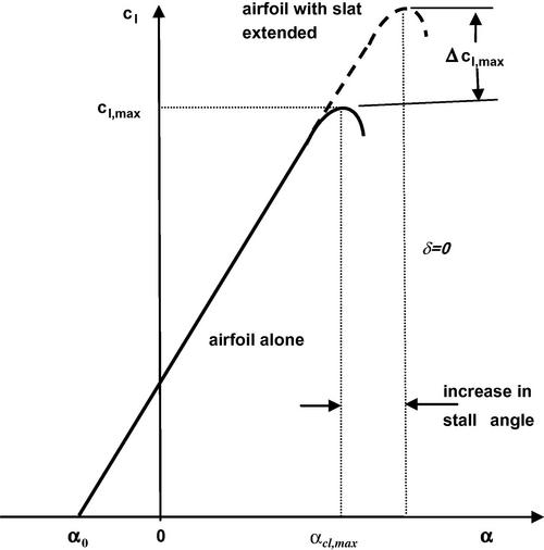
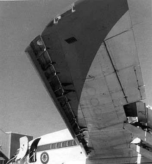
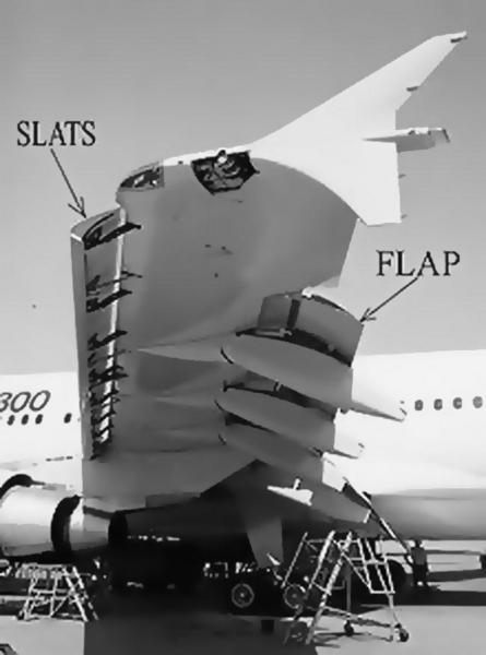
Figure 5.41 Leading edge slats and trailing edge flaps on Airbus A310-300. The fairings for the trailing edge flap drive mechanisms are in the deflected position.
Leading edge flaps are of two types: a drooping leading edge, which is a simple flap hinged downstream of the leading edge, and an extensible leading edge that basically increases the chord. The former is complicated in application and, though well studied, has found application only on the furthest inboard station on the Airbus A380 and not on any other operating commercial jet transports. One type of leading edge flap is the Krueger flap whose simplicity makes it a commonly used leading edge high lift device. Several manifestations are schematically illustrated in Figure 5.42.
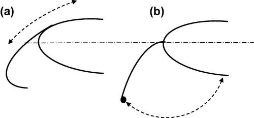
The feature differentiating leading edge flaps from slats is that the former have their trailing portions coincident with the airfoil surface so that there is no slot formed as there is in a leading edge slat system. These simple embodiments of a leading edge flap may be made more elaborate by having a position which produces a slot, thereby emulating a slat. This variation culminates in the highly developed variable camber Krueger (VCK) flap used by Boeing. In the VCK flap a linkage system permits the flap to be extended and cambered in various configurations in order to achieve optimal lift production in several flap settings.
5.5.5 DATCOM method for leading edge slats and flaps
Though leading edge flaps, that is, hinged nose sections on airfoils, have been the subject of much study they are not used on any commercial aircraft. The leading edge slat is the most common leading edge device in wide use. The leading edge slat is analogous to the slotted trailing edge flap in that the slat and the remainder of the airfoil form a two-element airfoil with all the advantages described at the beginning of this section. As explained previously, the leading edge slat increases the maximum lift coefficient of the airfoil along with the stall angle. As a result, they are commonly used, particularly in landing, though they are also useful on takeoff because the lift increment they develop comes with little drag penalty.
The DATCOM method for leading edge flaps and slats proposes that the maximum lift increment for leading edge flaps or slats may be approximated by the following empirical relation:
The first term in Equation (5.38) is the theoretical lift effectiveness which gives the rate of change of the lift coefficient with change in deflection angle; it is shown in Figure 5.43 as a function of the leading edge flap or slat chord to airfoil-chord ratio cs/c. The second term in Equation (5.38), ηmax, is an empirical factor which accounts for the effects of airfoil leading edge radius and maximum thickness. A graph of this factor is presented in Figure 5.44; the discontinuity in the curve for slats is said to be due to a lack of data in the region of the discontinuity. An ad hoc correction is proposed there which provides more accurate results as will be shown in the sample problems to follow.
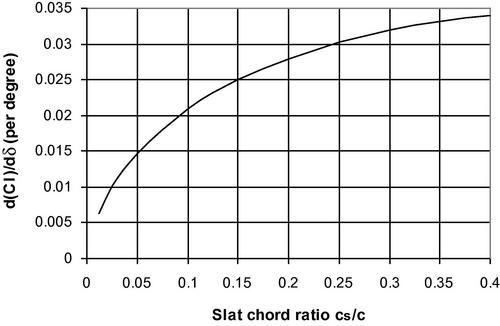
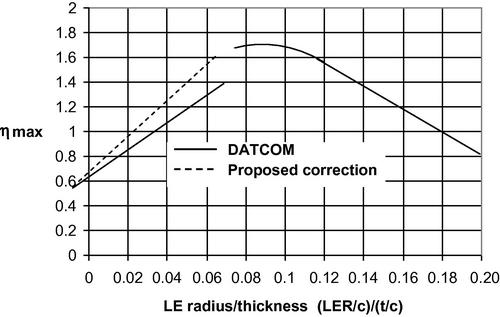
The third term, ηδ, is another empirical factor which corrects for flap or slat deflections different from the optimum flap angle. This parameter is shown in Figure 5.45 as a function of the flap or slot deflection angle δs. The deflection angle is defined in Figure 5.46. To understand the angle δs one may first imagine drawing a chord line on the slat-airfoil combination when the slat is stowed. Then when the slat is deflected, the segment of the chord line that was drawn on the slat in the stowed position has now rotated through the deflection angle δs. This is the standard used in the DATCOM method and is not necessarily used throughout the literature as a definition of slat deflection angle. The ratio c’/c accounts for the apparent increase in chord length when the slat is deflected and a slot is formed between the two airfoil elements; these dimensions are illustrated in Figure 5.46.
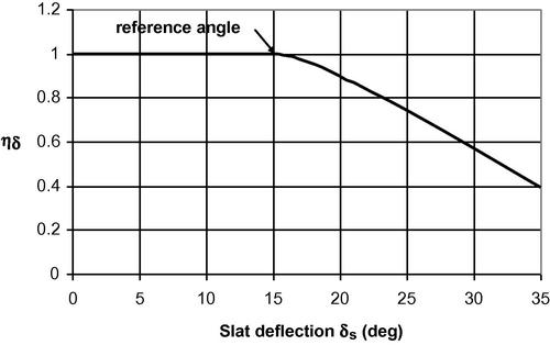
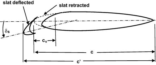
5.5.6 Sample calculations of airfoil with a leading edge slat
Consider a smooth NACA 64A010 airfoil operating at a Reynolds number Rec = 6 × 10⁶. The NACA 64-series airfoil has a leading edge radius of 0.72% chord, according to Table 5.3. However, the letter A in the airfoil designation denotes a modified thickness distribution and experiments performed by Hayter and Kelly (1953) indicate a leading edge radius LER = 0.687% chord. The airfoil is 10% thick, the slat deflection δs = 25.6°, the slat chord to airfoil-chord ratio is cs/c = 0.17, and the ratio c’/c = 1. From Figure 5.43 we estimate ![]() = 0.026 and from Figure 5.44 we enter (LER/c)/(t/c) = 0.687%/10% = 0.0687 and find ηmax = 1.32. Entering Figure 5.45 with δs = 25.6° yields ηδ = 0.75. Then
= 0.026 and from Figure 5.44 we enter (LER/c)/(t/c) = 0.687%/10% = 0.0687 and find ηmax = 1.32. Entering Figure 5.45 with δs = 25.6° yields ηδ = 0.75. Then
This result obtained is conservative, about 15% less than the result of 0.84 reported by Hayter and Kelly (1953). However, using the proposed correction in Figure 5.44 leads to ηmax = 1.59 which changes the answer for the maximum lift increment to Δcl,max = 0.855 which is now 1.8% larger than the measured value.
Gottlieb (1949) studied the effect of leading edge slats on two smooth airfoils: a NACA 641-212 airfoil and a NACA 65A109 airfoil, both operating at a Reynolds number based on airfoil-chord Rec = 6 × 10⁶. The NACA 64-series airfoil has a leading edge radius of 0.72% chord, according to Table 5.3. The airfoil is 12% thick, the slat deflection δs = 14.3°, the slat chord to airfoil-chord ratio cs/c = 0.14, and the ratio c’/c = 1.1. From Figure 5.43 we estimate ![]() = 0.024 per degree and from Figure 5.44 we enter (LER/c)/(t/c) = 0.72%/12% = 0.06 and find ηmax = 1.2. Entering Figure 5.45 with δs = 14.3° yields ηδ = 1. Then
= 0.024 per degree and from Figure 5.44 we enter (LER/c)/(t/c) = 0.72%/12% = 0.06 and find ηmax = 1.2. Entering Figure 5.45 with δs = 14.3° yields ηδ = 1. Then
This result obtained is quite conservative, 25% less than the result of 0.6 reported by Gottlieb (1949). However, using the proposed correction in Figure 5.44 we obtain ηmax = 1.47 and the new result for the lift increment is Δcl,max = 0.55 which is about 8% smaller than the reported value. The 65A109 airfoil is 9% thick, the slat deflection δs = 24.3°, the slat chord to airfoil-chord ratio cs/c = 0.14, and the ratio c’/c = 1.09. From Figure 5.43 we estimate ![]() = 0.024 per degree and from Figure 5.44 we enter (LER/c)/(t/c) = 0.55%/9% = 0.061 and find ηmax = 1.22. Entering Figure 5.45 with δs = 24.3o yields ηδ = 0.76. Then
= 0.024 per degree and from Figure 5.44 we enter (LER/c)/(t/c) = 0.55%/9% = 0.061 and find ηmax = 1.22. Entering Figure 5.45 with δs = 24.3o yields ηδ = 0.76. Then
This result obtained is also conservative, about 15% less than the result of 0.69 reported by Gottlieb (1949). However, using the proposed correction in Figure 5.44 we obtain ηmax = 1.47 and the new result for the lift increment is Δcl,max = 0.71 which is about 3% larger than the reported value.
5.5.7 Combining leading and trailing edge devices on airfoils
Leading and trailing edge high lift devices have been shown to provide improved lifting performance over that possible with the airfoil alone. It follows that using them in combination should lead to better performance than that achievable with either leading edge or trailing edge devices alone. Two-dimensional experimental results for an NACA 64A010 airfoil section equipped with various combinations of a leading edge slat, leading edge flap, split flap, and double-slotted flap, were reported by Hayter and Kelly (1953). Wind tunnel experiments were performed at M = 0.18, and Rec from 2 million to 7 million with and without leading and trailing edge devices. The maximum lift coefficients obtained for these tests are shown in Figure 5.47.
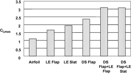
Figure 5.47 Maximum lift coefficients for an NACA 64A010 airfoil alone and with a leading edge flap (LE Flap), a leading edge slat (LE Slat), a double-slotted flap (DS Flap), a combination of double-slotted flap and leading edge flap (DS Flap + LE Flap), and a combination of double-slotted flap and leading edge slat (DS Flap + LE Slat).
The effect of the high lift devices on the angle of attack for maximum lift coefficient was also presented by Hayter and Kelly (1953) and is illustrated in Figure 5.48. When used alone, the leading edge devices dramatically increase the angle of attack capability of the airfoil. However, the angle of attack for maximum lift coefficient when the double-slotted flap is used alone is equally dramatically decreased from that for the airfoil alone. The use of either leading edge device in conjunction with the double-slotted flaps nearly restores the original angle of attack capability of the airfoil.
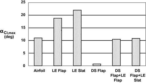
Figure 5.48 Angle of attack for the maximum lift coefficients for an NACA 64A010 airfoil alone and with a leading edge flap (LE Flap), a leading edge slat (LE Slat), a double-slotted flap (DS Flap), a combination of double-slotted flap and leading edge flap (DS Flap + LE Flap), and a combination of double-slotted flap and leading edge slat (DS Flap + LE Slat).
Using the results presented in Figure 5.47 we may show that the maximum lift coefficient for the combination of trailing and leading edge devices is approximately equal to the sum of the airfoil contribution, the leading edge device increment, and the trailing edge flap increment. In other words, the contribution of the high lift devices was additive. This result for an airfoil is shown in Figure 5.49. It must be noted that the results reported were for optimal positions and configuration of the high lift devices.
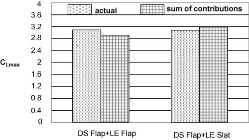
Figure 5.49 Measured maximum lift coefficients for an NACA 64A010 airfoil with a combination of double-slotted flap and leading edge flap (DS Flap + LE Flap) and a combination of double-slotted flap and leading edge slat (DS Flap + LE Slat) showing measured values as well as those obtained by summing the contributions of each component.
5.6 Determination of CL,max for the wing in takeoff and landing configurations
The DATCOM method for estimating the increment of ΔCLmax for the wing with flaps and slats deflected is used here. These devices have different drag penalties associated with their operation and each will be addressed in Chapter 7. A compilation of leading and trailing edge devices currently in use is presented in Table 5.6(b). The information included is drawn largely from Rudolph (1996) and manufacturers’ literature, among other sources.
High Lift Systems on Commercial Jet Transports
| Airplane | Trailing Edge Devices | Leading Edge Devices |
| B707 | Fixed vane/main double-slotted | Simple Krueger |
| B727 | Triple-slotted | 3-position slats, Inboard FBNK |
| B737 | Triple-slotted | 3-position slats, Inboard FBNK |
| B747 | Triple-slotted | VC Krueger |
| B757 | Main/aft double-slotted | 3-position slats |
| B767 | Main/aft double-slotted inboard, | 3-position slats |
| Single-slotted outboard | ||
| Drooped inboard aileron | ||
| B777 | Main/aft double-slotted inboard | 3-position slats, |
| Single-slotted outboard | ||
| Drooped and slotted inboard aileron | ||
| B787-8 | Single-slotted in- and outboard | 3 position slats, Inboard S/S Krueger |
| Flaperon with droop function | ||
| DC-8 | Fixed vane/main double-slotted | 3-position slats |
| DC-9-10 | Fixed vane/main double-slotted | none |
| DC-9-30/50 | Fixed vane/main double-slotted | 3-position slats |
| DC-10 | Articulating vane/main double-slotted | 3-position slats |
| MD-80 | Fixed vane/main double-slotted | 3-position slats |
| MD-11 | Articulating vane/main double-slotted | 3-position slats |
| Drooped inboard aileron | ||
| A300B | Main/aft double-slotted | 3-position slats, Inboard FBNK |
| A300-600 | Single-slotted | 3-position slats, Inboard FBNK |
| Drooped inboard aileron | ||
| A310 | Articulating vane/main inboard, | 3-position slats |
| Single-slotted outboard | ||
| Drooped inboard aileron | ||
| A320 | Single-slotted | 3-position slats |
| A321 | Main/aft double-slotted | 3-position slats |
| A330 | Single-slotted | 3-position slats |
| Drooped outboard aileron | ||
| A340 | Single-slotted | 3-position slats |
| Drooped outboard aileron | ||
| A380 | Trailing edge flaps | Inboard slat and drooped nose |
| Outboard short chord slats | ||
| Fuselage side fixed leading edge |
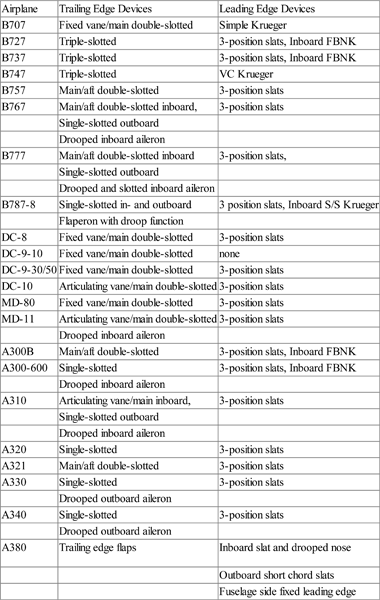
Notes: FBNK = folding, bull-nose Krueger, S/S Krueger = slat and seal Krueger.
5.6.1 Application of high lift devices on wings
We have discussed the determination of the lift of a three-dimensional wing in Section 5.4. The discussion of leading and trailing edge high lift devices has thus far been confined to airfoils, that is, two-dimensional wings. However, Furlong and McHugh (1953) point out and Hoak et al. (1978) repeat that the lift increments due to leading and trailing edge devices are not, in general, additive. When both are deployed the resulting lift increment is not necessarily the sum of the lift increments produced by each when working alone. To appreciate this fact we turn to the early experimental work compiled by Furlong and McHugh (1953) which illustrates some of the features of leading and trailing edge high lift devices used independently and in concert on three-dimensional swept wings.
One wing considered by Furlong and McHugh (1953) is reasonably typical of commercial jet transports, having an aspect ratio A = 6, quarter-chord sweep Λc/4 = 35o, and taper ratio λ = 0.5. A sketch of the wing is shown in Figure 5.50. Wind tunnel experiments were performed at M = 0.18, and Rec = 9.35 × 10⁶ with and without leading and trailing edge devices. The wing was constructed using the NACA 641-212 airfoil aligned with the free stream direction.
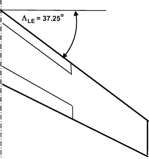
Figure 5.50 Planform of a wing with an NACA 641-212 airfoil, A = 6, ΛLE = 37.25o, and λ = 0.5 showing leading and trailing edge high lift devices.
We compare the performance of the airfoil to that of each high lift device alone and then to that of a combination of both leading and trailing edge devices for the case in which high lift devices have a spanwise extent of 50%. The leading edge devices include a flap or a slat, while the trailing edge device is a double-slotted flap. The maximum lift coefficient achieved by the wing of Figure 5.50 using various combinations of high lift devices is shown in Figure 5.51. It is seen that the two leading edge devices give about the same increment in maximum lift coefficient over that produced by the airfoil alone—about a 10% improvement. The double-slotted flap alone provides a 50% improvement over the airfoil alone. However, when either of the leading edge devices is used in conjunction with the double-slotted flap there is essentially no change, or even a slight decrease in maximum lift coefficient. At the same time, it is also shown in Figure 5.51 that if the spanwise extent of the leading edge flap is increased to 65% the use of both the leading edge flap and the (50% span) double-slotted flaps leads to an improvement over that with the flap alone. The extent to which the notion of the effects of each high lift coefficient contribution being additive is illustrated in Figure 5.52.
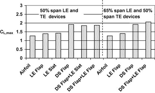
Figure 5.51 Maximum lift coefficients for the wing of Figure 5.38 with different combinations of high lift devices. The notation is as follows: NACA 641-212 airfoil alone and with a leading edge flap (LE Flap), a leading edge slat (LE Slat), a double-slotted flap (DS Flap), a combination of double-slotted flap and leading edge flap (DS Flap + LE Flap), and a combination of double-slotted flap and leading edge slat (DS Flap + LE Slat).
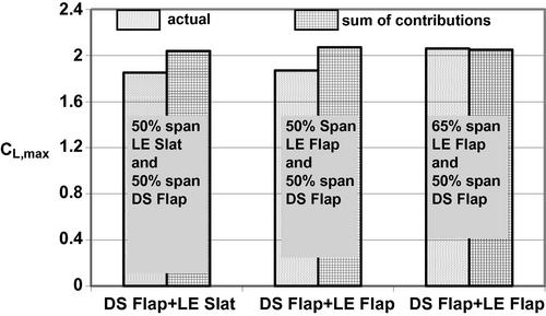
Figure 5.52 Comparison of measured CL,max for the wing of Figure 5.38 with different combinations of high lift devices with the result of simply summing the individual contributions for each component. Notation is as given in Figure 5.39.
Here we see that the increase in spanwise extent of the leading edge flap to 65% from 50% resulted in a situation where the sum of the individual contributions of the high lift devices gives a good approximation to the actual value for the components in combination.
It must be noted that the results discussed in some detail here are intended to demonstrate that the effects of leading and trailing edges on wing performance are not necessarily additive. However, the widespread use of these devices in commercial jet transports indicates that better combined performance can be achieved than this set of wind tunnel experiments might suggest. To achieve synergetic performance between the leading and trailing edge devices careful attention must be paid to the integration of these elements, as explained by Smith (1975). Reasons beyond lift performance alone help explain the widespread use of combined leading and trailing edge high lift devices. An illustration of the implementation of elaborate high lift systems in practice is shown in Figure 5.53. There a Boeing 747-400 is depicted in the landing configuration. The triple-slotted trailing edge flaps and the variable camber Krueger flaps on the leading edges are clearly visible. The inboard Krueger flaps seal to the upper surface while the outboard ones have a clearly visible slot.
Figure 5.53 A Boeing 747-400 in the landing configuration showing the triple-slotted trailing edge flaps and the variable camber Krueger flaps on the leading edges. The inboard Krueger flaps seal to the upper surface while the outboard ones have a clearly visible slot and therefore act as slats.
Leading edge devices may be safely deployed at higher speeds than can the trailing edge flaps. Thus, in operations during the final stages of descent, where flight speeds are much lower than in cruise but substantially higher than in landing, leading edge flaps or slats may be extended to improve the lifting capability of the wing without incurring very large drag penalties. Besides a lift coefficient increase, using the leading edge flap or slot alone also produces a smaller pitch-up moment than does a trailing edge flap alone. This improves the handling qualities and reduces trim requirements. It is clear from Figure 5.48 that the use of a leading edge device alone increases the angle of attack for maximum lift coefficient while a trailing edge flap reduces it. Properly combining the use of leading and trailing edge high lift devices provides the benefit of increased lift at higher angles of attack than can be achieved using just the trailing edge flap alone. This is important in avoiding a tail strike, a situation where there is a rotation of the aircraft beyond the tail cone flare angle θTC, as shown in Figure 5.54. The higher maximum lift coefficients possible with a combination of leading and trailing edge devices generally result in reduced pitching-moment variation with angle of attack. This essentially neutral longitudinal motion response of the wing during terminal operations improves handling properties and reduces trim requirements. The fact that leading edge systems are relatively simple and easy to maintain means that the incremental cost of providing them is usually low enough to be attractive.
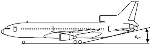
5.6.2 Determination of ΔCL,max for the wing due to flaps
The increment in maximum lift coefficient for the wing due to the trailing edge flap deflection is given in the DATCOM method by the following equation:
Here Δcl,max is the increment in lift coefficient due to flap deflection as defined in Equation (5.37). The quantity SW,f /S is the ratio of wing area affected by the trailing edge flap deflection (including both port and starboard wings) to the total wing area, as shown in Figure 5.55. The wing area affected by the flap may be written as
In Equation (5.39) the quantity λ = ct /cr is the taper ratio, i.e., the ratio of the tip chord to the root chord, and b is the wingspan. The non-dimensional inboard location of a flap is ηi = yi/(b/2), while the outboard location is ηo = yo/(b/2). If the flaps do not extend continuously along the trailing edge, as is the case in Figure 5.55, then the affected area for each may be calculated independently and added together. The wing planform area S is given by Equations (5.5) and (5.12) for straight-tapered wings and cranked wings, respectively. The correction factor for sweepback is
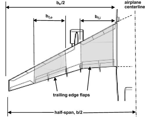
Figure 5.55 Plan view of wing where shaded area, including both the starboard and port wing, is the rated area for the flaps, that is, the portion of the wing planform area affected by the flaps.
It should be noted that the flap deflection angles and all dimensions are measured in planes parallel or perpendicular to the plane of symmetry. Then the lift coefficient for the wing with flaps deflected is
5.6.3 Determination of ΔCL,max for the wing due to slats
For preliminary design purposes the contribution to the maximum lift coefficient of the wing due to leading edge slat deflection, we assume an approach based on that used in estimating the contribution of the trailing edge flap and on the approach presented previously in Section 5.5.5. Then, in analogy with Equation (5.39), the airfoil results are extended to the wing as given by
The definitions of Equations (5.39), (5.40) and (5.41) hold, where now Sw,s is interpreted in terms of the wing area affected by the operation of the slat or flap, as depicted in Figure 5.56. Then the maximum lift coefficient of the wing with a leading edge slat deflection is
Because the careful integration of leading and trailing edge devices can lead to increments in maximum lift coefficient greater than either one alone we will assume that the estimates of Equations (5.39) and (5.43) may be added so that the combined lift coefficient for the wing is
At least two values of the total maximum lift coefficient of the wing CL,max,w should be calculated; one for takeoff and the other for landing.
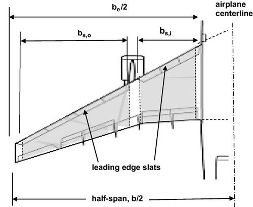
Figure 5.56 Plan view of wing where shaded area, including both the starboard and port wing, is the rated area for the slats, that is, the portion of the wing planform area affected by the slats.
5.6.4 Sample calculation for flaps and slats
Consider the wing investigated by Koven and Graham (1948) and illustrated in Figures 5.57 and 5.58. The wing has an aspect ratio A = 6, a taper ratio λ = 0.5, and a leading edge sweep angle Λc/4 = 37.25°. The wing uses an NACA 641-212 airfoil normal to the free stream with a thickness to chord ratio t/c = 0.098 in the streamwise direction. The wing has a double-slotted flap with a flap to airfoil-chord ratio cf/c = 0.25 and the rated area may be calculated to be Sw,f/S = 0.951 for the full-span flap and 0.573 for the half-span flap. The Reynolds number based on chord Re,c = 6.0 × 10⁶ and the full flap deflection is δf = 48.85°.
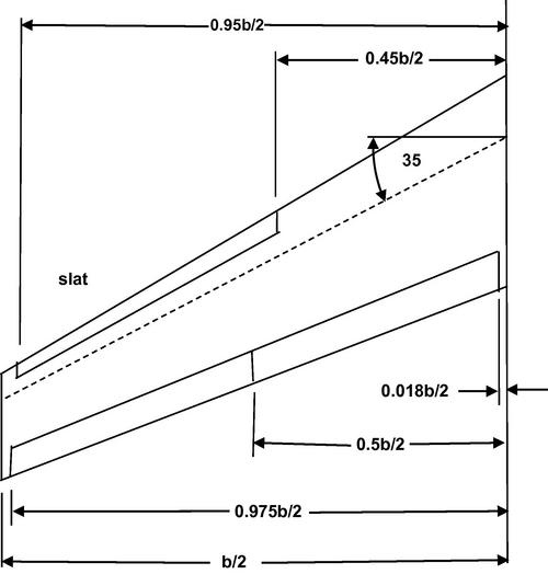
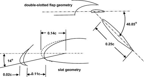
Figure 5.58 Details of high lift devices for the wing in Figure 5.46.
We first use Figure 5.34 to find (Δcl,max)base = 1.31, then enter Figure 5.35 to find k1 = 1. Figure 5.36 yields k2 ∼ 1 and for the flap angle of 48.85°Figure 5.37 provides k3 = 1. We may compute the section maximum lift coefficient from Equation (5.37) as follows:
![]()
The quarter-chord sweepback angle is Λc/4 = 35.17° and the sweepback correction KΛ = 0.815 and therefore the total maximum lift coefficient is
![]()
The wing maximum lift coefficient with no high lift devices deployed is 1.27 so that with the full-span flaps employed the maximum lift coefficient becomes
![]()
The experimental value with full-span flaps is CL,max = 2.32 so the error is −1.5%. For the case of half-span flaps the increment in maximum lift coefficient is
![]()
The wing maximum lift coefficient with no high lift devices is 1.27 so that with the half-span flaps deployed the maximum lift coefficient becomes
![]()
The experimental value with full-span flaps is CL,max = 1.92 so the error is −2%.
The wing also has slats and the rated area may be calculated to be Sw,s/S = 0.42. The nose flap to chord ratio is 0.14 and from Figure 5.43 we find ![]() . From Table 5.3 the leading edge radius LER = 1.04% chord so that the ratio (LER/c)/(t/c) for this airfoil is 0.087 and from the curve in Figure 5.36 ηmax = 1.7. For 14° deflection Figure 5.37 suggests ηδ = 1 and from Figure 5.47 we calculate c’/c = 1.11. Using these values in Equation (5.38) yields
. From Table 5.3 the leading edge radius LER = 1.04% chord so that the ratio (LER/c)/(t/c) for this airfoil is 0.087 and from the curve in Figure 5.36 ηmax = 1.7. For 14° deflection Figure 5.37 suggests ηδ = 1 and from Figure 5.47 we calculate c’/c = 1.11. Using these values in Equation (5.38) yields

Then the increment in maximum lift for the wing with slats deployed is
![]()
The wing maximum lift coefficient with no high lift devices is 1.27 so that with the half-span slats deployed the maximum lift coefficient becomes
![]()
The experimental value with half-span slats is CL,max = 1.42 so the error is +4.9%.
Although the estimates presented are quite accurate for the flaps alone or the slats alone, the same is not true if the increments for half-span flaps and half-span slats are simply added. In that case the maximum lift coefficient for the wing would be
![]()
The experimental value for this case is reported as CL,max = 1.85, an error of +13.5%. Indeed, the experimental value for the maximum lift coefficient with only the half-span flaps deployed is better than that observed with both flaps and slats deployed. The slats had little effect on maximum lift coefficient or maximum angle of attack when used in combination with the flaps. It was also observed, as expected, that the use of the slats alone increased the maximum angle of attack from 19° for the airfoil alone to 26°, while the use of the half-span flaps decreased the maximum angle of attack to 14.3°. However, when both are deployed the maximum angle of attack remains the same as with the flaps alone. This provides another demonstration that the incorporation of both leading and trailing edge high lift devices on a wing must be carried out carefully because the effects of each are not necessarily additive.
5.7 Development and layout of the preliminary wing design
The weight of the aircraft at all stages of the mission, as well as the selected cruise Mach number and altitude, is known from the results in Chapter 2. The fuselage dimensions, including the length lf, the diameter df, and the tail cone flare angle θTC, were determined in Chapter 3. The required wing area S, along with the estimated values of lift coefficient in takeoff and landing is known from the results of Chapter 4. Using this information and the methods presented in the current chapter a preliminary layout of the wing design may be carried out.
5.7.1 Aspect ratio
The jet transport database suggests that there is no reliable simple correlation between the aspect ratio and previously calculated characteristics of the proposed aircraft. For example, consider the relationship between the aspect ratio A and the takeoff weight Wto for 49 commercial turbofan and turboprop transport aircraft as shown in Figure 5.59. There is no clear correlation, but it is apparent that turboprops with unswept wings employ the highest values of A. Turbofan-powered swept wing aircraft with fewer than 200 passengers (Np < 200) show a clear upward trend from A = 8 to A = 10, while turbofans with Np > 200 cover a much broader range of the design space, but with a somewhat downward trend as the takeoff weight grows.
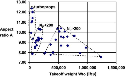
Figure 5.59 Variation of the aspect ratio with takeoff weight for 49 commercial turbofan and turboprop transport aircraft with different passenger loads Np.
As another example, we may consider the variation of aspect ratio as a function of a combined variable which is also known for the design aircraft, the takeoff wing loading (W/S)to, as shown in Figure 5.60. Again, there are no clear-cut trends although the turboprops and turbofans are more clearly separated. The turbofan-powered aircraft show an upward trend in aspect ratio as the wing loading increases, but the range 7.5 < A < 10.5 is covered in the wing loading range 100 lb/ft2<(W/S)to < 150 lb/ft2. Thus, the choice of aspect ratio is well bounded, but without a straightforward means of choosing a value. However, the span loading (W/b2)to of the aircraft in the database, which is shown as a function of takeoff weight in Figure 5.61, shows a rather unusual trend. This parameter is related to induced drag and one may use this figure to determine a reasonable span loading from which an estimate may be made of the span of the design aircraft. From that result and the known wing area a provisional aspect ratio A = b2/S may be determined. The result of this approach for selecting an initial value of aspect ratio should be weighed in light of the market survey aircraft values and modified accordingly, if necessary.
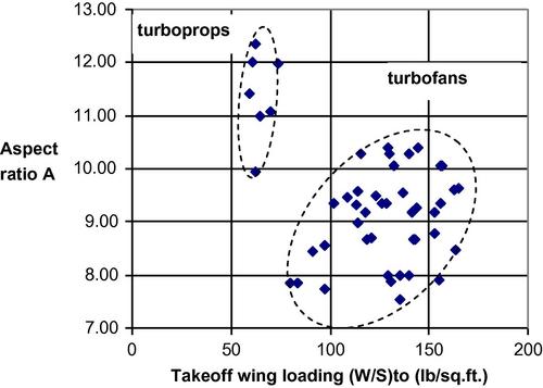
Figure 5.60 Variation of the aspect ratio with takeoff wing loading for 49 commercial turbofan and turboprop transport aircraft.
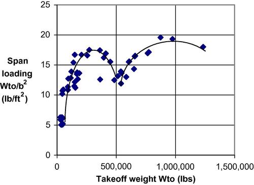
Figure 5.61 Span loading as a function of takeoff weight for 49 commercial turbofan and turboprop transport aircraft. Faired curve is added to aid in depicting trends.
5.7.2 Taper ratio and the root chord
Assuming a straight leading edge, Equation (5.5) may be used to determine the root chord cr once a taper ratio λ is selected. De Young and Harper (1948) provide a theoretical estimate for the variation of the taper ratio as a function of quarter-chord sweep angle for wings with an approximately elliptic span loading independent of aspect ratio, and this is shown as a curve in Figure 5.62. Also shown on that plot is the region occupied by current jet transport configurations. As one moves to the right of the curve in Figure 5.62 the loading moves outboard as the aspect ratio increases.
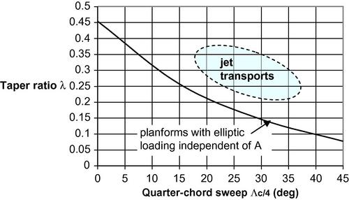
Figure 5.62 Variation of the taper ratio with quarter-chord sweep angle for wings with an approximately elliptic span loading. The shaded region contains values typical of current jet transports.
The taper ratio may be selected using the market survey values as a guide, which will generally show 0.25 < λ < 0.35. Then the tip chord ct is determined from the definition of the taper ratio, λ = ct/cr. The wing sweepback angle remains to be selected and this may be varied while keeping constant all other parameters chosen thus far. This is shown in Figure 5.63 for a wing with aspect ratio A = 7 and taper ratio λ = 0.33 but two different leading edge sweep angles, 25° and 35°, which are typical for jet transports. It should be clear from Figure 5.56 that the larger the sweepback, the larger the cantilever length of the 50% chord line sc/2,Λ = b(2cosΛc/2). This suggests that wing root bending moment that must be resisted by the structure will also grow with increasing sweepback.
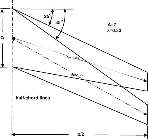
Figure 5.63 The length of the locus of half-chord points along a wing of constant A and λ for different leading edge sweepback angles.
Here the thickness of the root chord tr resists the bending moment caused by the lift distribution of the wing. Consider the simple case of the bending stress in a cantilever beam of length sc/2 = b/(2cosΛc/2) and hollow rectangular cross-section with width cr, depth tr, and uniform thickness t. If the half-span wing lift acts at the spanwise center of pressure location yc.p., and equals half the aircraft weight W, then the bending stress is given by
We may normalize the bending stress by the ratio of supported weight to approximate structural cross-sectional area as follows:
Thus we see that b/(2trcosΛc/2) logically appears as a basic structural parameter for the wing design. Indeed, Torenbeek (1982) shows data indicating that for jet transports, over a wide range of weights, the parameter
Now, with a good estimate for the root thickness ratio we can identify an equally reasonable value for the wing sweepback. We realize that for a given value of A and λ, a lower sweepback permits a thinner wing and this would save wing weight. On the other hand, a greater sweepback reduces the component of Mach number normal to the leading edge, Mn = McosΛLE, and this reduces compressibility drag. Striking an appropriate balance between conflicting requirements such as this is typical of the tradeoffs surfacing in all aspects of airplane design.
5.7.3 Wing relative thickness and airfoil selection
With the planform of the wing determined it is necessary to select an airfoil with appropriate shape and thickness appropriate to the cruise Mach number Mcr, cruise altitude zcr, and sweep angle Λc/4 that have already been selected. Scholz and Ciornei (2005) reviewed and evaluated a dozen theoretical and empirical approaches for estimating the thickness to chord ratio of a commercial jet transport wing at high subsonic speeds in terms of M, Λc/4, CL, and airfoil type. They compared the results obtained for all approaches with the measured relative thickness for 29 jet transport wings using the following definition for relative thickness suggested by Jenkinson, Simpkin, and Rhodes (1999):
Scholz and Ciornei (2005) found that the two most accurate results were obtained by regression analysis and by the theoretical approach proposed by Torenbeek (1982). Inasmuch as the regression equation is more readily implemented it is used here in the form
Here ka = 0.921 for conventional airfoils, 0.928 for peaky airfoils, 0.932 for modern supercritical airfoils, and 1.012 for older supercritical airfoils. The quantity MDD is the drag divergence Mach number which is defined several ways in practice, but represents the Mach number at which the wing drag increases rapidly. For example, MDD is often chosen to be the Mach number at which the drag coefficient increases a specific amount or where the rate of change of drag coefficient dCD/dM reaches a certain value. For preliminary design purposes we may take MDD = Mcr. The lift coefficient in cruise follows from aircraft weight, wing area, and altitude according to the usual lift relation
The weight of the aircraft decreases as fuel is used during the cruise so taking its value at the start of cruise, that is, W4 from the results of Chapter 2, is the conservative choice. With these assumptions we may write the relative thickness as follows:
Consider the case of an aircraft having a conventional NACA 6-series airfoil and a wing loading of (W/S)4 = 125 lb/ft2 (6 kPa) flying at an altitude of z = 36,000 ft (11 km). The relative wing thickness is shown as a function of Mach number and quarter-chord sweepback angle in Figure 5.56. We see that the relative thickness for a jet transport with typical value of quarter-chord sweep lies between 11% and 12% for Mach numbers between 0.75 and 0.85.
The definition for relative thickness in Equation (5.49) biases the results to the tip thickness ratio so as to permit a thicker root section. Note that if an airfoil with a given value of t/c, say 12%, is used throughout the wing, the actual thickness of the wing will decrease toward the tip for a taper ratio different from unity, but the thickness ratio remains constant. Using a single airfoil throughout in the preliminary design phase simplifies the process; more complex configurations are best left to refinements of the design study. Therefore it is suggested that the relative thickness design approach leading to results like those in Figure 5.64 be employed and that a single airfoil type be chosen. A conventional airfoil that has a high critical Mach number and good low-speed characteristics may be found among the NACA 64-series airfoils. The details of the drag performance of various airfoils will be discussed in Chapter 9.
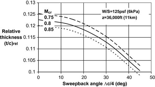
Figure 5.64 Relative thickness of a conventional airfoil as a function of quarter-chord sweepback for various Mach numbers at a wing loading of 125 lb/ft2 and an altitude of 36,000 ft.
5.7.4 Wing-mounted engines and a cranked trailing edge
If a cranked trailing edge at y = yb is desired, like that shown in Figure 5.3, then Equation (5.12) is used to determine the root chord. At this stage of the design, the market survey aircraft data should be used to help choose the location of the break in the trailing edge, yb. Typically the kink is placed just inboard of the engine location for wing-mounted engines. An estimate of the location of the engine may be developed from controllability considerations in emergency situations where one engine is shut down. We consider the specific case of a twin-engine aircraft; the approach may be readily extended to a four-engine airplane. The imbalance of thrust due to the shutdown of an engine on one side of the aircraft will induce a yawing moment N which must be countered by sufficient control authority from the rudder on the vertical tail. The restoring moment generated by the vertical tail is the product of the lift (side) force Lv produced by the vertical tail acting through the moment arm lv measured from the vertical tail aerodynamic center to the aircraft center of gravity as follows:
The yawing moment N may be estimated by noting that the available thrust Favail from the operating engine located at a spanwise station ye must be equal to the drag of the aircraft D at a new speed commanded by the pilot as follows:
Thus, for equilibrium flight, the yawing moment caused by thrust loss on one side of the aircraft must be balanced by a restoring moment provided by the vertical tail. Then, equating Equations (5.53) and (5.54) yields
Equation (5.55) introduces the volumetric coefficient of the vertical tail Vv which is discussed in more detail in the following chapter on tail design. We may rewrite this equation to show that an estimate for the spanwise location of an engine, in terms of the mean aerodynamic chord of the wing, is

The volume coefficient for the vertical tail of jet transports lies in the range 0.6 < Vv < 0.8, while the lift to drag ratio with one engine shut down will be about half the cruise value, that is, in the range 6 < (L/D) < 9. Because the lift coefficients of the tail and the airplane will be roughly proportional to their aspect ratios, a reasonable spanwise engine location is about 1.5cMAC. A more accurate result is developed in Chapter 6 and the engine location on the market survey aircraft may also be used to provide guidance at this stage in the design.
Engines mounted on the aft fuselage have much smaller yawing moments when an engine must be shut down because the effective moment arm for the thrust force is much smaller than for wing-mounted engines. This is an attractive safety feature of fuselage-mounted engines. In addition, because of their naturally greater ground clearance they better avoid foreign object damage due to ingestion by the engine inlet. However, the maintenance, repair, and overhaul expense for fuselage-mounted engines militates against their adoption, except for smaller jet transports, like regional jets, where there is insufficient ground clearance for wing-mounted turbofan engines. Interestingly, the Honda Jet has engines mounted above the wing to minimize ground clearance problems.
5.7.5 Placement of high lift devices
The location, type, chord size, and spanwise extent of the high lift devices is largely determined by meeting the lift coefficient requirements for takeoff and landing, as calculated in Chapter 4. Though the leading edge can support slats or flaps along most of the exposed span, there are constraints at engine pylon junctions for wing-mounted engines and at the wing root junctions. Trailing edge flaps have to share trailing edge space with low-speed (outboard) and possibly high-speed (inboard) ailerons as well as being clear of hot jet exhaust from wing-mounted engines. It is suggested that reasonable values of the trailing edge and leading edge flap layouts be chosen based on Figure 5.65 and on the market survey aircraft. For typical deflections the guidelines given in Table 5.7 should be considered.
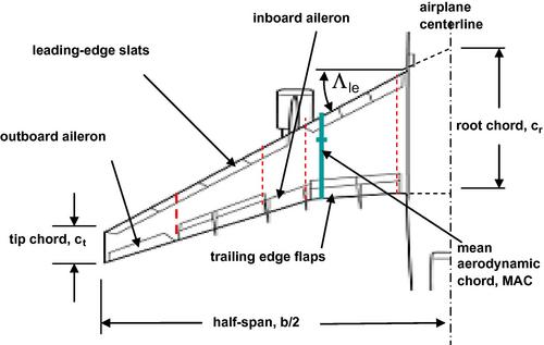
Typical Flap Settings for Different Configurations
| Flight Configuration | Flap Deflection δLE Leading Edge (deg) | Flap Deflection δTE Trailing Edge (deg) |
| Takeoff | 0–20 | 10–25 |
| Landing | 10–20 | 30–50 |
| Cruise | 0 | 0 |
5.7.6 Wingtip treatments
As described in the discussion of flow over finite wings in Appendix C, the trailing vortex sheet induces a swirling component into the flow field in the vicinity of the wing. At the same time it was demonstrated that the distribution of lift across the span influences the induced drag arising as a result of the trailing vortex sheet. The downwash at the lifting line tilts the velocity vector down by an amount equal to the induced angle of attack, tan-1(w/V). This in turn tilts the lift vector away from the normal to the free stream velocity producing a force component in the drag direction, and that component is the induced drag. Increasing the aspect ratio factor of the wing reduces the induced drag since the induced drag coefficient is
The aspect ratio is A = b2/S so the induced drag is proportional to the square of the span loading
![]()
Although this effect is beneficial it has drawbacks because increasing the span for the same lift effectively makes the wing more slender in planform leading to increased bending moment at the root of the wing. The increased bending moment must be countered by a strengthened structure which typically involves additional weight. By the same token, increased span can be a limiting factor in ground operations of commercial aircraft. Thus, the desire to improve the efficiency of aircraft by reducing wing drag has inherent limitations that must be considered.
The current rapid rise in fuel costs has made the search for drag reduction techniques even more important. Because induced drag is a large fraction of the total drag for subsonic aircraft, on the order of 35%, modifications of the spanwise lift distributions which reduce induced drag are desirable. Two wingtip treatments have received substantial attention from airplane manufacturers and operators: winglets and raked wingtips. These two types of wingtips are shown schematically in Figure 5.66. The winglet case presents a non-planar wing because the tips of the wing are not in the plane of the major portion of the wing. The raked wingtip presents a case of leading and trailing edges which are not straight although the wing remains planar.
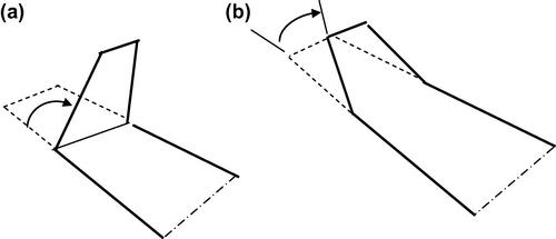
A number of different wingtip treatments aimed at improving aerodynamic performance are discussed in NRC (2007). The wide range of alterations to the outboard tenth of wings of operational aircraft illustrates the variety of design choices possible. However, the underlying concept is based on increasing the developed length of the wing, and this may be done in several ways:
• Increasing the span horizontally. Constraints include hangar, gate, taxiway, and runway width, increased structural weight of the wing, greater bending loads, and increased wetted area.
• Adding vertical, or canted, extensions at the wingtip above and/or below the plane of the wing. Constraints include increased wetted area and corner flow effects at junctions, increased weight and bending moments.
Kroo (2001) points out that various tip devices may lead to incremental but important gains in aircraft performance but there are challenges in integrating such features with the total aircraft system. In any case, the increased weight and cost of larger span wings leads to diminishing returns as span is increased. This, combined with the geometric issues noted above, determines the optimal span. Commercial experience with winglet retrofits on the Boeing 737, 757, and 767 aircraft indicates a fuel saving of up to around 5% for longer ranges.
5.7.7 Winglets
The flow around the tips of a finite wing involves a whirling motion caused by the difference in pressure between the upper and lower surfaces of the wing, as illustrated schematically in Figure 5.67. Therefore there is an inboard flow on the upper surface and an outboard flow on the lower surface. The swirling flow downstream of the trailing edge of the wing organizes, that is, “rolls up” itself into two concentrated trailing vortices after traveling a downstream distance on the order of the wingspan. It seems clear that preventing this motion would increase the total lift produced and a simple solution would appear to be the placement of endplates at each wingtip to block the cross-flow. However, this intuitive solution mainly increases drag because of the increased surface area needed, thereby eroding any benefit in improving lift. A more sophisticated exploitation of the three-dimensional flow field itself can indeed reduce the induced drag produced by the wing downwash.
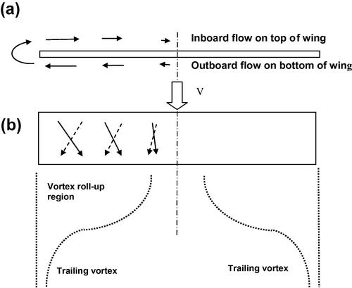
Figure 5.67 Schematic illustration of the flow over a finite lifting wing: (a) front view facing the leading edge showing cross-flow velocity components due to the higher pressures on the bottom wing surface and lower pressures on the top wing surface; (b) top view looking down on the wing illustrating the velocity on the top surface (solid arrows) and on the bottom surface (dashed arrows).
In much the same way that a sailboat may be sailed against the wind by appropriate pointing of the sail, the placement of a winglet in such a fashion as to actually produce a negative drag force, that is, a thrust, would be a distinct advantage. A view of the flow looking down on the upper surface of the wing with a winglet mounted vertically on the tip is shown in Figure 5.68. The resultant force in the flight direction produced by the three-dimensional flow on the winglet is given by
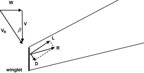
Figure 5.68 View looking down on the upper surface of the port wing showing the resultant velocity VR producing a resultant force R on the vertically mounted winglet, here represented as a simple flat plate. The magnitude of the angle β is exaggerated for clarity.
This force is a thrust force so that the drag of the wing is reduced. The actual design of the winglet is rather complicated and tends to have superior performance only in the vicinity of the design point chosen, for example, the cruise condition. Discussion of winglets may be found in textbooks on aerodynamics, for example McCormick (1995) and Bertin and Smith (1998). Early research on winglets applied to subsonic jet transports is reported by Flechner et al. (1976) and later studies are described by Lazos and Visser (2006). An interesting general discussion of the subject is presented by Jones (1979).
The important design variables for the winglet are
• the leading edge sweep angle of the winglet,
• the cant angle measured between the vertical and the plane of the winglet,
• the toe-in angle measured between the flight direction and the winglet root.
Installing a winglet doesn’t add the additional wing root bending moment that would be developed if the span was merely increased by the height of the winglet and this is a benefit. On the other hand, there are local forces and moments at the winglet junction with the wing and these tend to add some weight to the wing. Note that the action of the winglet is tied to properly exploiting the induced whirling flow generated by the finite wing so a winglet may be employed above the wing, below the wing, or both. The performance of a winglet is difficult to generalize in the preliminary design process and consideration of winglets is typically left to later detail design stages. In general, the induced drag reduction will not be equal to that provided by simply extending the wingspan by an amount equal to the winglet lengths, but perhaps by only half that amount. However, in recognition of their fairly widespread use they may be employed if desired, using market survey information as a guide. It is suggested that they be assumed to act aerodynamically as an increase in span equal to half the total length of the winglets. Furthermore, when the refined weight estimation procedures of Chapter 8 are carried out the weight of the wing with winglets should be considered to be equal to the weight of the wing with a span which includes the total length of the winglets.
5.7.8 Raked wingtips
Boeing has been prominent in the application of raked wingtips to their latest aircraft rather than winglets. The efforts at modifying the wingtips are aimed at altering the spanwise loading in order to achieve the desired reduction in induced drag. The idea may be broadly understood as taking a wing of given span and then increasing the span to achieve the corresponding reduction in the induced drag coefficient. This extended wingtip may be bent up to fashion a winglet or swept back further to form a raked wingtip. The details of the flow resulting from such changes are important to determining whether worthwhile improvements can be achieved. Of course, in addition to any performance improvements which may accrue to the wingtip treatment the other effects such as structural loading, weight implications, off-design performance, and the like must be assessed.
Rudolph (1991) patented a raked wingtip described as a modification to the main wing of a conventional airliner made by adding a highly tapered wingtip extension member to it. This addition increases the wingspan and aspect ratio with a relatively small increase in wetted area. Adding this extension and suitably changing the camber of the extension provides a means of tailoring the spanwise lift distribution into an almost elliptic shape so as to produce the least induced drag (as discussed in Appendix C) while incurring a minimal friction drag penalty.
A detailed computational and experimental study of raked wingtips is presented by Vijgen et al. (1989). They point out that the trailing vortex sheet behind a swept wing deforms rapidly and is not well described by classical wing theory as described in Appendix C. Nonlinear effects and non-planar attributes of the trailing vortex sheet must be treated by more sophisticated lifting surface methods. The performance improvements accruing to raked wingtips, or to winglets, are difficult to quantify in a general manner. Therefore, in the preliminary design stage, raked wingtips may be treated in the same empirical fashion as recommended for winglets. More accurate evaluation of their efficacy must be deferred to later stages of detailed design.
5.7.9 Wing dihedral and incidence
The configuration of the wing has been determined and now the disposition of the wing with respect to the fuselage is sought. The location of the wing along the longitudinal axis of the fuselage relative to the center of gravity of the complete aircraft is determined by stability and control requirements in pitch. However, the position of the center of gravity of the complete aircraft depends on where the wing is placed. Therefore setting the wing on the fuselage at this stage must be considered to be provisional. Locating the center of gravity position requires a fairly detailed knowledge of the weights and positions of all the major aircraft components. A refined weight estimate for the proposed aircraft along with the appropriate positioning of the wing is presented in Chapter 8.
Stability and control requirements in roll suggest that a certain amount of dihedral angle is desirable, as illustrated in Figure 5.69. This aspect of the airplane’s design is discussed in Chapter 6. An idea of the magnitude of the dihedral angle φ for typical airliners is presented in Table 5.5. Note that jet transports are low- or mid-wing aircraft and generally have dihedral angles of about 5–8°, while turboprop transports have no dihedral inboard of the engines and small values of dihedral, φ about 2°, on the section of the wing outboard of the engines, or even a small negative dihedral angle, generally called anhedral. Horizontal tail surfaces may also exhibit small values of dihedral or anhedral.
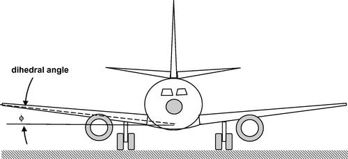
In order to ensure passenger comfort the cabin floor should remain essentially horizontal during cruising flight. Therefore the incidence angle i between a fuselage reference line, like the cabin floor, and the chord of the aircraft should be equal to the design angle of attack at the cruise condition, as illustrated in Figure 5.70. Typical values, as suggested by the database in Table 5.5, lie in the range of 2°<i<5°. During ground maneuvers the cabin floor is maintained level by the design of the landing gear. Obviously, during rotation and the subsequent climb the cabin floor will be tilted at the flight path angle. Such inclinations, like those due to banked turns, are generally small and acceptable to the passengers as routine. Because the lift required during cruise is not yet known in detail, the incidence angle, like the axial location of the wing, must remain a provisional value until the required lift is determined by the methods in Chapter 10.
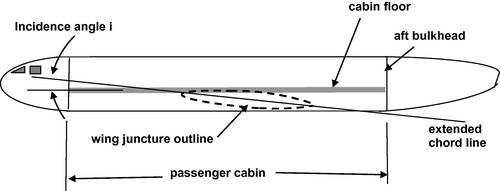
Figure 5.70 A typical elevation view of a fuselage illustrating the wing incidence angle i as measured between a fuselage reference line, taken here as the passenger cabin floor.
5.8 Design summary
The features of the wing designed for the proposed aircraft may now be collected for use in the further development of the design. The geometrical configuration of the wing of the proposed aircraft is now in hand, as well as the lifting characteristics in the takeoff, cruise, and landing configurations. These characteristics may be calculated by the methods described in this chapter in a relatively simple and rapid manner with little recourse to the computer outside of a spreadsheet. If desired, and if time and resources permit, the student may wish to explore CFD approaches for wing analysis. For example, the AVL code by Drela (2013) for the aerodynamic and flight-dynamic analysis of rigid aircraft of arbitrary configuration employs an extended vortex lattice model for the lifting surfaces, together with a slender-body model for fuselages and nacelles. It is available under the Gnu General Public License. The Computerized Environment for Aircraft Synthesis and Integrated Optimization Methods CEASIOM (2013) provides another available code that integrates computational tools for conceptual design.
The format illustrated in Table 5.8 is suggested for the presentation of the results for the maximum lift coefficients in the three basic configurations. Note that the numerical values shown in the sample table are merely representative of a typical design. It is expected that the maximum lift coefficients in takeoff and landing are appropriate to the requirements developed in selecting the engines in Chapter 4.
Summary of Estimated Values of CL,max
| Airfoil Choice: | NACA 64-212 (root) |
| NACA 64-209 (tip) | |
| Aspect Ratio: | A = 9.25 |
| Taper Ratio: | λ = 0.30 |
| Flap Type, cf/c: | Fowler, 23% |
| Spanwise Extent ηi and ηo: | 16.4% and 76.0% |
| Rated Area: | Swf/S = 0.53 |
| Configuration | δflap, Trailing Edge (deg) | δflap, Leading Edge (deg) | CL,max Low Speed M = 0.2 | CL,max Cruise Speed M = 0.8 |
| Cruise | 0 | 0 | 1.23 | 0.99 |
| Takeoff | 25 | 0 | 1.64 | – |
| Landing | 40 | 20 | 1.92 | – |
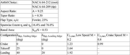
Note: Numbers in this table are merely representative.
The maximum lift coefficient for the cruise condition in Table 5.8, in combination with the lift curve slope of the wing determined by the methods in Section 5.3, the zero-lift angle of attack as given by the chosen airfoil section, and the angle of attack for maximum lift found using the methods of Section 5.4, provide a means for constructing a plot of CL as a function of α. These data will be used with the drag characteristics determined in Chapter 9 to compute the lift to drag ratio and the ceiling altitude of the aircraft in the cruise configuration. It is useful to calculate additional values of CLmax at different Mach numbers so as to develop a plot of CLmaxas a function of Mach number in the range 0.2 < M < Mcr so that the minimum flying speed of the aircraft at any altitude and Mach number may be calculated for the performance section of the report described in Chapter 10.
A scaled and dimensioned layout of the planform of the wing showing the location of engines, flaps, and other control devices is presented in Figure 5.50. These dimensions, along with the fuselage drawings and the tables prepared in this chapter, will be used in the design of the tail surfaces, which is discussed in the next chapter. The other features of the wing design should be presented in the manner illustrated by Table 5.9 which presents data for the wings of a representative range of commercial airliners for reference.
Wing Characteristics of Several Airliners. Other Features and Identification of Manufacturers are Given in Table 5.5
| Aircraft | Gross Weight (lb) Wg | Aspect Ratio A = b2/S | Sweep (deg) Λc/4 | Taper Ratio λ | MAC (ft) cmac | Root Thick. (t/c)r | Tip Thick. (t/c)t | Engine Loc. ye (ft) | Engine loc. ye/cmac |
| Q100 | 36,300 | 12.4 | 0.00 | 0.50 | 6.91 | 0.18 | 0.13 | 13.3 | 1.92 |
| Y-7 | 48,000 | 11.4 | 6.80a | 0.37 | 8.15 | 12.7 | 1.56 | ||
| ATR72-500 | 48,500 | 12.0 | 3.10a | 0.50 | 6.30 | 0.18 | 0.13 | 13.1 | 2.08 |
| ERJ145LR | 46,275 | 7.86 | 22.8 | 0.25 | 7.03 | 6.60 | 0.94 | ||
| CRJ200LR | 53,000 | 8.28 | 24.5 | 0.20 | 7.00 | 0.13 | 0.10 | 7.34 | 1.05 |
| CRJ700ER | 75,250 | 7.87 | 26.0 | 0.25 | 6.60 | 7.85 | 1.19 | ||
| E175 | 85,500 | 9.28 | 25.5 | 0.25 | 10.6 | 12.8 | 1.21 | ||
| B737-700ER | 154,500 | 10.3 | 25.0 | 0.22 | 13.5 | 16.0 | 1.17 | ||
| A320-200 | 169,800 | 9.35 | 25.0 | 0.23 | 13.3 | 0.15 | 0.11 | 18.3 | 1.37 |
| A310-300 | 361,600 | 8.79 | 28.0 | 0.20 | 19.1 | 0.21 | 0.11 | 25.3 | 1.32 |
| B767-200ER | 395,000 | 7.99 | 31.5 | 0.22 | 22.0 | 0.15 | 0.10 | 26.0 | 1.18 |
| B777-200 | 545,000 | 8.68 | 31.5 | 0.20 | 26.0 | 31.55 | 1.21 | ||
| A340-300 | 609,580 | 10.1 | 30.0 | 0.25 | 22.0 | 0.15 | 0.11 | 60.3b | 2.74 |
| B747-400 | 875,000 | 7.91 | 37.5 | 0.24 | 30.6 | 0.13 | 0.08 | 68.3bb | 2.23 |
| A380-800 | 1,234,600 | 7.53 | 35.8 | 0.20 | 40.3 | 0.15 | 0.12 | 84.3b | 2.09 |
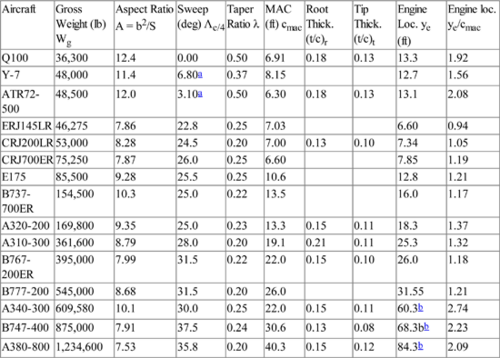
5.9 Nomenclature
A aspect ratio
a lift curve slope
b wingspan
c chord length
c’ chord length with slat extended
cd airfoil drag coefficient
cf flap chord
cl airfoil lift coefficient
clα airfoil lift curve slope
CL wing lift coefficient
CLα wing lift curve slope
Cp pressure coefficient
D drag
df wing diameter
e span efficiency factor
F thrust
g acceleration of gravity
i wing incidence angle
k constant
ka constant in Equation (5.50)
L lift
lw wing length
lv vertical tail moment arm
M Mach number
N yawing moment
Np number of passengers
p pressure
q dynamic pressure
R range
Re Reynolds number
Sv area of vertical tail
Sw,f wing planform area affected by flaps
Sw,s wing planform area affected by slats
sc/2 length of wing along the half-chord from root to tip
t thickness
V velocity
V* local sound speed
Vh horizontal tail volume coefficient
Vv vertical tail volume coefficient
v local velocity on airfoil
W weight
x chordwise distance from wing leading edge
y spanwise distance from centerline
yb spanwise distance to break in LE or TE sweepback
ye spanwise distance from centerline to engine centerline
α angle of attack
α0 angle of attack where a departs from linearity
β Prandtl-Meyer factor (1-M2)1/2 or sideslip angle
δ atmospheric pressure ratio or angular deflection
φ dihedral angle
γ ratio of specific heats
η y/(b/2)
ηmax empirical factor for leading edge radius, Equation (5.38)
ηδ empirical factor for slat deflection, Equation (5.38)
κ clα/2π
Λ wing sweepback angle
λ wing taper ratio
ρ density
σ atmospheric density ratio
σb wing root bending stress
θTC tail cone strike angle
5.9.1 Subscripts
base reference condition
cr cruise
crit critical
DD drag divergence
f flap
i induced or inboard
LE leading edge
l lower surface
MAC mean aerodynamic chord
max maximum
o outboard
p pressure
r root
ref reference condition
rel relative
s slat
SL sea level
TE trailing edge
t tip
to takeoff
u upper surface
0 zero-lift
References
1. Abbott, I.H. et al., 1945. Summary of Airfoil Data, NACA Technical Report No 824. Available from: <http://ntrs.nasa.gov/archive/nasa/casi.ntrs.nasa.gov/19930090976_1993090976.pdf>.![]()
2. Abbott IH, Von Doenhoff AE. Theory of Wing Sections. NY: Dover; 1959.
3. AGARD, 1979. Experimental Data Base for Computer Program Assessment: Report of the Fluid Dynamics Panel Working Group 04, AGARD-AR-138.
4. Allison, D.O., Mineck, R.E., 1996. Assessment of Dual-Point Drag Reduction for an Executive-Jet Modified Airfoil Section, NASA TP-3579.
5. Bertin JJ, Smith LM. Aerodynamics for Engineers. third ed. New Jersey: Prentice Hall; 1998.
6. Cahill, J.F., 1947. Two-Dimensional Wind-Tunnel Investigation of Four Types of High-Lift Flaps on an NACA 65–210 Airfoil Section, NACA TN 1191.
7. CEASIOM, 2013. Computerized Environment for Aircraft Synthesis and Integrated Optimization Methods. Available from: <www.ceasiom.com>![]() .
.
8. De Young, J., Harper, C.W., 1948. Theoretical Symmetric Span Loading at Subsonic Speeds for Wings Having Arbitrary Planforms, NACA Report 921.
9. Diederich, F.W., 1952. A Simple Approximate Method for Calculating Spanwise Lift Distributions and Aerodynamic Influence Coefficients at Subsonic Speeds. NACA TN 2751.
10. Drela M. XFOIL: an analysis and design system for low Reynolds number airfoils. In: Mueller TJ, ed. Lecture Notes in Engineering: Low Reynolds Number Aerodynamics. vol. 54. New York: Springer-Verlag; 1989 Available from: <http://web.mit.edu/drela/Public/web/xfoil/>![]() .
.
11. Drela, M., 2013. Available from: <http://web.mit.edu/drela/Public/web/avl/>.![]()
12. Dress, D.A., Stanewsky, E., McGuire, P. et al., 1984. High Reynolds Number Tests of the CAST 10–2/DOA 2 Airfoil in the Langley 0.3-Meter Transonic Cryogenic Tunnel – Phase II, NASA TM-86273.
13. Flechner, S.G., Jacobs, P.F., Whitcomb, R.T., 1976. A High Subsonic Speed Wind Tunnel Investigation of Winglets on a Representative Second Generation Jet Transport Wing, NASA Technical Note TN-8264.
14. Furlong, G.C., McHugh, J.G., 1953. A Summary and Analysis of the Low-Speed Longitudinal Characteristics of Swept Wings at High Reynolds Number, NACA Report 1339
15. Gottlieb, S.M., 1949. Two-Dimensional Wind-Tunnel Investigation of Two NACA 6-Series Airfoils with Leading-Edge Slats, NACA RM L8K22.
16. Green J, Quest J. A short history of the European transonic wind tunnel ETW. Progress in Aerospace Sciences. 2011;47(5):319-368.
17. Harper, C.W., Maki, R.L., 1964. A Review of the Stall Characteristics of Swept Wings, NASA TN D-2373.
18. Harris, C.D., 1990. NASA Supercritical Airfoils, NASA Technical Paper 2969. Available from: <http://hdl.handle.net/2002/13874>.![]()
19. Harris, C.D., 1975a. Aerodynamic Characteristics of the 10-Percent-Thick NASA Supercritical Airfoil 33 Designed for a Normal-Force Coefficient of 0.7, NASA TM X-72711.
20. Harris, C.D., 1975b. Aerodynamic Characteristics of a 14-Percent-Thick NASA Supercritical Airfoil Designed for a Normal-Force Coefficient of 0.7, NASA TM X-72712.
21. Harris, C.D., McGhee, R.J., Allison, D.O., 1980. Low Speed Aerodynamic Characteristics of a 14-Percent-Thick NASA Phase 2 Supercritical Airfoil Designed for a Lift Coefficient of 0.7, NASA TM -81912.
22. Hoak, D.E. et al., 1978. USAF Stability and Control DATCOM, Flight Control Division, Air Force Flight Dynamics Laboratory, Wright-Patterson AFB.
23. Hayter, N.L.F., Kelly, J.A., 1953. Lift and Pitching Moment at Low Speeds of the NACA 64A010 Airfoil Section Equipped with Various Combinations of a Leading Edge Slat, Leading Edge Flap, Split Flap and Double Slotted Flap, NACA TN 3007.
24. Jameson A. Computational Aerodynamics for Aircraft Design. Science. 1989;245:361-371.
25. Jenkins, R.V., 1983. Reynolds Number Tests of an NPL 9510 Airfoil in the Langley 0.3-Meter Transonic Tunnel, NASA TM-85663.
26. Jenkins, R.V., Johnson, Jr., W.G., Hill, A.S., et al., 1984. Data from Tests of a R4 Airfoil in the Langley 0.3-Meter Transonic Cryogenic Tunnel. NASA TM-85739.
27. Jenkinson, L.R., Simpkin, P., Rhodes, D., 1999. Civil Jet Aircraft Design, AIAA, Reston, VA.
28. Johnson Jr., W.G., Hill, A.S., 1985. Pressure Distributions From High Reynolds Number Tests of a Boeing BAC I Airfoil in the 0.3-Meter Transonic Cryogenic Tunnel, NASA TM-87600.
29. Johnson Jr., W.G., Hill, A.S., Eichmann, O., 1985. High Reynolds Number Tests of a NASA SC(3)-0712(B) Airfoil in the Langley 0.3-Meter Transonic Cryogenic Tunnel, NASA TM-86371.
30. Johnson, B.H., Shibata, H.H., 1951. Characteristics Throughout the Subsonic Speed Range of a Plane Wing and a Cambered and Twisted Wing, Both Having 45° of Sweepback, NACA RM A51D27.
31. Jones, R.T., 1947a. Wing Plan Forms for High-Speed Flight, NACA TR863.
32. Jones, R.T., 1947b. Effects of Sweepback on Boundary Layer and Separation, NACA TN 1402.
33. Jones RT. Minimizing Induced Drag. Soaring; 1979 pp. 26–29.
34. Koven, W., Graham, R.R., 1948. Wind Tunnel Investigation of High-Lift and Stall Control Devices Over A 37o Sweptback Wing of Aspect Ratio 6 at High Reynolds Numbers, NACA RM No L8D29.
35. Kroo I. Drag due to lift: concepts for prediction and reduction. Annual Reviews of Fluid Mechanics. 2001;33:587-617.
36. Ladson, C.L., 1996. Computer Program to Obtain Ordinates for NACA Airfoils, NASA Technical Memorandum 4741. Available from: <www.pdas.com>.![]()
37. Lazos, B.S., Visser, K.D., 2006. Aerodynamic Comparison of Hyper-Elliptic Cambered Span (HECS) Wings with Conventional Configurations, AIAA 2006–3469, 25th AIAA Applied Aerodynamics Conference, San Francisco.
38. Loftin, L.K., 1948. Theoretical and Experimental Data for a Number of NACA 6A-Series Airfoil Sections NACA, Report 903.
39. Loftin, L.K., Bursnall, W.J., 1948. The Effects of Variations in Reynolds Number between 3.0x10⁶ And 25.0x10⁶ upon the Aerodynamic Characteristics of a Number of 6-Series Airfoil Sections, NACA Technical Note No 1773.
40. Lovell, D.A., 1977. A Wind-Tunnel Investigation of the Effects of Flap Span and Deflection Angle, Wing Planform, and a Body on the High-Lift Performance of a 28o Swept Wing, RAE C.P. No 1372, Farnborough, UK.
41. McCormick BH. Aerodynamics, Aeronautics, and Flight Mechanics. NY: Wiley; 1995.
42. Mineck, R.E., Lawing, P.L., 1987. High Reynolds Number Tests of the NASA SC(2)-0012 Airfoil in the 0.3-Meter Transonic Cryogenic Tunnel, NASA TM-89102.
43. Morrison Jr., W.D., 1976. Advanced Airfoil Design: Empirically Based Transonic Aircraft Drag Buildup Technique NASA CR-137928.
44. NRC, 2007. Assessment of Wingtip Modifications to Increase the Fuel Efficiency of Air Force Aircraft, Air Force Studies Board, National Research Council, National Academy of Sciences, Washington, DC. Available from: <http://www.nap.edu/catalog/11839.html>.![]()
45. PDAS, 2013. Public Domain Aeronautical Software. Available from: <www.pdas.com/index.html>.![]()
46. Pearcy HH. The aerodynamic design of section shapes for swept wings. Advances in the Aeronautical Sciences. vol. 3. Oxford: Pergamon Press; 1962.
47. Phillips WF, Alley NR. Predicting maximum lift coefficient for twisted wings using lifting line theory. Journal of Aircraft. 2007;44(3):898-910.
48. Plentovich, E.B., Ladson, C.L., Hill, A.S., 1984. Tests of a NACA 651–213 Airfoil in the NASA Langley 0.3-Meter Transonic Cryogenic Tunnel, NASA TM-85732.
49. Rudolph, P.K.C., 1991. High Taper Wingtip Extension. US patent, No. 5,039,032.
50. Rudolph, P.K.C., 1996. High Lift Systems on Commercial Subsonic Airliners, NASA CR 4746.
51. Schiktanz, D., Scholz, D., 2011. Survey of Experimental Data of Selected Supercritical Airfoils, Airport2030-TN-Supercritical Airfoils. Available from: <http://www.fzt.haw-hamburg.de/pers/Scholz/Airport2030/Airport2030TN_Supercritical_Airfoils_11-12-21.pdf>.![]()
52. Scholz, D., Ciornei, S., 2005. Mach number, Relative Thickness, Sweep and Lift Coefficient of the Wing – An Empirical Investigation of Parameters and Equations, DGLR Paper No. 2005-122, in Jahrbuch 2005, Brandt, P. (Ed.), DGLR, Bonn, Germany.
53. Sharpes, D.E., 1985. Validation of USAF Stability and Control Datcom Methodologies for Straight-Tapered Swept-forward Wings, AFWAL-TR-84-3084, Flight Dynamics Laboratory Air Force Wright Aeronautical Laboratories.
54. Smith AMO. High lift aerodynamics, 37th Wright brothers lecture. Journal of Aircraft. 1975;12(6):501-530.
55. Whitcomb, R.T., Clark, L.R., 1965. An Airfoil Shape for Efficient Flight at Supercritical Mach Numbers, NASA TM X-1109.
56. Torenbeek E. Synthesis of Subsonic Airplane Design. Dordrecht, The Netherlands: Kluwer Academic Publishers; 1982.
57. UIUC, 2013. Airfoil Data Site. Available from: <http://www.ae.illinois.edu/m-selig/ads.html>.![]()
58. Valarezo WO, Chin VD. Method for the prediction of wing maximum lift. Journal of Aircraft. 1994;31(1):103-109.
59. Van Dam CP. The aerodynamic design of multi-element high-lift systems for transport airplanes. Progress in Aerospace Science. 2002;38(2):101-144.
60. Vijgen PMHW, Van Dam CP, Holmes B. Sheared wing-tip aerodynamics. Journal of Aircraft. 1989;26(3):207-213.
61. Wahls, R.A., 2001. The National Transonic Facility: A Research Retrospective, AIAA-2001-0754, 39th AIAA Aerospace Sciences Meeting and Exhibit.