
Spline Adaptive Filters
Theory and Applications
Michele Scarpiniti⁎; Danilo Comminiello⁎; Raffaele Parisi⁎; Aurelio Uncini⁎ ⁎Sapienza University of Rome, Rome, Italy
Abstract
In this chapter we propose a unifying overview of a recent class of nonlinear adaptive filters, known as Spline Adaptive Filter (SAF). This family of nonlinear adaptive filters comes from the general class of block-wise architectures consisting of a cascade of a suitable number of linear blocks and flexible memoryless nonlinear functions. In particular, the nonlinear function involved in the adaptation process is based on a spline function whose shape can be modified during the learning. Specifically, B-splines and Catmull–Rom splines are used, because they allow one to impose simple constraints on control parameters. The spline control points are adaptively changed using gradient-based techniques. In addition, in this chapter we show some of the most meaningful theoretical results in terms of upper bounds on the choice of the step sizes and excess mean square error values.
The SAF family of nonlinear adaptive filters can be successfully applied to several real-world applications, such as the identification of nonlinear systems, adaptive echo cancelers, adaptive noise control, nonlinear prediction and some other learning algorithms. Some experimental results are also presented to demonstrate the effectiveness of the proposed method.
Keywords
Nonlinear adaptive filters; Spline adaptive filters; Nonlinear cascade adaptive filters; Least mean square; Wiener systems; Hammerstein systems; Sandwich models
Chapter Points
- • We describe a nonlinear filtering approach based on spline nonlinear functions.
- • The proposed approach can be successfully used for the identification of nonlinear systems.
- • The proposed approach outperforms other approaches based on Volterra filters, both in speed of convergence and in performance.
- • We provide upper bounds on the choice of learning rates and the theoretical EMSE estimates.
Acknowledgements
This chapter has been partially supported by the PRIN2015 project no. 2015YPXH4W_004: “A green adaptive Fog computing and networking architecture (GAUChO)”, funded by the Italian MIUR, and by the project: “Vehicular Fog for energy-efficient QoS mining and dissemination of multimedia Big Data streams (V-FOG),” funded by Sapienza University of Rome.
3.1 Introduction
The theory of linear adaptive filtering (LAF) is well established in the literature [1–3]. In addition, the use of LAF methods for the solution of real-world problems is extensive and represents a central paradigm for many strategic applications [4]. The basic discrete-time linear adaptive filter model is made of a simple linear combiner whose length is determined by following some proper criterion and whose weights are adapted by choosing the most convenient optimization strategy [1].
In contrast, in many practical situations, the nature of the process of interest is often affected by any nonlinearity and thus requires the use of nonlinear adaptive filter (NAF) models. In the ideal case, if the nature of the nonlinearities is known a priori, it is possible to determine the NAF structure, in analogy with the mathematical model of nonlinearities. In this case the NAF is referred to as white-box (or structural) model and the process of adaptation consists of the estimation of the free model parameters (e.g., the coefficients of the nonlinear difference equation) [5].
On the contrary, if any a priori knowledge about the nature of nonlinearity is not available, it is preferred to use a black-box approach (functional model) [6,7]. In these cases, a unique framework for the solution does not exist and the existence of the solution cannot be guaranteed.
One of the best-known functional models that provide a good and general solution is based on the Volterra series [8]. Unfortunately, due to the large number of free parameters required, the Volterra adaptive filter (VAF) is generally employed only in situations of mild nonlinearity [8,9]. Neural networks (NNs) [10,11] represent another flexible tool to realize black-box NAFs, but they generally require a high computational cost and are not always feasible in online applications.
In the literature on nonlinear filtering, one of the most used structures is the so-called block-oriented representation, in which linear time-invariant (LTI) models are connected with memoryless nonlinear functions. The basic classes of block-oriented nonlinear systems are represented by the Wiener and Hammerstein models [12–14] and all those architectures originated by the connection of these two classes according to different topologies (i.e., parallel, cascade, feedback, etc. [15]). More specifically, the Wiener model consists of a cascade of an LTI filter followed by a static nonlinear function and sometimes it is known as linear–nonlinear (LN) model [16–19]. Conversely, the Hammerstein model consists of a cascade connection of a static nonlinear function followed by an LTI filter [20–22] and is sometimes indicated as nonlinear–linear (NL) model.
In a general nonlinear problem, with no a priori information available, the best adaptive model (Hammerstein or Wiener) is that most similar to the one to be identified. This fact implies that Wiener and Hammerstein models could be too restrictive in practical applications. Hence, other cascade models, such as the linear–nonlinear–linear (LNL) or the nonlinear–linear–nonlinear (NLN) models, were also introduced [12,23,24]. These cascade models, here called sandwich models, constitute a relatively simple but important class of nonlinear models that can approximate a wide class of nonlinear systems [25].
These models assume a key role in practical applications, since they are often related to specialized classes of nonlinear systems. As a matter of fact, these architectures can be successfully used in several applications in all fields of engineering [26], from circuit and system theory to modeling nonlinear characteristics of electronic devices and resistive networks [27–29], to signal processing [19,30], biomedical data analysis [31], digital communications [32,33] and even to hydraulics [34] and chemistry [35].
A crucial point in adopting a block-oriented model is the choice of the specific nonlinear function to be adopted. Obviously, several choices for this nonlinearity are possible, namely some invertible squashing functions, piece-wise linear functions [36,37,27], polynomial nonlinearities [38], splines [39] and more.
Recently a novel approach for the identification of Wiener, Hammerstein and sandwich models based on Spline Adaptive Filters (SAFs) has been proposed [30,40–44]. Among the advantages of these solutions, in order to yield great representative potential, high performance, low computational cost and easy implementability in dedicated hardware, all the nonlinearities involved in such systems are flexible and adapted by means of a fixed-length look-up table (LUT) that collects a suitable number of samples of the nonlinearity. Moreover, in order to have a continuous and derivable smooth function, the LUT samples are interpolated by a low-order uniform spline, like done in [40] for the Wiener SAF (WSAF), in [41] for the Hammerstein SAF (HSAF) and in [43] for the two sandwich SAFs (S1SAF and S2SAF).
SAFs have been successfully adopted in the literature in different scenarios, such as nonlinear echo cancellation [30] and active noise control [45–47], where signals are distorted by the low-cost hardware equipments. The standard LMS adaptation scheme has also been extended to the normalized version in [48] and to the maximum correntropy criterion [49]. The latter approach is particularly efficient in the case when data are corrupted by impulsive noise or contain large outliers. Finally, the SAF approach has been recently extended to the diffusion case [50], involving a network of distributed sensors.
In this chapter we aim at providing a deep and unifying overview of SAF models. After the description of the basic architectures and related learning algorithms, the main theoretical results on the choice of the step-size and the steady-state mean square error (MSE) are also provided. Finally some experimental results show the effectiveness of this family of nonlinear adaptive filters to solve real-world applications.
The rest of the chapter is organized as follows. Section 3.2 gives some background of spline interpolation. Section 3.3 provides a complete description of SAF models including the computational cost. Section 3.4 is devoted to the introduction of convergence results, while Section 3.5 provides some applicative scenarios and numerical results. Finally, Section 3.6 concludes the chapter.
3.1.1 Notation
In this chapter matrices are represented by boldface capital letters, i.e., ![]() , while
, while ![]() denotes the trace of a matrix. All vectors are column vectors, denoted by boldface lowercase letters, like
denotes the trace of a matrix. All vectors are column vectors, denoted by boldface lowercase letters, like ![]() , where
, where ![]() denotes the ith individual entry of w. In the recursive algorithm definition, a discrete-time subscript index n is added. For example, the weight vector, calculated according to some law, is written as
denotes the ith individual entry of w. In the recursive algorithm definition, a discrete-time subscript index n is added. For example, the weight vector, calculated according to some law, is written as ![]() . In the case of signal regression, vectors are indicated as
. In the case of signal regression, vectors are indicated as ![]() . Moreover, regarding the interpolated nonlinearity, the LUT control points are denoted
. Moreover, regarding the interpolated nonlinearity, the LUT control points are denoted ![]() , where
, where ![]() is the jth control point, while the ith span is denoted by
is the jth control point, while the ith span is denoted by ![]() . Finally, the Euclidean norm and the transpose of a vector are denoted by
. Finally, the Euclidean norm and the transpose of a vector are denoted by ![]() and
and ![]() , respectively.
, respectively.
3.2 Foundation of Spline Interpolation
Historically derived from elastic rulers that cross a certain number of points, called knots, and used in the past for technical drawing, splines are differentiable, up to a given order, polynomial curves for interpolation or approximation of a succession of ![]() knots inside a convex hull. The knots
knots inside a convex hull. The knots ![]() , for
, for ![]() , represent a tabulated function on the plane x-y [51,39,52] and, in order to construct an appropriate function, they are also constrained as
, represent a tabulated function on the plane x-y [51,39,52] and, in order to construct an appropriate function, they are also constrained as
Literature on splines is vast. Without loss of generality, in this brief review we consider the univariate basis or blending functions developed by Schoenberg, who introduced the name B-splines, deriving them from Bézier splines [51].
Let ![]() be the abscissa value between two consecutive knots. The spline curve is defined as an affine combination of some knots of a suitable P degree spline basis function
be the abscissa value between two consecutive knots. The spline curve is defined as an affine combination of some knots of a suitable P degree spline basis function ![]() with minimal support and certain continuity properties [52]:
with minimal support and certain continuity properties [52]:
Given ![]() knots, the univariate spline basis functions
knots, the univariate spline basis functions ![]() can be defined by the Cox–de Boor recursion [39]
can be defined by the Cox–de Boor recursion [39]
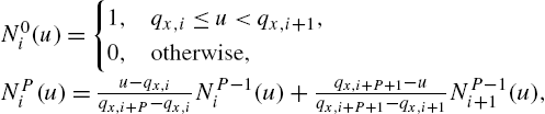
where ![]() . The blending functions
. The blending functions ![]() are polynomials of degree P with continuity of the first
are polynomials of degree P with continuity of the first ![]() derivatives. For example, for
derivatives. For example, for ![]() , we have
, we have
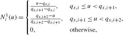
which results in a classical linear interpolation scheme, so ![]() is a rectangular function,
is a rectangular function, ![]() is a linear double-ramp function,
is a linear double-ramp function, ![]() is a quadratic double-ramp function. The generic
is a quadratic double-ramp function. The generic ![]() can be evaluated as a sequential convolution of P rectangular pulse functions
can be evaluated as a sequential convolution of P rectangular pulse functions ![]() .
.
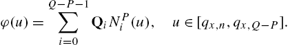
Hence, the curve (3.2) can be written as
where ![]() is a P degree local polynomial called curve span, entirely defined from
is a P degree local polynomial called curve span, entirely defined from ![]() knots, that are sometimes called control points. Moreover, scaling or translating the knot vector does not modify the basis functions, that can be fixed a priori for all control points.
knots, that are sometimes called control points. Moreover, scaling or translating the knot vector does not modify the basis functions, that can be fixed a priori for all control points.
From (3.4), there must be a unique mapping that allows us to calculate the local parameter u, as well as the proper curve span index i, from the global abscissa parameter (that in our case is the input sequence to the nonlinearity). In this way, we can represent any point lying on the curve ![]() as a point belonging to the single
as a point belonging to the single ![]() curve span.
curve span.
3.2.1 Uniform Cubic Spline
The recursive Eq. (3.3) can be entirely pre-calculated with considerable computational saving, by imposing a uniform distribution knot-vector, i.e., constant sampling step of the abscissa ![]() [39]. This implies that the local polynomial
[39]. This implies that the local polynomial ![]() in (3.4) can be written in a very simple form. A similar approach was successfully used in multilayer feed-forward neural networks [53].
in (3.4) can be written in a very simple form. A similar approach was successfully used in multilayer feed-forward neural networks [53].
Regarding the choice of the optimal degree P of a spline basis, a good compromise between flexibility and approximation behavior is represented by uniform cubic spline nonlinearities [54], as they provide good approximation capabilities avoiding the problem of over-fitting.
In the case of our interest where ![]() , the precalculation of the recursion (3.3) provides [39,54,53,40]
, the precalculation of the recursion (3.3) provides [39,54,53,40]
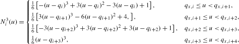
which can be reformulated in a matrix form as
for ![]() and
and ![]() and where the basis matrix C is defined as
and where the basis matrix C is defined as
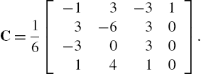
Imposing different constraints to the approximation relationship, several spline bases with different properties can be evaluated in a similar manner. An example of such a basis is the Catmull–Rom (CR) spline [55], very important in many applications. The interpolation scheme is the same of (3.5), while the CR-spline basis matrix C has the form
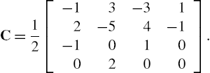
Note that CR-splines, initially developed for computer graphics purposes, represent a local interpolating scheme. The CR-spline, in fact, specifies a curve that passes through all of the control points, a feature which is not necessarily true for other spline methodologies. Overall, the CR-spline results in a more local approximation with respect to the B-spline.
For both the CR- and B-basis the curve has a continuous first derivative. For the B-spline the second derivative is also a continuous function, while for the CR spline the second derivative is not continuous at the knots. However, there is a regularization property common to most of the polynomial spline basis set (CR- and B-spline included) called variation diminishing property [39], which ensures the absence of unwanted oscillations of the curve between two consecutive control points, as well as the exact representation of linear segments.
Note also that the entries of the matrix C satisfy an important general property: the sum of all the entries is equal to one. This property is a direct consequence of the fact that the spline basis functions, derived from Bézier curves, are a generalization of the Bernstein polynomials and hence they represent a partition of unit (i.e., the sum of all basis function is one) [39,51].
In the next section, we present the main ideas on the SAFs and the derivation of the basic SAF models.
3.3 Spline Adaptive Filters
A Spline Adaptive Filter (SAF) consists of the cascade of a suitable number of linear filters and memoryless nonlinear functions obtained by the spline interpolation scheme described in Section 3.2.
In order to compute the nonlinear output ![]() , which is a spline interpolation of some adaptive control points contained in a LUT, we have to determine the explicit dependence between the input signal
, which is a spline interpolation of some adaptive control points contained in a LUT, we have to determine the explicit dependence between the input signal ![]() and
and ![]() . This can easily be done by considering that
. This can easily be done by considering that ![]() is a function of two local parameters
is a function of two local parameters ![]() and i that depend on
and i that depend on ![]() . From this onward we denote the local abscissa
. From this onward we denote the local abscissa ![]() with the subscript n in order to highlight the dependence on the input sample
with the subscript n in order to highlight the dependence on the input sample ![]() .
.
In the simple case of a uniformly spaced spline and a third-order (![]() ) local polynomial interpolator (adopted in this work), each spline segment, denoted span, is controlled by four (
) local polynomial interpolator (adopted in this work), each spline segment, denoted span, is controlled by four (![]() ) control points, also known as knots, addressed by the span index i that points at the first element of the related four points contained in the LUT. The computation procedure for the determination of the span index i and the local parameters
) control points, also known as knots, addressed by the span index i that points at the first element of the related four points contained in the LUT. The computation procedure for the determination of the span index i and the local parameters ![]() can be expressed by the following equations [53]:
can be expressed by the following equations [53]:
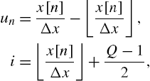
where ![]() is the uniform space between knots,
is the uniform space between knots, ![]() is the floor operator and Q is the fixed LUT length, i.e., the total number of control points. The second term on the right side of the second equation is an offset value needed to force i to be always nonnegative. Note that the index i depends on the time index n, i.e.,
is the floor operator and Q is the fixed LUT length, i.e., the total number of control points. The second term on the right side of the second equation is an offset value needed to force i to be always nonnegative. Note that the index i depends on the time index n, i.e., ![]() ; for simplicity of notation in the following we will write simply
; for simplicity of notation in the following we will write simply ![]() .
.
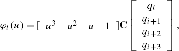
Referring to [40] and to [41] and with reference to (3.5), the output of the nonlinearity can be evaluated as
where the vector ![]() is defined as
is defined as ![]() ,
, ![]() is the precomputed matrix in (3.6) or (3.7), called spline basis matrix, and the vector
is the precomputed matrix in (3.6) or (3.7), called spline basis matrix, and the vector ![]() contains the control points at the instant n. More specifically,
contains the control points at the instant n. More specifically, ![]() is defined by
is defined by ![]() , where
, where ![]() is the kth entry in the LUT.
is the kth entry in the LUT.
It could be very important to compute the derivative of (3.9) with respect to its input. It is easily evaluated as
where ![]() .
.
The online learning algorithm can be derived by considering the cost function1 (CF) ![]() . In order to derive the LMS algorithm, this CF is usually approximated by considering only the instantaneous error
. In order to derive the LMS algorithm, this CF is usually approximated by considering only the instantaneous error
The expression of the error signal ![]() in (3.11) depends on the particular architecture used.
in (3.11) depends on the particular architecture used.
In the following subsections we provide the description of the four basic SAF architectures.
3.3.1 Wiener SAF
The Wiener SAF (WSAF) architecture consists of the cascade of a linear filter, represented by the filter coefficient weight vector ![]() , and a memoryless nonlinear function implemented by a spline interpolation scheme whose knots are denoted by the vector
, and a memoryless nonlinear function implemented by a spline interpolation scheme whose knots are denoted by the vector ![]() . The Wiener architecture is shown in Fig. 3.1, where
. The Wiener architecture is shown in Fig. 3.1, where ![]() denotes the output of the linear filter and it is the input to the spline function.
denotes the output of the linear filter and it is the input to the spline function.
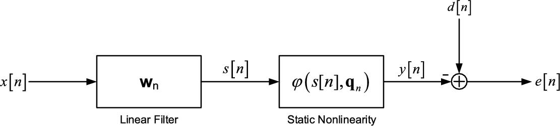
With reference to Fig. 3.1, let us define the output error ![]() as
as
where ![]() is the reference signal, i.e., the output of the model to be identified. The online learning algorithm can be derived by the minimization of (3.11). We proceed by applying the stochastic gradient adaptation [40], obtaining the LMS iterative algorithm
is the reference signal, i.e., the output of the model to be identified. The online learning algorithm can be derived by the minimization of (3.11). We proceed by applying the stochastic gradient adaptation [40], obtaining the LMS iterative algorithm
for the weights of the linear filter and
for the spline control points. The parameters ![]() and
and ![]() represent the learning rates for the weights and for the control points, respectively, and, for simplicity, incorporate the other constant values.
represent the learning rates for the weights and for the control points, respectively, and, for simplicity, incorporate the other constant values.
3.3.2 Hammerstein SAF
The Hammerstein SAF (HSAF) architecture consists of the cascade of a memoryless nonlinear function implemented by a spline interpolation scheme whose knots are denoted by the vector ![]() and a linear filter, represented by the filter coefficient weight vector
and a linear filter, represented by the filter coefficient weight vector ![]() . The Hammerstein architecture is shown in Fig. 3.2, where
. The Hammerstein architecture is shown in Fig. 3.2, where ![]() denotes the output of the nonlinear function.
denotes the output of the nonlinear function.
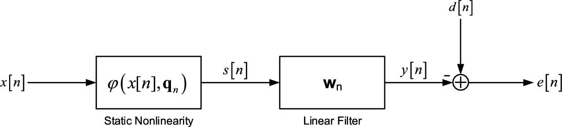
With reference to Fig. 3.2, we can define the output error ![]() as
as
where ![]() is the reference signal,
is the reference signal, ![]() , and each sample
, and each sample ![]() is evaluated by using (3.9).
is evaluated by using (3.9).
As in the Wiener case, the learning algorithm is derived by minimizing the CF (3.11). We proceed by applying the stochastic gradient adaptation as done in [41], obtaining the LMS iterative algorithm
for the weights of the linear filter and
for the spline control points. In (3.17), ![]() is a matrix which collects M past vectors
is a matrix which collects M past vectors ![]() , where each vector assumes the value of
, where each vector assumes the value of ![]() if evaluated in the same span i of the current sample input
if evaluated in the same span i of the current sample input ![]() or in an overlapped span; otherwise it is a zero vector.
or in an overlapped span; otherwise it is a zero vector.
As in the Wiener case, the learning rates ![]() and
and ![]() incorporate the other constant values.
incorporate the other constant values.
3.3.3 Sandwich 1 SAF
The Sandwich 1 (S1SAF) architecture [43] consists of the cascade of a memoryless nonlinear function implemented by a spline interpolation scheme whose knots are denoted by the vector ![]() , a linear filter, represented by the filter coefficient weight vector
, a linear filter, represented by the filter coefficient weight vector ![]() , and a second memoryless nonlinear function implemented by a spline interpolation scheme whose knots are denoted by the vector
, and a second memoryless nonlinear function implemented by a spline interpolation scheme whose knots are denoted by the vector ![]() . The S1 architecture is shown in Fig. 3.3, where
. The S1 architecture is shown in Fig. 3.3, where ![]() denotes the output of the first nonlinear function and
denotes the output of the first nonlinear function and ![]() is the output of the linear filter.
is the output of the linear filter.
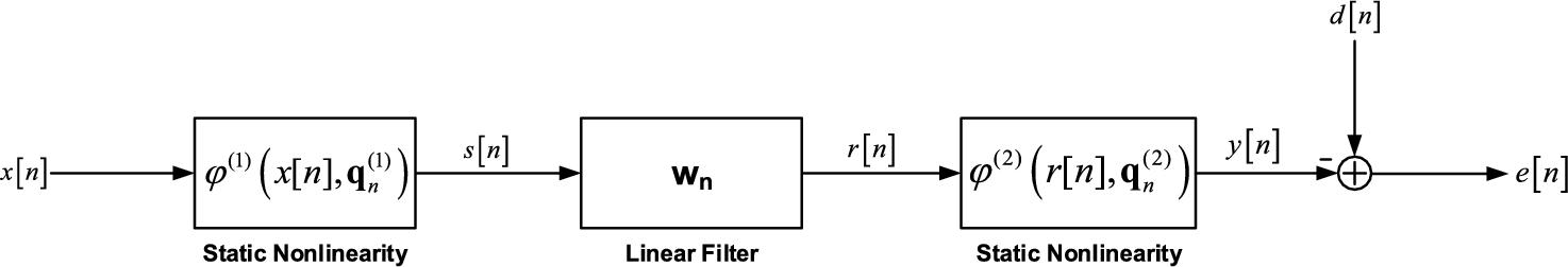
With reference to Fig. 3.3, we can define the output error ![]() as
as
where ![]() is the reference signal. As in the previous cases, the learning algorithm is derived by minimizing the CF (3.11). We proceed by applying the stochastic gradient adaptation as done in [43], obtaining the LMS iterative algorithm
is the reference signal. As in the previous cases, the learning algorithm is derived by minimizing the CF (3.11). We proceed by applying the stochastic gradient adaptation as done in [43], obtaining the LMS iterative algorithm
for the control points of the second nonlinearity,
for the weights of the linear filter and
for the control points of the first nonlinearity.
As in the previous cases, the learning rates ![]() ,
, ![]() and
and ![]() incorporate the other constant values.
incorporate the other constant values.
3.3.4 Sandwich 2 SAF
The Sandwich 2 (S2SAF) architecture [43] consists of the cascade of a linear filter, represented by the filter coefficient weight vector ![]() , a memoryless nonlinear function implemented by a spline interpolation scheme whose knots are denoted by the vector
, a memoryless nonlinear function implemented by a spline interpolation scheme whose knots are denoted by the vector ![]() and a second linear filter, represented by the filter coefficient weight vector
and a second linear filter, represented by the filter coefficient weight vector ![]() . The S2 architecture is shown in Fig. 3.4, where
. The S2 architecture is shown in Fig. 3.4, where ![]() denotes the output of the first linear filter and
denotes the output of the first linear filter and ![]() is the output of the nonlinear function.
is the output of the nonlinear function.
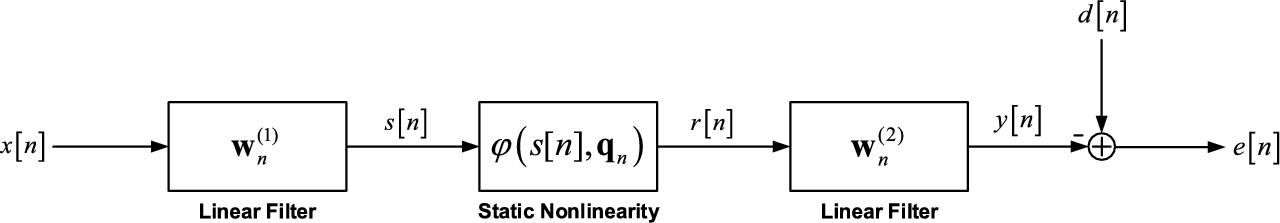
With reference to Fig. 3.4, we can define the output error ![]() as
as
where again ![]() is the reference signal. As in the previous cases, the learning algorithm is derived by minimizing the CF (3.11). We proceed by applying the stochastic gradient adaptation as done in [43], obtaining the LMS iterative algorithm
is the reference signal. As in the previous cases, the learning algorithm is derived by minimizing the CF (3.11). We proceed by applying the stochastic gradient adaptation as done in [43], obtaining the LMS iterative algorithm
for the weights of the second linear filter,
for the control points of the nonlinearity and
for the weights of the first linear filter.
As in the previous cases, the learning rates ![]() ,
, ![]() and
and ![]() incorporate the other constant values.
incorporate the other constant values.
3.3.5 Other Architectures
It is possible to derive other kinds of block-oriented architectures by suitable combinations of the basic architectures introduced in the previous subsections, thus obtaining particular cascade and/or parallel systems that can be successfully used to identify specific types of nonlinear systems or by using an IIR linear filter instead of a FIR one, like done in [42]. A more general situation of particular interest is the case of a convex (and affine) combination of the former architectures, like the ones proposed in [56] for another important class of nonlinear adaptive filters. In this scenario, the whole combined filter is able to automatically detect the subsystem that can provide better results. The extension of SAF to a combined scenario will be postponed to future works.
In a similar fashion, the work [46] introduces a hybrid nonlinear spline filter, which is designed as a cascade of an adaptive spline function and a single-layer adaptive nonlinear network, devoted to the problem of removing noise in the acoustic domain. Another work worthy to consider is [57], where the HSAF architecture is generalized to a Functional Link network. The proposed work shows very interesting results also in terms of classification ability.
Another type of generalization of SAFs is based on a suitable choice of the learning schemes. In most works, SAFs are adapted by using a general LMS strategy. However, this situation cannot be the best one. An extension to the more general normalized LMS (NLMS) is provided in [48], while the extension to the correntropy criterion can be found in [49]. The latter strategy is particularly useful when data are corrupted by impulsive noise or contain large outliers.
Finally, [50] derives a diffused version of the WSAF (D-SAF) by applying ideas from the Diffusion Adaptation (DA) framework. DA algorithms allow a network of agents to collectively estimate a parameter vector, by jointly minimizing the sum of their local cost functions. Experimental evaluations show that the D-SAF is able to robustly learn the underlying nonlinear model, with a significant gain compared with a noncooperative solution [50]. A detailed description of D-SAFs can be found in Chapter 9.
3.3.6 Computational Cost
From a computational point of view each SAF architecture requires the evaluation of two or three processing blocks. For each block the computational cost of the forward phase has to be evaluated (i.e., the evaluation of the system output) and also that of the backward phase (i.e., the adaptation of the adaptive system). It is well known from the literature that the computational cost of the LMS algorithm is ![]() multiplications plus 2M additions for each input sample [1], if M denotes the filter length.
multiplications plus 2M additions for each input sample [1], if M denotes the filter length.
In addition the cost of the spline evaluation must be considered. For each iteration only the ith span of the curve is modified by calculating the quantities ![]() , i and the expressions
, i and the expressions ![]() ,
, ![]() and
and ![]() . Note that the calculation of the quantity
. Note that the calculation of the quantity ![]() is executed during the output computation, as well as in the backward phase (the spline derivatives). However, most of the computations can be done through the reuse of past calculations (e.g., by explicating the polynomial and by use of the well-known Horner rule [58]). The cost for the spline output computation and its adaptation is
is executed during the output computation, as well as in the backward phase (the spline derivatives). However, most of the computations can be done through the reuse of past calculations (e.g., by explicating the polynomial and by use of the well-known Horner rule [58]). The cost for the spline output computation and its adaptation is ![]() multiplications plus
multiplications plus ![]() additions, where
additions, where ![]() and
and ![]() are constants (less than 16), depending on the implementation structure (see for example [53]). In any case, for high deep memory SAF, where the filter length is
are constants (less than 16), depending on the implementation structure (see for example [53]). In any case, for high deep memory SAF, where the filter length is ![]() , the computational overhead, for the nonlinear function computation and its adaptation, can be neglected with respect to a simple linear filter. It is straightforward to note that the computational cost can be further reduced by using some smart trick, like choosing the sampling step Δx or the learning rates
, the computational overhead, for the nonlinear function computation and its adaptation, can be neglected with respect to a simple linear filter. It is straightforward to note that the computational cost can be further reduced by using some smart trick, like choosing the sampling step Δx or the learning rates ![]() as a power of two. In fact, these constraints transform the multiplications into shift operations.
as a power of two. In fact, these constraints transform the multiplications into shift operations.
The total computational cost, inclusive of the forward and backward computation, for the presented four SAF architectures is summarized in Table 3.1. In this table M denotes the linear filter length. In the case of S2SAF architecture, ![]() and
and ![]() are the length of the first and second linear filter, respectively.
are the length of the first and second linear filter, respectively.
Table 3.1
| Additions | Multiplications | |
|---|---|---|
| WSAF | 2M + 48 | 2M + 67 |
| HSAF | 23M + 20 | 30M + 14 |
| S1SAF | 23M + 68 | 30M + 81 |
| S2SAF | 2M1M2 + M1 + 22M2 + 35 | 2M1M2 + 30M2 + 38 |
3.4 Convergence Properties
The convergence properties of the proposed learning algorithms could be evaluated in terms of their stability behavior, convergence speed, accuracy of the steady state and transient results and tracking ability as a function of their MSEs. For simplicity, in this chapter the attention is focused only on the optimal choice of the learning rates and the theoretical formulation of the excess MSE (EMSE) for the Wiener and Hammerstein architectures. Additional details and other useful results can be found in [40,41,43,44].
3.4.1 Bounds on the Learning Rates
A necessary but not sufficient condition for the algorithm convergence is the identification of a bound on the learning rate choice. These bounds on the learning rates can be derived by the Taylor series expansion of the error ![]() around the time index n, stopped at the first order. This series expansion involves the derivatives of the error with respect to the free parameters of the considered architecture.
around the time index n, stopped at the first order. This series expansion involves the derivatives of the error with respect to the free parameters of the considered architecture.
By performing these evaluations for the four SAF architectures introduced in Section 3.3 and by using the previous notation, we can easily obtain


The full derivation of these bounds can be found in [40,41,43].
3.4.2 Steady-State MSE
The aim of this paragraph is to evaluate the mean square performance of some of the proposed architectures at steady state. In particular, we are interested in the derivation of the EMSE of the nonlinear adaptive filter [2]. For simplicity we limit our analysis to the case of the Wiener and Hammerstein systems. The steady-state analysis is performed in a separate manner, by considering first the case of the linear filter alone and then the nonlinear spline function alone. Note that, since we are interested only in the steady state, the fixed subsystem in each substep can be considered adapted. The analysis is conducted by using a model of the same type of the used one, as shown in Fig. 3.5 for the particular case of the WSAF. Similar schemes are valid for the other kinds of architectures.
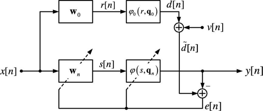
In the following we denote with ![]() the a priori error of the whole system, with
the a priori error of the whole system, with ![]() the a priori error when only the linear filter is adapted while the spline control points are fixed and similarly with
the a priori error when only the linear filter is adapted while the spline control points are fixed and similarly with ![]() the a priori error when only the control points are adapted while the linear filter is fixed. In order to make tractable the mathematical derivation, some assumption must be introduced:
the a priori error when only the control points are adapted while the linear filter is fixed. In order to make tractable the mathematical derivation, some assumption must be introduced:
A1. The noise sequence ![]() is independent and identically distributed with variance
is independent and identically distributed with variance ![]() and zero mean.
and zero mean.
A2. The noise sequence ![]() is independent of
is independent of ![]() ,
, ![]() ,
, ![]() ,
, ![]() and
and ![]() .
.
A3. The input sequence ![]() is zero mean with variance
is zero mean with variance ![]() and at steady state it is independent of
and at steady state it is independent of ![]() .
.
A4. At steady state, the error sequence ![]() and the a priori error sequence
and the a priori error sequence ![]() are independent of
are independent of ![]() ,
, ![]() ,
, ![]() ,
, ![]() ,
, ![]() and
and ![]() .
.
The EMSE ζ is defined at steady state as
Similar definitions hold for the EMSE ![]() due to the linear filter component
due to the linear filter component ![]() only and the EMSE
only and the EMSE ![]() due to the spline nonlinearity
due to the spline nonlinearity ![]() only.
only.
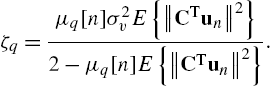
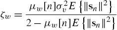
The MSE analysis has been performed by the energy conservation method [2]. Following the derivation presented in [41] and [44] we obtain an interesting property.
Proposition 1
The values of ![]() and
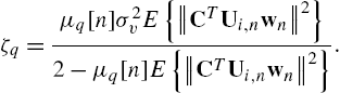
and ![]() are dependent on the particular SAF architecture considered. Specifically, for the Wiener case, we have [44]
are dependent on the particular SAF architecture considered. Specifically, for the Wiener case, we have [44]
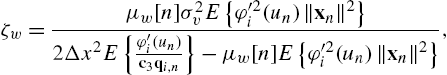
where ![]() is the third row of the C matrix and
is the third row of the C matrix and
Other useful properties on the steady-state performances of the WSAF can be found in [44]. For the Hammerstein case, we have [41]
and
3.5 Experimental Results
In order to validate the proposed nonlinear adaptive filtering solutions, several experiments were performed. In our previous works [40–44], several convergence tests showed the effectiveness of the proposed architectures in converging to the optimal solution. Moreover, these works also reported some experimental tests in system identification scenarios.2
In this section, we provide two kinds of experimental results on the identification of nonlinear systems: (i) tests taken from the literature on the field and (ii) tests on data measured from real-world applications.
3.5.1 Results From Simulated Scenarios
Regarding the experiments on nonlinear systems taken from the literature, we compare results obtained by SAFs with those of a full third-order Volterra adaptive filter [59] and the approach proposed by Jeraj and Mathews in [60] where the nonlinearity is implemented as a third-order polynomial. In addition, Sandwich architectures are also compared with the LNL approach proposed by Hegde et al. in [61,62]. In all experiments the input signal ![]() consists of 50 000 samples of the signal generated by the following relationship:
consists of 50 000 samples of the signal generated by the following relationship:
where ![]() is a zero mean white Gaussian noise with unitary variance and a (
is a zero mean white Gaussian noise with unitary variance and a (![]() ) is a parameter that determines the level of correlation between adjacent samples. Experiments were conducted with a set to 0.1 and 0.95. In addition an additive white noise
) is a parameter that determines the level of correlation between adjacent samples. Experiments were conducted with a set to 0.1 and 0.95. In addition an additive white noise ![]() with variance
with variance ![]() is considered.
is considered.
In the following we propose four tests in order to verify the Wiener, Hammerstein, Sandwich 1 and Sandwich 2 architectures described in Section 3.3. All the SAF models use a CR-spline basis in (3.7) with ![]() .
.
WSAF—The Wiener architecture to be identified is composed of the Back and Tsoi NARMA model reported in [63]. This model consists of a cascade of the third-order IIR filter
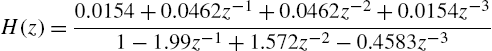
and the following nonlinearity:
The input signal ![]() is the colored signal obtained with (3.36), choosing
is the colored signal obtained with (3.36), choosing ![]() . The learning rates are set to
. The learning rates are set to ![]() and the filter length is
and the filter length is ![]() taps. The third-order Volterra filter has
taps. The third-order Volterra filter has ![]() filter taps and the learning rate is set to
filter taps and the learning rate is set to ![]() , while the Jeraj and Mathews architecture is characterized by
, while the Jeraj and Mathews architecture is characterized by ![]() ,
, ![]() , a nonlinearity of order
, a nonlinearity of order ![]() and learning rate
and learning rate ![]() . The MSE, averaged over 100 trials, is reported in Fig. 3.6A.
. The MSE, averaged over 100 trials, is reported in Fig. 3.6A.
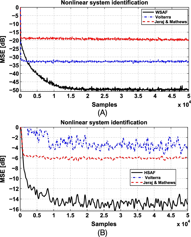
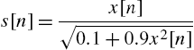
HSAF—The Hammerstein architecture to be identified, drawn from [64], is composed of the following nonlinearity:
where ![]() is the floor operator, and the FIR filter
is the floor operator, and the FIR filter ![]() . The learning rates are set to
. The learning rates are set to ![]() and
and ![]() , while the parameters of Volterra and Jeraj and Mathews architectures are the same as in the Wiener case. The MSE, averaged over 100 trials, is reported in Fig. 3.6B.
, while the parameters of Volterra and Jeraj and Mathews architectures are the same as in the Wiener case. The MSE, averaged over 100 trials, is reported in Fig. 3.6B.
S1SAF—The identification of a Sandwich 1 system is drawn from [65]. The first and last blocks are the following two static nonlinear functions:
and
while the second block is the following FIR filter:
The input signal ![]() is taken from (3.36) with
is taken from (3.36) with ![]() . Also
. Also ![]() dB is considered. The learning rates are set to
dB is considered. The learning rates are set to ![]() and the length is set to
and the length is set to ![]() . The proposed methods were compared with a standard full third-order Volterra filter, the approach of Jeraj and Mathews with the same parameters of the Wiener case and the LNL approach proposed by Hegde et al. with
. The proposed methods were compared with a standard full third-order Volterra filter, the approach of Jeraj and Mathews with the same parameters of the Wiener case and the LNL approach proposed by Hegde et al. with ![]() ,
, ![]() and
and ![]() . The MSE, averaged over 100 trials, is reported in Fig. 3.7A.
. The MSE, averaged over 100 trials, is reported in Fig. 3.7A.
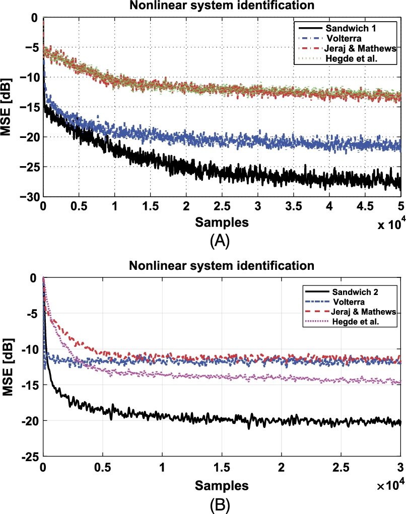
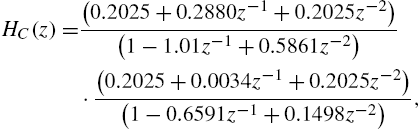
S2SAF—Finally, a Sandwich 2 to be identified is drawn from [66]. The first and last blocks are two fourth-order IIR filters, Butterworth and Chebyshev, respectively, with transfer functions
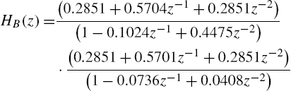
and
while the second block is the following nonlinearity:
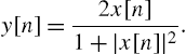
This system is similar to radio frequency amplifiers used in satellite communications (high-power amplifiers), in which the linear filters model the dispersive transmission paths, while the nonlinearity models the amplifier saturation. The input signal ![]() is as in (3.36) with
is as in (3.36) with ![]() . The learning rates are set to
. The learning rates are set to ![]() ,
, ![]() and
and ![]() and the lengths are set to
and the lengths are set to ![]() . Comparisons with Volterra, Jeraj and Mathews and Hegde et al. have been performed with the previous parameters. The MSE, averaged over 100 trials, is reported in Fig. 3.7B.
. Comparisons with Volterra, Jeraj and Mathews and Hegde et al. have been performed with the previous parameters. The MSE, averaged over 100 trials, is reported in Fig. 3.7B.
3.5.2 Results From Real-World Scenarios
In evaluating nonlinear architectures, it is important to test the performance of the proposed algorithm on completely unknown systems. For this purpose, we test our architecture from data sets collected from laboratory processes that can be described by block-oriented dynamic models. In particular, a number of interesting databases for system identification is represented by DaISy.3
From the DaISy database we have collected the following interesting and challenge data sets:
- • Exchanger [97-002]: the process is a liquid-saturated steam heat exchanger, where water is heated by pressurized saturated steam through a copper tube. The output variable is the outlet liquid temperature while the input variable is the liquid flow rate.
- • CD player arm [96-007]: data measured from the mechanical construction of a CD player arm. The input is the force of the mechanical actuators while the output is related to the tracking accuracy of the arm.
- • Thermic wall [96-011]: Heat flow density through a two-layer wall (brick and insulation layer). The input is the external temperature of the wall while the output is the heat flow density through the wall.
- • Heating system [99-001]: The experiment is a simple SISO heating system; the input drives a 300-Watt Halogen lamp, suspended several inches above a thin steel plate while the output is a thermocouple measurement taken from the back of the plate.
- • Continuous stirred tank reactor (CSTR) [98-002]: The process is a model of a CSTR, where the reaction is exothermic and the concentration is controlled by regulating the coolant flow. The input is the coolant flow while the output is the temperature.
All results have been compared with other state-of-the-art approaches used in previous experiments, namely a full third-order Volterra architecture [59] (with ![]() ), the LNL approach proposed by Hegde et al. in [61,62] (with
), the LNL approach proposed by Hegde et al. in [61,62] (with ![]() ), where the nonlinearity is implemented as a third-order polynomial and the approach proposed by Jeraj and Mathews in [60] (with
), where the nonlinearity is implemented as a third-order polynomial and the approach proposed by Jeraj and Mathews in [60] (with ![]() ,
, ![]() and
and ![]() ). In order to provide a fair comparison of the performance of such algorithms, Table 3.2 shows their asymptotic computational complexity.
). In order to provide a fair comparison of the performance of such algorithms, Table 3.2 shows their asymptotic computational complexity.
Table 3.2
| Algorithm | Asymptotic complexity |
|---|---|
| WSAF [40] |
|
| HSAF [41] |
|
| S1 SAF [43] |
|
| S2 SAF [43] |
|
| Third-order Volterra [59] |
|
| Hegde et al.[61] |
|
| Jeraj and Mathews [60] |
|
Moreover, we have chosen two additional measured data from coupled electric drives that consist of two electric motors that drive a pulley using a flexible belt and two measured data from a fluid level control system consisting of two cascaded tanks with free outlets fed by a pump. Additional details as regards these systems and data sets can be found in [67].
A last data set is taken from [68,69] and consist of the identification of a nonlinear electric circuit composed of the cascade of a third-order Chebyshev linear filter, a nonlinearity built by using a diode circuit and a second linear filter designed as a third-order inverse Chebyshev filter with a transmission of zero in the frequency band of interest.
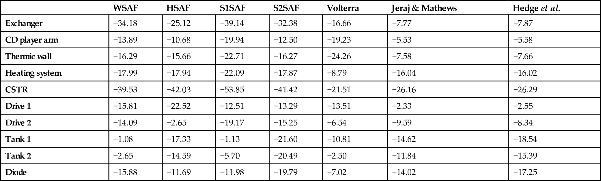
Results in terms of MSEs for all data sets are summarized in Table 3.3. It can be seen that the proposed SAF approaches provide the best performance in almost all cases.
Table 3.3
MSE in dB of the SAF architectures, compared with other referenced approaches, using real-world data
| WSAF | HSAF | S1SAF | S2SAF | Volterra | Jeraj & Mathews | Hedge et al. | |
|---|---|---|---|---|---|---|---|
| Exchanger | −34.18 | −25.12 | −39.14 | −32.38 | −16.66 | −7.77 | −7.87 |
| CD player arm | −13.89 | −10.68 | −19.94 | −12.50 | −19.23 | −5.53 | −5.58 |
| Thermic wall | −16.29 | −15.66 | −22.71 | −16.27 | −24.26 | −7.58 | −7.66 |
| Heating system | −17.99 | −17.94 | −22.09 | −17.87 | −8.79 | −16.04 | −16.02 |
| CSTR | −39.53 | −42.03 | −53.85 | −41.42 | −21.51 | −26.16 | −26.29 |
| Drive 1 | −15.81 | −22.52 | −12.51 | −13.29 | −13.51 | −2.33 | −2.55 |
| Drive 2 | −14.09 | −2.65 | −19.17 | −15.25 | −6.54 | −9.59 | −8.34 |
| Tank 1 | −1.08 | −17.33 | −1.13 | −21.60 | −10.81 | −14.62 | −18.54 |
| Tank 2 | −2.65 | −14.59 | −5.70 | −20.49 | −2.50 | −11.84 | −15.39 |
| Diode | −15.88 | −11.69 | −11.98 | −19.79 | −7.02 | −14.02 | −17.25 |
3.5.3 Applicative Scenarios
In the previous subsections, we provided some numerical results on the general problem of nonlinear system identification. However, SAFs have been used in applicative scenarios providing interesting and very good results.
A first applicative scenario is the nonlinear acoustic echo cancellation (NAEC) problem. The SAF approach has been successfully applied to NAEC in [30], where it is shown that the proposed solutions outperform other linear and nonlinear approaches.
Another challenging scenario is the nonlinear adaptive noise cancellation (NANC) problem. In particular, in [45] authors show the effectiveness of SAF approach to other state-of-the-art algorithms. Moreover, the proposed solution has been extended with additional refinements in [46] and [47].
Finally, as underlined in Section 3.3.5, the SAF approach has been recently extended to the diffusion case [50], involving a distributed (wireless) sensors network. The authors of this work derive a D-SAF by applying ideas from the DA framework, as explained in Chapter 9. Experimental evaluations on the D-SAF approach show that it is able to robustly learn the underlying nonlinear model, with a significant gain compared with a noncooperative solution.
3.6 Conclusion
In this chapter, a complete overview of a recent class of adaptive nonlinear filters, SAFs, has been provided. Specifically, we have described the basic block-oriented architecture implemented by SAFs, namely the Wiener, Hammerstein, NLN and LNL ones, as well as the related learning rules. Additionally, we have referred to the main theoretical results found in the literature on SAFs; the bounds on the choice of the learning rates and the theoretical evaluation of the EMSE for the Wiener and Hammerstein architectures.
Finally, after the introduction of some possible real-world applicative scenarios, some numerical results have shown the effectiveness of the proposed architectures.