
Maximum Correntropy Criterion–Based Kernel Adaptive Filters
Badong Chen⁎; Xin Wang⁎; Jose C. Principe⁎,† ⁎Institute of Artificial Intelligence and Robotics, Xi'an Jiaotong University, Xi'an, China
†University of Florida, Gainesville, FL, United States
Abstract
Kernel adaptive filters (KAFs) are a family of powerful online kernel learning methods that can learn nonlinear and nonstationary systems efficiently. Most of the existing KAFs are obtained by minimizing the well-known mean square error (MSE). The MSE criterion is computationally simple and very easy to implement but may suffer from a lack of robustness to non-Gaussian noises. To deal with the non-Gaussian noises robustly, the optimization criteria must go beyond the second-order framework. Recently, the correntropy, a novel similarity measure that involves all even-order moments, has been shown to be very robust to the presence of heavy-tailed non-Gaussian noises. A generalized correntropy has been proposed in a recent study. Combining the KAFs with the maximum correntropy criterion (MCC) provides a unified and efficient approach to handle nonlinearity, nonstationarity and non-Gaussianity. The major goal of this chapter is to briefly characterize such an approach. The KAFs under the generalized MCC will be investigated, and some simulation results will be presented.
Keywords
Kernel adaptive filters; Correntropy; Generalized correntropy; Maximum correntropy criterion; Robustness
Chapter Points
- • Kernel adaptive filters (KAFs) are powerful in online nonlinear system modeling.
- • Correntropy and generalized correntropy are local similarity measures, and the maximum correntropy criterion (MCC) is robust to impulsive non-Gaussian noises.
- • Combining KAFs and MCC provides an efficient way to deal with nonlinear modeling in the presence of non-Gaussian noises.
5.1 Introduction
The features of nonlinearity, nonstationarity and non-Gaussianity in many practical signals (such as EEG and EMG signals) pose great challenges for signal processing methods [1–5]. To deal with nonlinearities, a lot of nonlinear models were proposed in the literature. Well-known examples include neural networks (e.g., MLP, RBF), linear-in-the-parameter nonlinear models (e.g., Volterra series, kernel methods, extreme learning machines) and block-oriented nonlinear models (e.g., Wiener, Hammerstein) [6–10]. To handle nonstationarities, a common approach is to build the models in an online manner, where the parameters or structures of the models are updated adaptively to track the changes in a time varying process. For example, in adaptive filtering domains, various adaptive algorithms have been developed so far to learn the models adaptively, such as the least mean square (LMS), recursive least squares (RLS), affine projection algorithms (APA) and their variants [10–13]. To cope with non-Gaussianity, optimization criteria must go beyond the second-order framework, and statistical measures incorporating higher-order information should be used. In particular, information theoretic measures such as entropy, mutual information and divergences have been shown to be very efficient for extracting the non-Gaussian features of the processed data [14–17]. Recently, the concept of correntropy in information theoretic learning (ITL) has been successfully used for robust learning and signal processing in the presence of heavy-tailed non-Gaussian noises [18–27].
KAFs have recently attracted great attention due to their powerful learning capability for nonlinear and nonstationary system modeling [10,28–39]. The KAF algorithms are a family of online kernel learning methods, which are implemented as linear adaptive filters with input data being transformed into a high-dimensional feature space induced by a Mercer kernel [10]. Combining kernel methods with standard (linear) adaptive filtering algorithms, the KAFs have some desirable features such as universal approximation capability, the absence of local minima during adaptation and reasonable computational resources. To date, a number of kernel adaptive filtering algorithms have been developed, including kernel LMS (KLMS) [28], kernel RLS (KRLS) [29], kernel APA (KAPA) [36] and kernel Kalman filter [39]. Generally a KAF algorithm builds a growing RBF-like network with data-centered hidden nodes. In the literature, there are several approaches to constrain the network size of KAFs [10,31,40].
Most KAFs were developed under the popular mean square error (MSE) criterion, which is computationally simple and mathematically tractable but may suffer severe performance degradation in the presence of non-Gaussian noises. To improve the robustness of KAFs with respect to non-Gaussian noises, many efforts have been made to develop new KAF algorithms based on nonMSE (nonsecond-order) optimization criteria, such as the MCC [21,38], minimum error entropy (MEE) criterion [41], least mean p-power (LMP) criterion [42], least mean mixed norm (LMMN) criterion [43] and least mean kurtosis (LMK) criterion [44]. Increasing attention has recently been paid to the MCC criterion that aims at maximizing the correntropy between model output and desired response. Correntropy is a generalized correlation measure in kernel space and closely related to the Parzen estimator of Rényi's entropy [14], and its name comes from the words “correlation” and “entropy”. When used as an optimality criterion, correntropy has some desirable properties: smoothness, robustness and invexity [45,46]. Combining KAFs with MCC provides an efficient way to handle nonlinearity, nonstationarity and non-Gaussianity in a unified manner.
In this chapter, we give a brief introduction to the MCC-based KAFs. In Section 5.2, we briefly review two basic KAF algorithms. In Section 5.3, we introduce the concepts of correntropy and MCC. In Section 5.4, we present two KAF algorithms under the generalized MCC. Experimental results are shown in Section 5.5 and, finally, a conclusion is given in Section 5.6.
5.2 Kernel Adaptive Filters
Kernel methods are a powerful nonparametric modeling tool, which transform the input data into a high-dimensional feature space via a reproducing kernel such that the inner product operation in the feature space can be computed effectively through the kernel evaluation [47]. Using the linear structure of this feature space to implement a well-established linear adaptive filtering algorithm, one can obtain a KAF algorithm [10]. Among various KAF algorithms, the KLMS and KRLS are perhaps the most popular and widely used ones [28,29]. The KLMS is an LMS-type stochastic gradient–based learning algorithm which is computationally very simple yet efficient [28]. The KRLS is an RLS-type recursive learning algorithm which can outperform the KLMS in many practical situations but requires higher computational resources [10].
5.2.1 KLMS Algorithm
Consider the learning of a nonlinear function y=f(x)![]() based on the sample sequence {xi∈Rd,yi∈R}
based on the sample sequence {xi∈Rd,yi∈R}![]() , (i=1,2,...)
, (i=1,2,...)![]() . First, we transform the input data into a feature space F
. First, we transform the input data into a feature space F![]() through a nonlinear mapping φ(.)
through a nonlinear mapping φ(.)![]() induced by a Mercer kernel κ(.,.)
induced by a Mercer kernel κ(.,.)![]() . Then applying the well-known LMS algorithm [12] on the transformed sample sequence {φ(xi),yi}
. Then applying the well-known LMS algorithm [12] on the transformed sample sequence {φ(xi),yi}![]() , we have
, we have
Ωi=Ωi−1−μ∂∂Ωi−1e2i=Ωi−1+ηeiφ(xi),
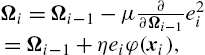
where Ωi![]() denotes the weight vector in feature space at iteration i, η=2μ
denotes the weight vector in feature space at iteration i, η=2μ![]() is the step size parameter and ei
is the step size parameter and ei![]() stands for the prediction error, that is,
stands for the prediction error, that is,
ei=yi−ΩTi−1φ(xi).
Identifying φ(x)=κ(.,x)![]() and Ωi=fi
and Ωi=fi![]() , where fi
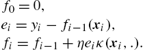
, where fi![]() denotes the estimated function at iteration i, and setting the initial function f0=0
denotes the estimated function at iteration i, and setting the initial function f0=0![]() , we can obtain the following update equations for KLMS [28]:
, we can obtain the following update equations for KLMS [28]:
f0=0,ei=yi−fi−1(xi),fi=fi−1+ηeiκ(xi,.).
Note that, for the reproducing kernel κ(.,.)![]() , we have 〈κ(.,x),fi〉F=fi(x)
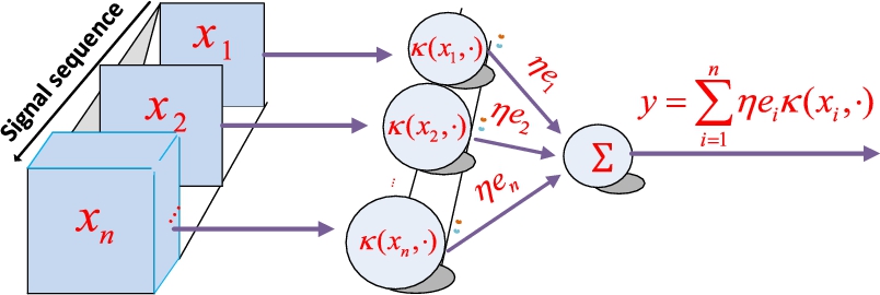
, we have 〈κ(.,x),fi〉F=fi(x)![]() . With a radial basis kernel (e.g., Gaussian kernel), the KLMS creates a growing RBF-like network [10], with the input vectors as the centers and prediction errors (scaled by η) as the output weights, as shown in Fig. 5.1.
. With a radial basis kernel (e.g., Gaussian kernel), the KLMS creates a growing RBF-like network [10], with the input vectors as the centers and prediction errors (scaled by η) as the output weights, as shown in Fig. 5.1.
5.2.2 KRLS Algorithm
Next, we present the KRLS algorithm [29]. Consider the following optimization cost function:
ℓ(Ω)=i∑j=1ζi−je2i+ζiγ‖Ω‖2,
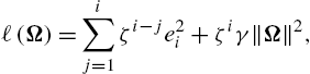
where ζ is the forgetting factor and γ is the regularization factor. Setting ∂∂Ωℓ(Ω)=0![]() , one can derive
, one can derive
Ω=(ΦiBiΦTi+γζiI)−1ΦiBiyi,
where Φi=[φ1,⋯,φi]![]() with φi
with φi![]() being φi=φ(xi)
being φi=φ(xi)![]() , yi=[y1,⋯,yi]
, yi=[y1,⋯,yi]![]() , I is an identity matrix and Bi=diag{ζi−1,ζi−2,⋯,1}
, I is an identity matrix and Bi=diag{ζi−1,ζi−2,⋯,1}![]() is a diagonal matrix. Using the matrix inversion lemma [10], we have
is a diagonal matrix. Using the matrix inversion lemma [10], we have
Ω=Φi(ΦTiΦi+γζiB−1i)−1yi.
Let ai=(ΦTiΦi+γζiB−1i)−1yi![]() be a coefficient vector. Then the weight vector Ω can be expressed explicitly as a linear combination of the transformed data, that is, Ω=i∑j=1(ai)jφj
be a coefficient vector. Then the weight vector Ω can be expressed explicitly as a linear combination of the transformed data, that is, Ω=i∑j=1(ai)jφj![]() , where (ai)j
, where (ai)j![]() denotes the jth component of ai
denotes the jth component of ai![]() . Denote Qi=(ΦTiΦi+γζiB−1i)−1
. Denote Qi=(ΦTiΦi+γζiB−1i)−1![]() . We have
. We have
Qi−1=[Qi−1−1hihiTφiTφi+γζi],
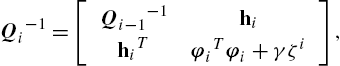
where hi=Φi−1Tφi![]() . Using the block matrix inversion identity [10], we have the following update rule for Qi
. Using the block matrix inversion identity [10], we have the following update rule for Qi![]() :
:
Qi=ri−1[Qi−1ri+ziziT−zi−ziT1],
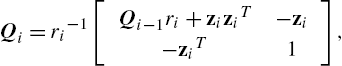
where zi=Qi−1hi![]() and ri=γζi+φiTφi−ziThi
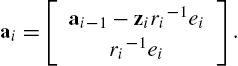
and ri=γζi+φiTφi−ziThi![]() . Therefore, the coefficient vector ai
. Therefore, the coefficient vector ai![]() can be updated as
can be updated as
ai=[ai−1−ziri−1eiri−1ei].
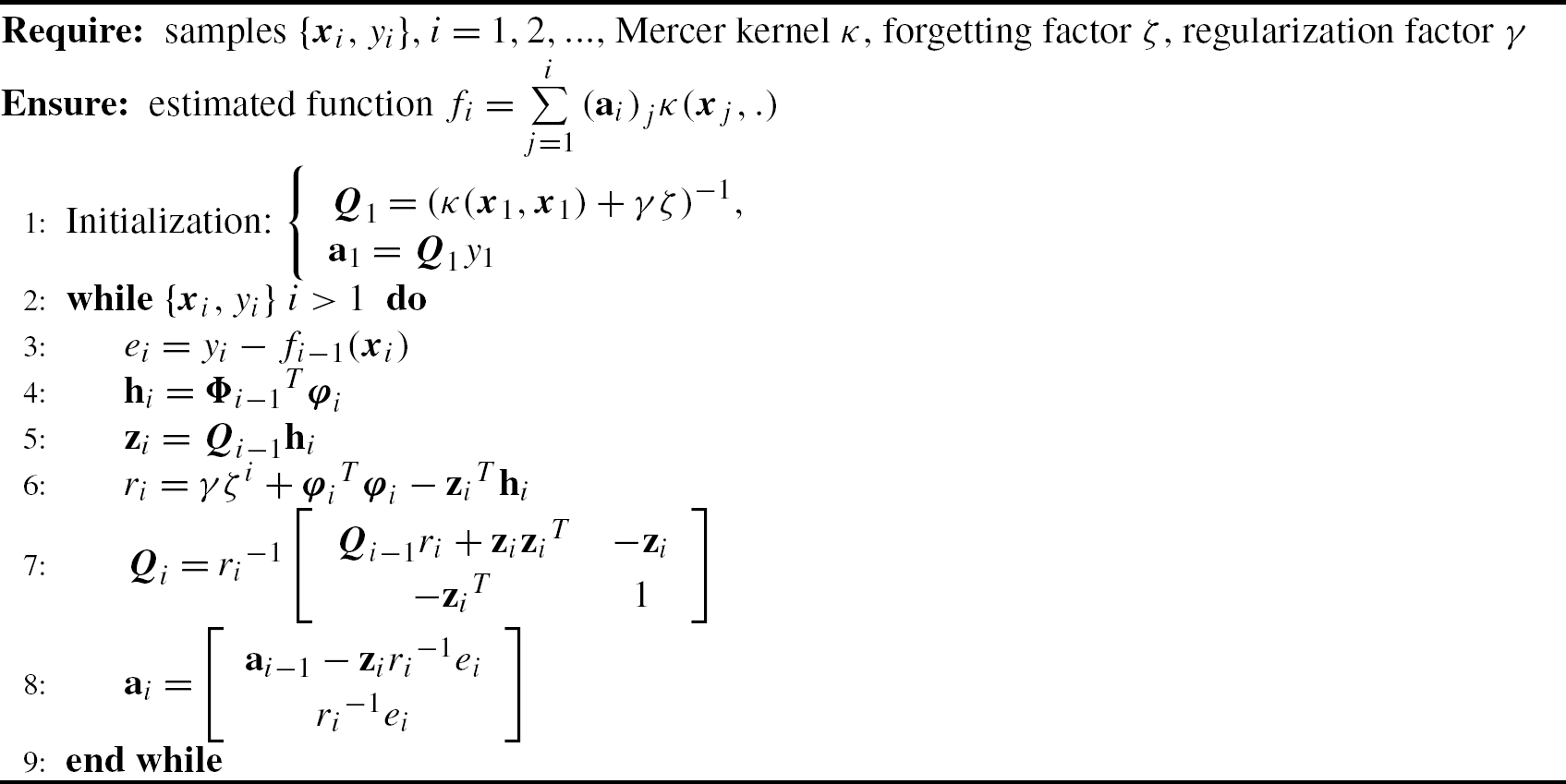
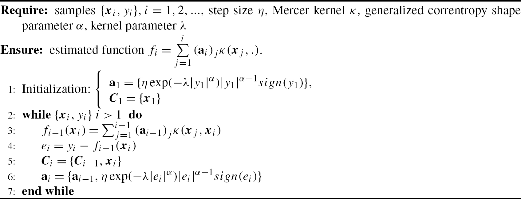
From the above derivation, the KRLS algorithm can be briefly described in Algorithm 1.
Similar to the KLMS, the KRLS also produces a growing RBF-like network. In order to reduce the computational cost and memory requirements of KAFs, several approaches have been proposed to curb the network growth [10]. Particularly, a simple online quantization approach was proposed in [31]. The basic idea of the quantization approach is to represent the input data with a smaller data set and quantize the original centers to the nearest code vector in the quantization code book (or dictionary).
5.3 Maximum Correntropy Criterion
5.3.1 Correntropy
First, we give some background on information theoretic learning (ITL) [14,15]. There is a close relationship between kernel methods and ITL. Most ITL cost functions, when estimated using the Parzen kernel estimator, can be expressed in terms of inner products in kernel space F![]() . For example, the Parzen estimator of the quadratic information potential (QIP) from samples x1,x2,⋯,xN∈R
. For example, the Parzen estimator of the quadratic information potential (QIP) from samples x1,x2,⋯,xN∈R![]() can be obtained as [14]
can be obtained as [14]
QIP(X)=1N2√2πσN∑i=1N∑j=1κσ(xi−xj),
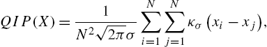
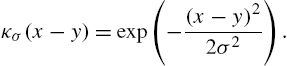
where κσ(.)![]() denotes the translation-invariant Gaussian kernel with bandwidth σ, given by
denotes the translation-invariant Gaussian kernel with bandwidth σ, given by
κσ(x−y)=exp(−(x−y)22σ2).
Since κσ(x,y)=〈φ(x),φ(y)〉F![]() , we have
, we have
QIP(X)=1√2πσ‖1NN∑i=1φ(xi)‖2F=1√2πσ〈1NN∑i=1φ(xi),1NN∑j=1φ(xj)〉F,
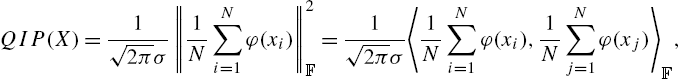
where ‖.‖F![]() stands for the norm in F
stands for the norm in F![]() . Thus, the estimated QIP represents the squared mean of the transformed data in kernel space.
. Thus, the estimated QIP represents the squared mean of the transformed data in kernel space.
The intrinsic link between ITL and kernel methods enlightens researchers to define new similarity measures in kernel space. As a local similarity measure in ITL, the correntropy between two random variables X and Y is defined [18] by
V(X,Y)=E[κσ(X−Y)]=∫κσ(x−y)dFXY(x,y),
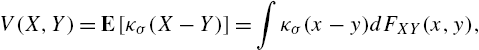
where the expectation value is over the joint distribution FXY(x,y)![]() . Correntropy can easily be estimated from data as
. Correntropy can easily be estimated from data as
V(X,Y)=1NN∑i=1κσ(xi−yi).
Correntropy can be expressed in terms of an inner product as
V(X,Y)=E[〈φ(X),φ(Y)〉F],
which is a generalized correlation measure in kernel space and itself is also positive definite, i.e., it defines a new kernel space for inference. In addition, by a simple Taylor series expansion on the kernel, one can see that correntropy provides a number that is the sum of all the statistical moments expressed by the kernel. In many applications this sum may be sufficient to quantify better than correlation the relationships of interest and it is much simpler to estimate than the higher-order statistical moments. Therefore, it can be considered as a new type of statistical descriptor. To date correntropy has been successfully applied to develop new adaptive filters for non-Gaussian noises [21–24], a correntropy MACE filter for pattern matching [48], robust PCA methods [19], new ICA algorithms [49], pitch detection [50] and nonlinear Granger causality analysis [51] methods with very good results. It is worth noting that many other similarity measures can be defined in kernel space such as the centered correntropy [14], correntropy coefficient [14], kernel risk sensitive loss [52] and kernel mean p-power error [53].
Based on the correntropy, one can define the correntropic loss (C-Loss) [52] as
CL(X,Y)=1−E[κσ(X−Y)],
which essentially is the MSE in kernel space since we have
CL(X,Y)=12E[‖φ(X)−φ(Y)‖2F].
The empirical C-Loss can be calculated by
ˆCL(X,Y)=1−1NN∑i=1κσ(xi−yi),
which is a function of the sample vectors X=[x1,x2,⋯,xN]T![]() and Y=[y1,y2,⋯,yN]T
and Y=[y1,y2,⋯,yN]T![]() . If no confusion can arise, we denote the empirical C-Loss by ˆCL(X,Y)
. If no confusion can arise, we denote the empirical C-Loss by ˆCL(X,Y)![]() . The square root of ˆCL(X,Y)
. The square root of ˆCL(X,Y)![]() is also called the Correntropy Induced Metric (CIM) between X
is also called the Correntropy Induced Metric (CIM) between X![]() and Y
and Y![]() since it defines a metric in the sample space [18].
since it defines a metric in the sample space [18].
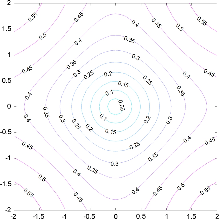
Fig. 5.2 shows the contours of distance from e=X−Y![]() to the origin in a two-dimensional space. The interesting observation from the figure is as follows. When two points are close, CIM behaves like an L2
to the origin in a two-dimensional space. The interesting observation from the figure is as follows. When two points are close, CIM behaves like an L2![]() norm (which is clear from the Taylor expansion of the kernel function) and we call this area the Euclidean zone; outside of the Euclidean zone CIM then behaves like an L1
norm (which is clear from the Taylor expansion of the kernel function) and we call this area the Euclidean zone; outside of the Euclidean zone CIM then behaves like an L1![]() , which is named the Transition zone; eventually in the Rectification zone as two points are further apart, the metric is much less sensitive to the change of the distance and saturates. Specifically, note that the CIM can be used in at least two respects for robust signal processing: (1) the relative insensitivity to very large values and the L1
, which is named the Transition zone; eventually in the Rectification zone as two points are further apart, the metric is much less sensitive to the change of the distance and saturates. Specifically, note that the CIM can be used in at least two respects for robust signal processing: (1) the relative insensitivity to very large values and the L1![]() equivalence in the transition region enables its use as an outlier-robust error measure and (2) its concave contours for large-norm vectors in the rectification regime can be used to further impose sparsity in adaptive system coefficients, which is typically done using an Lp(p≤1)
equivalence in the transition region enables its use as an outlier-robust error measure and (2) its concave contours for large-norm vectors in the rectification regime can be used to further impose sparsity in adaptive system coefficients, which is typically done using an Lp(p≤1)![]() norm penalization of the weight-vector norm. In both cases, the CIM has the useful property that for small-signal/weight situations the traditional quadratic measures are approximated, while for large-signal/weight conditions, it makes a smooth but sharp transition to desirable and robust Lp(p≤1)
norm penalization of the weight-vector norm. In both cases, the CIM has the useful property that for small-signal/weight situations the traditional quadratic measures are approximated, while for large-signal/weight conditions, it makes a smooth but sharp transition to desirable and robust Lp(p≤1)![]() penalization. The kernel size controls the speed of transition and can be optimally determined to best fit the data through the kernel density estimation connection. It is worth noting that there is a single parameter in correntropy, the kernel bandwidth, which controls the behavior of the CIM and MCC. Intuitively, if the data size is large and the problem dimension is low, a small kernel size can be used so that MCC searches with high precision (small bias) for the maximum position of the error PDF. However, if the data size is small and/or the problem dimension large, the kernel size has to be chosen so that the bulk of the data are inside the bandwidth to ensure efficient data usage while the outliers stay outside to enable an effective attenuation (small variance).
penalization. The kernel size controls the speed of transition and can be optimally determined to best fit the data through the kernel density estimation connection. It is worth noting that there is a single parameter in correntropy, the kernel bandwidth, which controls the behavior of the CIM and MCC. Intuitively, if the data size is large and the problem dimension is low, a small kernel size can be used so that MCC searches with high precision (small bias) for the maximum position of the error PDF. However, if the data size is small and/or the problem dimension large, the kernel size has to be chosen so that the bulk of the data are inside the bandwidth to ensure efficient data usage while the outliers stay outside to enable an effective attenuation (small variance).
The kernel function in correntropy can easily be extended to the generalized Gaussian function and the new measure is called the generalized correntropy [23]. Specifically, the generalized correntropy between random variables X and Y is defined by
Vα,β(X,Y)=E[Gα,β(X−Y)],
with Gα,β(.)![]() being the generalized Gaussian density (GGD) function [23]:
being the generalized Gaussian density (GGD) function [23]:
Gα,β(x)=α2βΓ(1/α)exp(−|xβ|α)=γα,βexp(−λ|x|α),
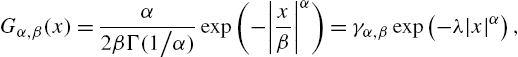
where Γ(.)![]() denotes the gamma function, α>0
denotes the gamma function, α>0![]() is the shape parameter, β>0
is the shape parameter, β>0![]() is the scale parameter, λ=1/βα
is the scale parameter, λ=1/βα![]() is the kernel parameter and γα,β=α/(2βΓ(1/α))
is the kernel parameter and γα,β=α/(2βΓ(1/α))![]() is the normalization constant. Obviously, when α=2
is the normalization constant. Obviously, when α=2![]() , the generalized correntropy is equivalent to the original correntropy. Note that the kernel function in the generalized correntropy is a Mercer kernel only when 0<α≤2
, the generalized correntropy is equivalent to the original correntropy. Note that the kernel function in the generalized correntropy is a Mercer kernel only when 0<α≤2![]() .
.
Similarly, one can define the generalized C-Loss (GC-Loss) and generalized CIM (GCIM). The GCIM also behaves like different norms (from Lα![]() to L0
to L0![]() ) of the data in different regions (see [23] for more details).
) of the data in different regions (see [23] for more details).
5.3.2 Maximum Correntropy Criterion
The correntropy and generalized correntropy can be used as an optimization cost in estimation-related problems. Given two random variables X∈R![]() , an unknown real-valued parameter to be estimated, and Y∈Rm
, an unknown real-valued parameter to be estimated, and Y∈Rm![]() , a vector of observations (measurements), an estimator of X can be defined as a function of Y:ˆX=g(Y)
, a vector of observations (measurements), an estimator of X can be defined as a function of Y:ˆX=g(Y)![]() , where g is solved by optimizing a certain cost function. Under the MCC, the estimator g can be solved by maximizing the correntropy (or minimizing the C-Loss) between X and ˆX
, where g is solved by optimizing a certain cost function. Under the MCC, the estimator g can be solved by maximizing the correntropy (or minimizing the C-Loss) between X and ˆX![]() , that is [45],
, that is [45],
gMCC=argmaxg∈GV(X,ˆX)=argmaxg∈GE[κσ(X−g(Y))],
where G stands for the collection of all measurable functions of Y. If ∀y∈Rm![]() , X has a conditional PDF pX|Y(x|y)
, X has a conditional PDF pX|Y(x|y)![]() , then the estimation error e=X−ˆX
, then the estimation error e=X−ˆX![]() has PDF
has PDF
pe(ε)=∫RmpX|Y(ε+g(y)|y)dFY(y),
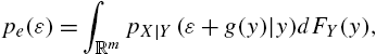
where FY(y)![]() is the distribution function of Y. It follows that
is the distribution function of Y. It follows that
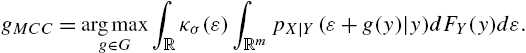
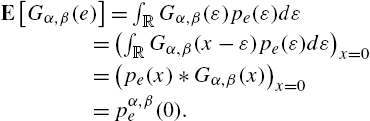
gMCC=argmaxg∈G∫Rκσ(ε)∫RmpX|Y(ε+g(y)|y)dFY(y)dε.
In [45], it has been proven that the MCC estimate is a smoothed maximum a posteriori probability (MAP) estimate, which equals the mode (at which the PDF attains its maximum value). Similar results hold for the generalized MCC (GMCC) estimation.
Theorem 1
Proof
It is easy to derive
Vα,β(X,ˆX)=∫RGα,β(ε)∫RmpX|Y(ε+g(y)|y)dFY(y)dε=∫Rm{∫∞−∞Gα,β(ε)pX|Y(ε+g(y)|y)dε}dFY(y)=∫Rm{∫∞−∞Gα,β(ε′−g(y))pX|Y(ε′|y)dε′}dFY(y)(a)=∫Rm{∫∞−∞Gα,β(g(y)−ε′)pX|Y(ε′|y)dε′}dFY(y)=∫Rm{(Gα,β(.)⁎pX|Y(.|y))(g(y))}dFY(y)=∫Rmρα,β(g(y)|y)dFY(y),
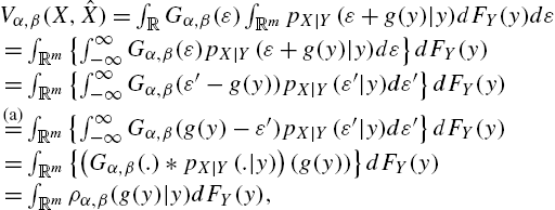
where ε′=ε+g(y)![]() and (a) comes from the symmetry of Gα,β(.)
and (a) comes from the symmetry of Gα,β(.)![]() . Thus
. Thus
gGMCC=argmaxg∈G∫Rmρα,β(g(y)|y)dFY(y)⇒gGMCC(y)=argmaxx∈Rρα,β(x|y),∀y∈Rm
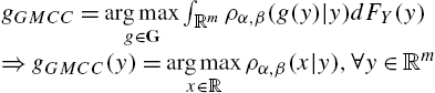
This completes the proof.
Remark
Considering the conditional PDF pX|Y(x|y)![]() as an a posteriori PDF given the observation y, the function ρα,β(x|y)
as an a posteriori PDF given the observation y, the function ρα,β(x|y)![]() is a smoothed (by convolution) a posteriori PDF. Therefore, the GMCC estimate is a smoothed MAP estimate.
is a smoothed (by convolution) a posteriori PDF. Therefore, the GMCC estimate is a smoothed MAP estimate.
Corollary 1
When β→0+![]() (or λ→∞
(or λ→∞![]() ), the GMCC estimation becomes the MAP estimation.
), the GMCC estimation becomes the MAP estimation.
Proof
As β→0+![]() , the GGD function Gα,β(.)
, the GGD function Gα,β(.)![]() will approach the Dirac delta function and the smoothed conditional PDF ρα,β(x|y)
will approach the Dirac delta function and the smoothed conditional PDF ρα,β(x|y)![]() will reduce to the original conditional PDF pX|Y(x|y)
will reduce to the original conditional PDF pX|Y(x|y)![]() . In this case, the GMCC estimation will be equivalent to the MAP estimation.
. In this case, the GMCC estimation will be equivalent to the MAP estimation.
Theorem 2
Proof
Theorem 3
When β→∞![]() (or λ→0+
(or λ→0+![]() ), the GMCC estimation will be equivalent to the LMP estimation with p=α
), the GMCC estimation will be equivalent to the LMP estimation with p=α![]() .
.
Proof
Under the LMP criterion, the optimal estimator is solved by minimizing the mean p-power of the error:
gLMP=argming∈GE[|e|p].
On the other hand, we have Vα,β(X,ˆX)≈γα,β(1−λE[|e|α])![]() as λ→0+
as λ→0+![]() . It follows that
. It follows that
maxVα,β(X,ˆX)∼minE[|e|α],
that is, as λ→0+![]() , the GMCC estimation will be, approximately, equivalent to the LMP estimation with p=α
, the GMCC estimation will be, approximately, equivalent to the LMP estimation with p=α![]() .
.
5.4 Kernel Adaptive Filters Under Generalized MCC
Most of the KAFs, such as KLMS and KRLS, have been derived under the well-known MSE criterion. The MSE is computationally simple and mathematically tractable but may perform very poorly under non-Gaussian noise (especially impulsive noise) disturbance. An efficient approach to improve the robustness to non-Gaussian noises is to use the MCC-based costs [21–24]. In the following, we present two KAF algorithms under the generalized MCC [54,55]. Of course, one can derive many other KAFs under GMCC.
5.4.1 Generalized Kernel Maximum Correntropy
In a way very similar to the derivation of KLMS, applying the GMCC on the transformed sample sequence {φ(xi),yi}![]() , one can derive
, one can derive
Ωi=Ωi−1+μ∂∂Ωi−1exp(−λ|ei|α)=Ωi−1+μλαexp(−λ|ei|α)|ei|α−1sign(ei)φ(xi)=Ωi−1+ηexp(−λ|ei|α)|ei|α−1sign(ei)φ(xi),
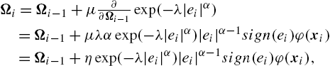
where the step size η=μλα![]() . The above algorithm is called the generalized kernel maximum correntropy (GKMC) [54]. From (5.32), we have the following observations:
. The above algorithm is called the generalized kernel maximum correntropy (GKMC) [54]. From (5.32), we have the following observations:
1) When α=2![]() , the GKMC becomes
, the GKMC becomes
Ωi=Ωi−1+ηexp(−λe2i)eiφ(xi),
which is the kernel maximum correntropy (KMC) algorithm developed in [21].
2) When λ→0+![]() , the GKMC becomes
, the GKMC becomes
Ωi=Ωi−1+η|ei|α−1sign(ei)φ(xi),
which is the kernel LMP (KLMP) algorithm developed in [42].
3) When α=2![]() and λ→0+
and λ→0+![]() , the GKMC will reduce to the KLMS algorithm
, the GKMC will reduce to the KLMS algorithm
Ωi=Ωi−1+ηeiφ(xi).
In addition, one can rewrite (5.32) as
Ωi=Ωi−1+ηieiφ(xi),
where ηi=ηexp(−λ|ei|α)|ei|α−2![]() is a variable step size (VSS). Thus, the GKMC can be viewed as a KLMS with VSS ηi
is a variable step size (VSS). Thus, the GKMC can be viewed as a KLMS with VSS ηi![]() . Since ηi→0
. Since ηi→0![]() as |ei|→∞
as |ei|→∞![]() , the learning rate of GKMC will approach zero when a large error occurs. This property ensures the robustness of the GKMC with respect to large outliers.
, the learning rate of GKMC will approach zero when a large error occurs. This property ensures the robustness of the GKMC with respect to large outliers.
In summary, the GKMC algorithm is summarized in Algorithm 2, where ai![]() denotes the coefficient vector at iteration i, (ai)j
denotes the coefficient vector at iteration i, (ai)j![]() is the jth component of ai
is the jth component of ai![]() and Ci
and Ci![]() is the center set (or dictionary).
is the center set (or dictionary).
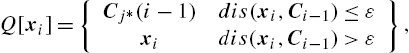
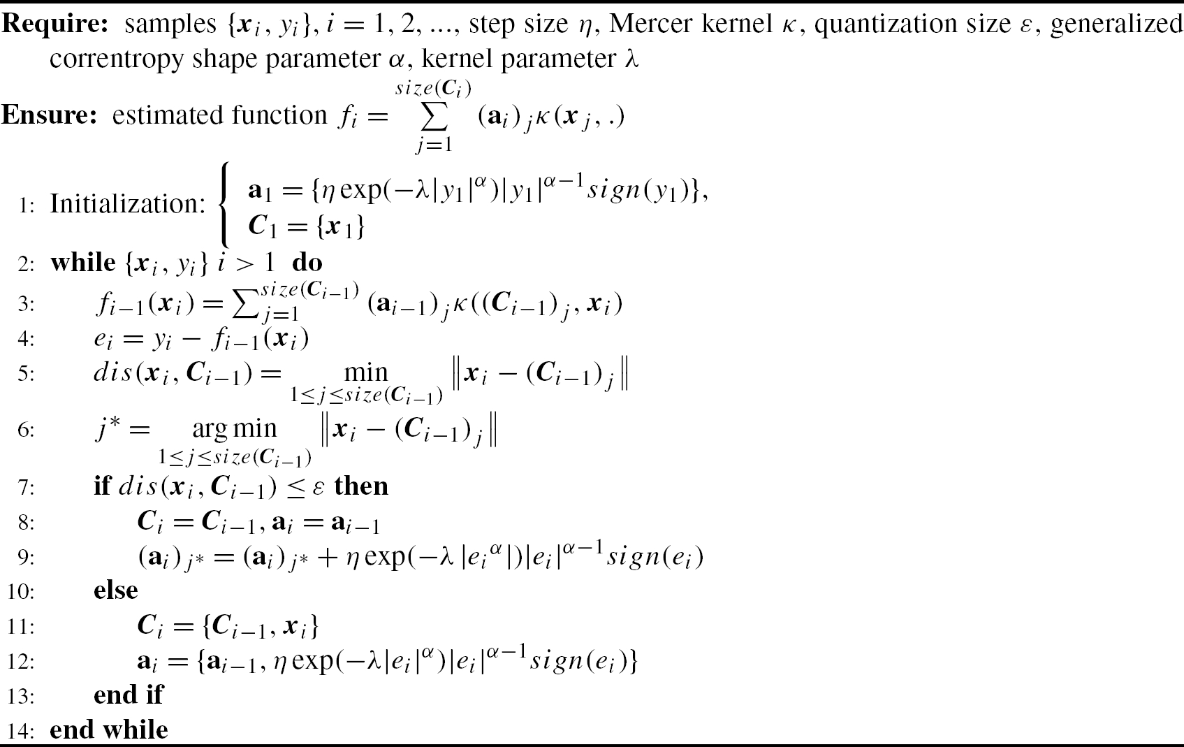
The network size of the GKMC grows linearly with the number of input data. One can use a simple quantization approach to curb the network growth [31]. In this way, the weight update Eq. (5.32) becomes
Ωi=Ωi−1+ηexp(−λ|ei|α)|ei|α−1sign(ei)φ(Q[xi]),
where Q[.]![]() denotes the quantization operator [31]:
denotes the quantization operator [31]:
Q[xi]={Cj⁎(i−1)dis(xi,Ci−1)≤εxidis(xi,Ci−1)>ε},
with Ci−1![]() being the codebook at iteration i−1
being the codebook at iteration i−1![]() , ε the quantization size and dis(xi,Ci−1)
, ε the quantization size and dis(xi,Ci−1)![]() the distance between xi
the distance between xi![]() and Ci−1
and Ci−1![]() . We have
. We have
dis(xi,Ci−1)=min1≤j≤size(Ci−1)‖xi−(Ci−1)j‖,
where (Ci−1)j![]() denotes the jth element (code vector) of the codebook Ci−1
denotes the jth element (code vector) of the codebook Ci−1![]() , j⁎
, j⁎![]() is the index of the closest center
is the index of the closest center
j⁎=argmin1≤j≤size(C(i−1))‖xi−(Ci−1)j‖.
The quantized GKMC (QGKMC) algorithm is summarized in Algorithm 3.
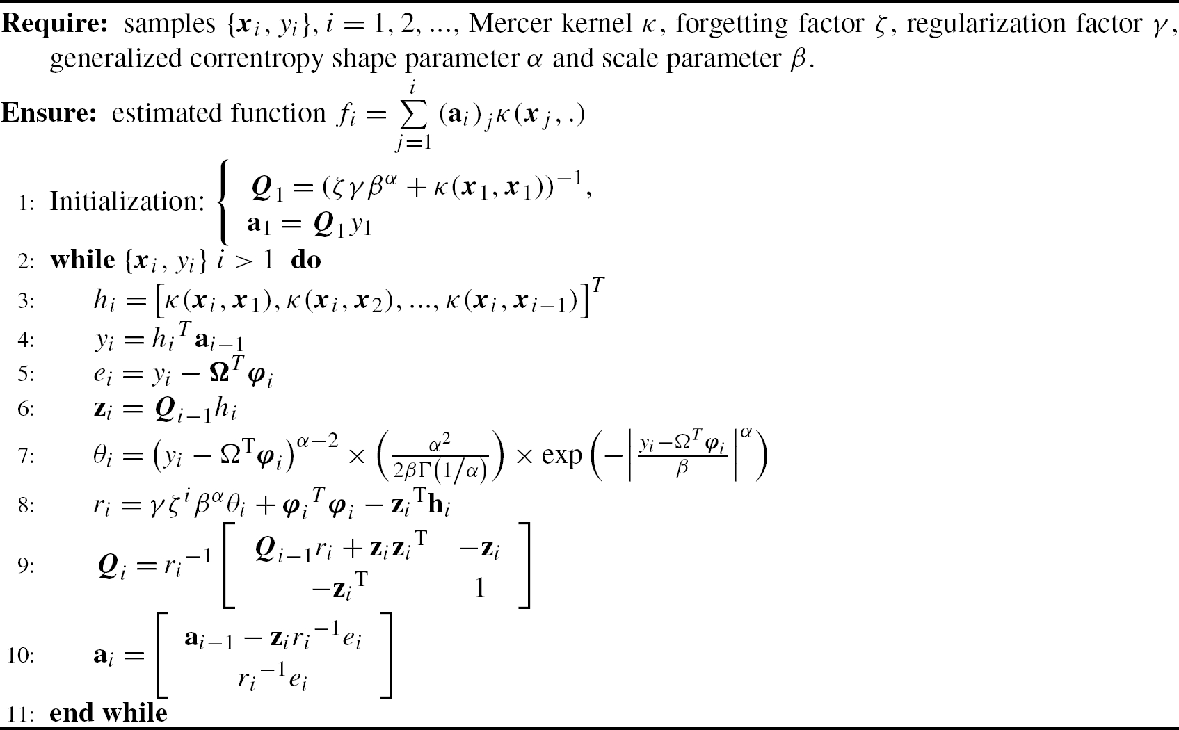
5.4.2 Generalized Kernel Recursive Maximum Correntropy
Next, we derive the generalized kernel recursive maximum correntropy (GKRMC) algorithm [55]. A weighted and regularized cost function under GMCC is proposed as
ℓ(Ω)=i∑j=1ζi−jGα,β(yj−ΩTφj)−12ζiγ‖Ω‖2,
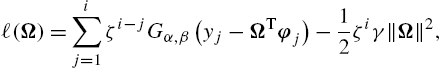
where ζ is the forgetting factor, satisfying 0≤ζ≤1![]() , γ is the regularization factor and Gα,β(yj−ΩTφj)=α2βΓ(1/α)exp(−|yj−ΩTφjβ|α)
, γ is the regularization factor and Gα,β(yj−ΩTφj)=α2βΓ(1/α)exp(−|yj−ΩTφjβ|α)![]() . Setting ∂∂Ωℓ(Ω)=0
. Setting ∂∂Ωℓ(Ω)=0![]() , one can obtain the solution
, one can obtain the solution
Ωi=(ΦiBiΦiT+γζiβαI)−1ΦiBiyi,
where
Bi=diag{b1,b2,…,bi}
with
bj=ζi−j×(yj−ΩTφj)α−2×(α22βΓ(1/α))×exp(−|yj−ΩTφjβ|α),j=1,2,…i.

With the matrix inversion lemma, we have
(ΦiBiΦiT+γζiβαI)−1ΦiBi=Φi(ΦiTΦi+γζiβαBi−1)−1.
Thus, (5.42) can be rewritten as
Ωi=Φi(ΦiTΦi+γζiβαBi−1)−1yi.
The above weight vector can be expressed as a linear combination of the transformed feature vectors, where the combination coefficients can be calculated recursively. We denote
Ωi=Φiai![]() with ai=(ΦiTΦi+γζiβαBi−1)−1yi
with ai=(ΦiTΦi+γζiβαBi−1)−1yi![]() being the coefficient vector. In addition, let Qi=(ΦiTΦi+γζiβα×Bi−1)−1
being the coefficient vector. In addition, let Qi=(ΦiTΦi+γζiβα×Bi−1)−1![]() . Then we have
. Then we have
Qi=[Φi−1TΦi−1+γζiβαBi−1−1Φi−1TφiφiTΦi−1φiTφi+γζiβαθi]−1,
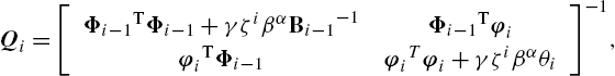
where θi=(yi−ΩTφi)α−2×(α22βΓ(1/α))×exp(−|yi−ΩTφiβ|α)![]() . The above result can be converted to
. The above result can be converted to
Qi−1=[Qi−1−1hihiTφiTφi+γζiβαθi],
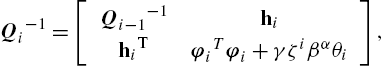
where hi=Φi−1Tφi![]() . Based on the following block matrix inversion identity,
. Based on the following block matrix inversion identity,
[ABCD]−1=[(A−BD−1C)−1−A−1B(D−CA−1B)−1−D−1C(A−BD−1C)−1(D−CA−1B)−1],
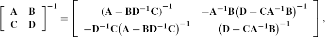
one can derive
Qi=ri−1[Qi−1ri+ziziT−zi−ziT1],
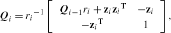
where ri=γζiβαθi+φiTφi−ziThi![]() and zi=Qi−1hi
and zi=Qi−1hi![]() . Therefore, the expansion coefficients are
. Therefore, the expansion coefficients are
ai=Qiyi=ri−1[Qi−1ri+ziziT−zi−ziT1][yi−1yi]=[ai−1−ziri−1eiri−1ei],
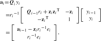
where ei=yi−ΩTφi![]() . Then we have obtained the GKRMC algorithm, whose pseudocode is given in Algorithm 4.
. Then we have obtained the GKRMC algorithm, whose pseudocode is given in Algorithm 4.
Remark
When α=2![]() , the GKRMC algorithm will reduce to the kernel recursive maximum correntropy (KRMC) developed in [38].
, the GKRMC algorithm will reduce to the kernel recursive maximum correntropy (KRMC) developed in [38].
5.5 Simulation Results
In the following, we present some simulation results to demonstrate the performance of the GKMC and GKRMC algorithms.
5.5.1 Frequency Doubling Problem
First, consider the frequency-doubling problem, where the input signal is a sine wave with 20 samples per period. The desired signal is another sine wave with double frequency, disturbed by an additive noise vi![]() . With a time embedding dimension of 5, the input vector is xi=[xi−4,xi−3,...,xi]
. With a time embedding dimension of 5, the input vector is xi=[xi−4,xi−3,...,xi]![]() . In this example, we consider a mixture noise model which combines two independent noise processes, given by
. In this example, we consider a mixture noise model which combines two independent noise processes, given by
vi=(1−δi)Ai+δiBi,
where δi![]() is binary distributed over {0,1}
is binary distributed over {0,1}![]() , with probability p(δi=1)=c
, with probability p(δi=1)=c![]() , p(δi=0)=1−c
, p(δi=0)=1−c![]() , where 0≤c≤1
, where 0≤c≤1![]() controls the occurrence probability of the noise processes Ai
controls the occurrence probability of the noise processes Ai![]() and Bi
and Bi![]() . In general, Ai
. In general, Ai![]() represents the “background noise” with small variance, while Bi
represents the “background noise” with small variance, while Bi![]() stands for large outliers that occur occasionally with larger variance. In the simulations below, without explicit mention we set c=0.05
stands for large outliers that occur occasionally with larger variance. In the simulations below, without explicit mention we set c=0.05![]() . Bi
. Bi![]() is assumed to be a white Gaussian process with zero mean and variance 15. The Gaussian kernel is adopted as the Mercer kernel in kernel adaptive filters and the bandwidth is set to σ=2.0
is assumed to be a white Gaussian process with zero mean and variance 15. The Gaussian kernel is adopted as the Mercer kernel in kernel adaptive filters and the bandwidth is set to σ=2.0![]() . The step sizes are chosen such that all the algorithms achieve almost the same initial convergence speed.
. The step sizes are chosen such that all the algorithms achieve almost the same initial convergence speed.
We choose 4000 noisy samples for training and 200 clean samples for testing (the filters are fixed during the testing). The average learning curves of the KLMS and GKMC over 100 Monte Carlo runs in terms of the testing MSEs with different values of α (λ=2.0![]() ) and distributions of Ai
) and distributions of Ai![]() (Gaussian and uniform) are illustrated in Fig. 5.3, and the corresponding testing MSEs at the final iteration are summarized in Table 5.1. From the simulation results we observe: (i) the GKMC can outperform the KLMS significantly, showing much stronger robustness with respect to the impulsive noises; (ii) with different values of α, the GKMC can achieve difference performances, and the best performance may be obtained when α≠2.0
(Gaussian and uniform) are illustrated in Fig. 5.3, and the corresponding testing MSEs at the final iteration are summarized in Table 5.1. From the simulation results we observe: (i) the GKMC can outperform the KLMS significantly, showing much stronger robustness with respect to the impulsive noises; (ii) with different values of α, the GKMC can achieve difference performances, and the best performance may be obtained when α≠2.0![]() . Note that the GKMC will reduce to the KMC algorithm when α=2.0
. Note that the GKMC will reduce to the KMC algorithm when α=2.0![]() .
.
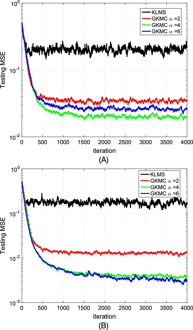
Table 5.1
Testing MSEs at final iteration in frequency doubling
| KLMS | GKMC α = 2 | GKMC α = 4 | GKMC α = 6 | |
|---|---|---|---|---|
| Gaussian | 0.2250 ± 0.1896 | 0.0353 ± 0.0168 | 0.0196 ± 0.0101 | 0.0260 ± 0.0121 |
| Uniform | 0.1781 ± 0.1842 | 0.0137 ± 0.0057 | 0.0037 ± 0.0016 | 0.0030 ± 0.0022 |

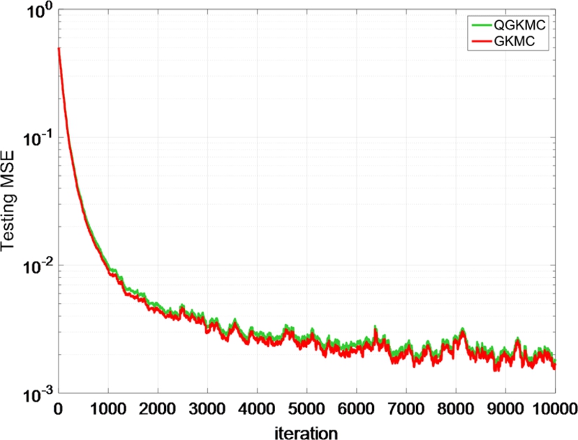
Further, we compare the performance of the GKMC and QGKMC. We set ε=0.03![]() , α=4
, α=4![]() , λ=2
, λ=2![]() and η=0.3
and η=0.3![]() and assume that Ai
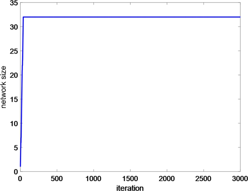
and assume that Ai![]() is of Gaussian distribution with variance 0.04. The average learning curves over 100 runs are shown in Fig. 5.4, and the network size growth curve of the QGKMC is presented in Fig. 5.5. One can see that both algorithms achieve almost the same convergence performance but the network size of QGKMC has been significantly curbed (only slightly larger than 30 at steady state).
is of Gaussian distribution with variance 0.04. The average learning curves over 100 runs are shown in Fig. 5.4, and the network size growth curve of the QGKMC is presented in Fig. 5.5. One can see that both algorithms achieve almost the same convergence performance but the network size of QGKMC has been significantly curbed (only slightly larger than 30 at steady state).
5.5.2 Online Nonlinear System Identification
Next, we show the performance of the GKMC and GKRMC algorithms in online nonlinear system identification. Suppose the nonlinear system is of the form [41]
yi=(0.8−0.5exp(−y2i−1))yi−1−(0.3+0.9exp(−y2i−1))yi−2+0.1sin(3.1415926yi−1)+vi,
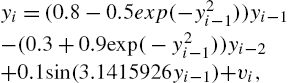
where vi![]() is a disturbance noise described by (5.50). The average learning curves in terms of testing MSEs over 100 Monte Carlo runs with different values of α and distributions of Ai
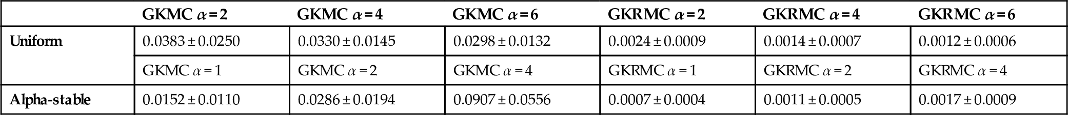
is a disturbance noise described by (5.50). The average learning curves in terms of testing MSEs over 100 Monte Carlo runs with different values of α and distributions of Ai![]() (uniform and alpha-stable) are shown in Fig. 5.6, and the corresponding testing MSEs at final iteration are listed in Table 5.2. In the simulation, 1000 noisy samples are used for training and 100 noise-free samples are used for testing (the filters are fixed during the testing). The parameters of the GKMC and GKRMC are experimentally chosen such that both achieve a desirable performance. It can be clearly seen that the GKRMC can outperform the GKMC, with faster convergence speed and lower testing MSE. However, we should note that the GKRMC is computationally more expensive than the GKMC.
(uniform and alpha-stable) are shown in Fig. 5.6, and the corresponding testing MSEs at final iteration are listed in Table 5.2. In the simulation, 1000 noisy samples are used for training and 100 noise-free samples are used for testing (the filters are fixed during the testing). The parameters of the GKMC and GKRMC are experimentally chosen such that both achieve a desirable performance. It can be clearly seen that the GKRMC can outperform the GKMC, with faster convergence speed and lower testing MSE. However, we should note that the GKRMC is computationally more expensive than the GKMC.
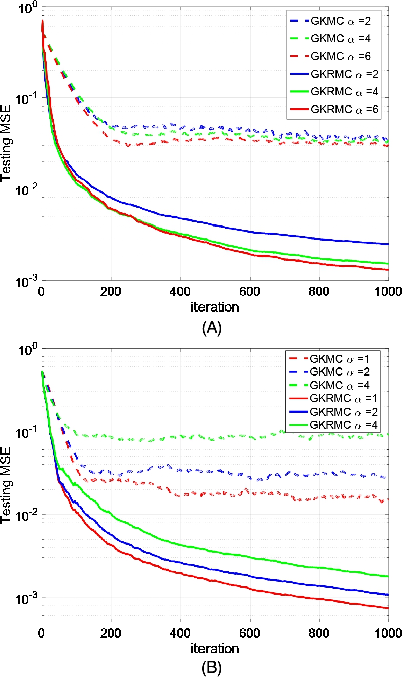
Table 5.2
Testing MSEs at the final iteration in online nonlinear system identification
| GKMC α = 2 | GKMC α = 4 | GKMC α = 6 | GKRMC α = 2 | GKRMC α = 4 | GKRMC α = 6 | |
|---|---|---|---|---|---|---|
| Uniform | 0.0383 ± 0.0250 | 0.0330 ± 0.0145 | 0.0298 ± 0.0132 | 0.0024 ± 0.0009 | 0.0014 ± 0.0007 | 0.0012 ± 0.0006 |
| GKMC α = 1 | GKMC α = 2 | GKMC α = 4 | GKRMC α = 1 | GKRMC α = 2 | GKRMC α = 4 | |
| Alpha-stable | 0.0152 ± 0.0110 | 0.0286 ± 0.0194 | 0.0907 ± 0.0556 | 0.0007 ± 0.0004 | 0.0011 ± 0.0005 | 0.0017 ± 0.0009 |
5.5.3 Noise Cancellation
In this part, we consider a noise cancellation problem in signal processing. The basic structure of a noise cancellation system is shown in Fig. 5.7. The primary signal is si![]() , whose noisy measurement di
, whose noisy measurement di![]() serves as the desired signal of the system. The term ρi
serves as the desired signal of the system. The term ρi![]() represents an unknown white noise process and xi
represents an unknown white noise process and xi![]() is its reference measurement. The signal xi
is its reference measurement. The signal xi![]() can be used as an input of an adaptive filter such that the filter output is an estimate of the noise ρi
can be used as an input of an adaptive filter such that the filter output is an estimate of the noise ρi![]() . Clearly, the signal-to-noise ratio (SNR) can be improved by subtracting the estimated noise from di
. Clearly, the signal-to-noise ratio (SNR) can be improved by subtracting the estimated noise from di![]() . In the simulation, the noise source is assumed to be uniformly distributed over [−0.5,0.5]
. In the simulation, the noise source is assumed to be uniformly distributed over [−0.5,0.5]![]() . The interference distortion function is
. The interference distortion function is
xi=ρi−0.2xi−1−xi−1ρi−1+0.1ρi−1+0.4xi−2,
which is nonlinear with an infinite impulsive response. It is impossible to recover ρi![]() from a finite time delay embedding of xi
from a finite time delay embedding of xi![]() . Actually, one can rewrite the distortion function as
. Actually, one can rewrite the distortion function as
ρi=xi+0.2xi−1−0.4xi−2+(xi−1−0.1)ρi−1.
Obviously, the present value of the noise source ρi![]() not only depends on the reference noise measurements [xi,xi−1,xi−2]
not only depends on the reference noise measurements [xi,xi−1,xi−2]![]() , but also on the past value ρi−1
, but also on the past value ρi−1![]() . However, the filter output yi−1
. However, the filter output yi−1![]() can be used as a surrogate signal. In this case, the input vector of the adaptive filter is [xi,xi−1,xi−2,yi−1]
can be used as a surrogate signal. In this case, the input vector of the adaptive filter is [xi,xi−1,xi−2,yi−1]![]() . We assume the primary signal si=0
. We assume the primary signal si=0![]() during the training phase. The system tries to reconstruct the noise source from the reference measurements. We use three nonlinear filters trained with KLMS, KRLS and GKRMC, respectively. In the simulation, the step size and the Gaussian kernel bandwidth for KLMS are 2.0 and 0.15. The regularization parameter for KRLS and GKRMC is 0.1. The Gaussian kernel bandwidth for KRLS and GKRMC are 0.17 and 0.1, respectively. The parameter β for GKRMC is set to 0.5. The ensemble learning curves over 100 Monte Carlo runs for different algorithms are illustrated in Fig. 5.8. In addition, the noise reduction factor (NR) defined by 10log10{E[ρ2i]/E[ρi−yi]2}
during the training phase. The system tries to reconstruct the noise source from the reference measurements. We use three nonlinear filters trained with KLMS, KRLS and GKRMC, respectively. In the simulation, the step size and the Gaussian kernel bandwidth for KLMS are 2.0 and 0.15. The regularization parameter for KRLS and GKRMC is 0.1. The Gaussian kernel bandwidth for KRLS and GKRMC are 0.17 and 0.1, respectively. The parameter β for GKRMC is set to 0.5. The ensemble learning curves over 100 Monte Carlo runs for different algorithms are illustrated in Fig. 5.8. In addition, the noise reduction factor (NR) defined by 10log10{E[ρ2i]/E[ρi−yi]2}![]() is given in Table 5.3. In this example, the GKRMC achieves the best performance when α=6
is given in Table 5.3. In this example, the GKRMC achieves the best performance when α=6![]() .
.
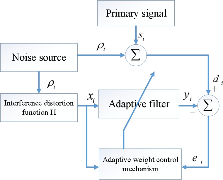
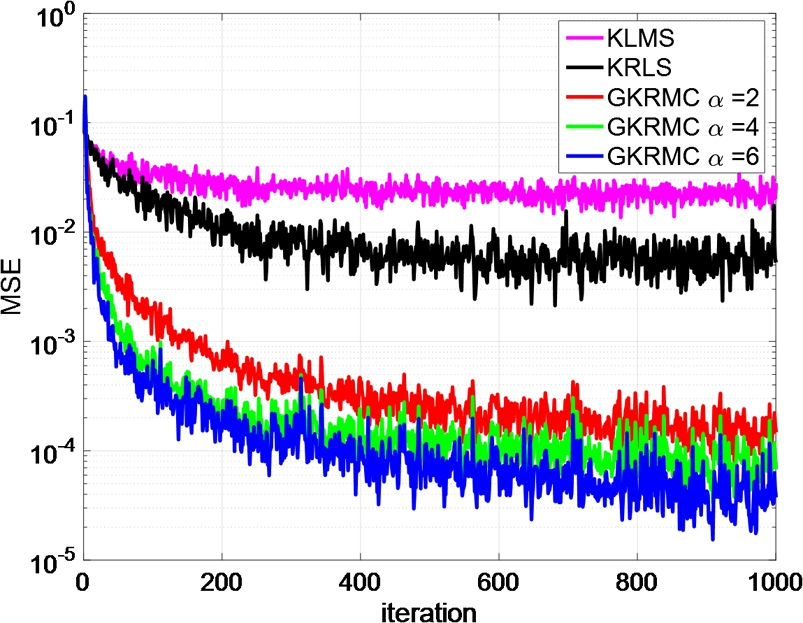
Table 5.3
Performance comparison of KLMS, KRLS and GKRMC in noise cancellation
| Algorithm | KLMS | KRLS | GKMC α = 2 | GKMC α = 4 | GKMC α = 6 |
|---|---|---|---|---|---|
| NR (dB) | 5.7356 ± 0.6441 | 11.6057 ± 1.3710 | 27.4908 ± 1.2422 | 30.5206 ± 1.4516 | 33.5343 ± 1.7440 |

5.6 Conclusion
In this chapter, we characterized a unified and efficient approach to deal with online nonlinear modeling with non-Gaussian noises, which combines the powerful modeling capability of the KAFs and the robustness of the MCC with respect to heavy-tailed non-Gaussian noises. We focused mainly on the KLMS- and KRLS-type algorithms but the results can easily be extended to other KAFs. Particularly the GKMC and GKRMC algorithms were presented. Simulation results on frequency doubling, nonlinear system identification and noise cancellation have been presented to illustrate the benefits of the new approach.