
A Random Fourier Features Perspective of KAFs With Application to Distributed Learning Over Networks
Pantelis Bouboulis⁎; Sergios Theodoridis⁎; Symeon Chouvardas† ⁎National and Kapodistrian University of Athens, Athens, Greece
†Capital Fund Management, Paris, France
Abstract
A major problem in any typical online kernel-based scheme is that the model's solution is given as an expansion of kernel functions that grows linearly with time. Usually, some sort of pruning strategy is adopted to make the solution sparse for practical reasons. The key idea is to keep the most informative training data in the expansion (the so-called dictionary), while the rest is omitted. Although these strategies have been proven effective, they still consume computational resources due to their nature (e.g., they require a sequential search of the dictionary at each time instant) and they limit the design of kernel-based methods in more general settings, as for example in distributed systems. In this chapter, we show how one can employ random features of the kernel function to transform the original nonlinear problem, which lies in an infinite-dimensional Hilbert space, to a fixed-dimension Euclidean space, without significantly compromising performance. This paves the way for designing kernel-based methods for distributed systems based on their linear counterparts.
Keywords
Online kernel-based learning; Online distributed kernel-based learning; Random Fourier features
Chapter Points
- • Provide an overview of the random Fourier features rationale, as a tool to approximate the kernel.
- • Provide a review of existing online kernel-based schemes (e.g., KLMS, KRLS, PEGASOS), using the random Fourier features procedure.
- • Propose elegant and efficient online distributed kernel-based schemes for learning over networks, using the random Fourier features rationale.
7.1 Introduction
During the last decade, there has been an increasing interest for online learning schemes based on the rationale of reproducing kernels both for regression and classification. This has been sparked by the great success of the Support Vectors Machines (SVMs) and other related kernel methods [1–3] in addressing nonlinear tasks in a batch setting. Similar to the way that the kernel trick generalizes the classical linear SVM to the nonlinear case, these methods exploit the inner product structure of a Reproducing Kernel Hilbert Space (RKHS), H![]() , to modify well-established linear learning methods (such as the LMS and the RLS) to treat nonlinear tasks [4–7]. In essence, the data are transformed to a high-dimensional space equipped with an inner product (induced by the selected kernel) and then standard linear learning methods are applied to the transformed data. This is equivalent to nonlinear processing in the original space.
, to modify well-established linear learning methods (such as the LMS and the RLS) to treat nonlinear tasks [4–7]. In essence, the data are transformed to a high-dimensional space equipped with an inner product (induced by the selected kernel) and then standard linear learning methods are applied to the transformed data. This is equivalent to nonlinear processing in the original space.
In general, these methods consider that the training data points {(xn,y(n)),n=1,2,…}![]() , xn∈Rd
, xn∈Rd![]() , are generated by a nonlinear model of the form y=g(x)
, are generated by a nonlinear model of the form y=g(x)![]() , where g is an unknown nonlinear function, and that the data pairs arrive in a sequential (online) fashion. The objective is to learn a function f∈H
, where g is an unknown nonlinear function, and that the data pairs arrive in a sequential (online) fashion. The objective is to learn a function f∈H![]() , to minimize a certain cost, i.e., L(xn,y(n),f)
, to minimize a certain cost, i.e., L(xn,y(n),f)![]() . Typically, a specific kernel function, κ, is selected and each data pair (arriving at the nth time instant) is mapped to (Φ(xn),y(n))
. Typically, a specific kernel function, κ, is selected and each data pair (arriving at the nth time instant) is mapped to (Φ(xn),y(n))![]() , using the feature map Φ:Rd→H:Φ(x)=κ(x,⋅)
, using the feature map Φ:Rd→H:Φ(x)=κ(x,⋅)![]() . Consequently, the system's output is modeled as 〈Φ(xn),f〉H
. Consequently, the system's output is modeled as 〈Φ(xn),f〉H![]() and the data pair is used to update the previously available estimate of f. The result is that (after n iterations) the solution, at time instant n, is given in terms of all past training points, i.e.,
and the data pair is used to update the previously available estimate of f. The result is that (after n iterations) the solution, at time instant n, is given in terms of all past training points, i.e.,
fn=n∑i=1wiΦ(xi)=n∑i=1wiκ(xi,⋅).
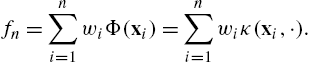
Since n can grow indefinitely, it is evident that this scheme soon becomes impractical. This becomes very serious in big data applications, where online algorithms are the only viable possibility, e.g., [3]. Usually, some sort of pruning criterion is adopted to make the aforementioned linear expansion sparse. Thus, a dictionary is formed, which contains all valid training points (centers and coefficients) and the specific criterion is used to determine whether a new point will enter the dictionary or not. For example, if the novelty criterion is adopted, new arriving points enter the expansion only if the respective center, xn![]() , is far away from all other centers of the dictionary. If the quantization criterion is adopted, the centers are quantized and each new data pair is used to update the coefficient of the dictionary's center with the same quantization value.
, is far away from all other centers of the dictionary. If the quantization criterion is adopted, the centers are quantized and each new data pair is used to update the coefficient of the dictionary's center with the same quantization value.
In this chapter, we propose a different approach. Based on the original idea of Rahimi and Recht [8], which has also been applied in [9,10] in a similar context, we approximate the kernel function using randomly selected Fourier features and transform the problem from the original RKHS, H![]() , to another Euclidean space RD
, to another Euclidean space RD![]() . Thus, we can model the solution as a fixed-size vector in RD
. Thus, we can model the solution as a fixed-size vector in RD![]() and directly apply any desired linear learning method. More importantly, we can use this rationale to develop learning methods over distributed networks. These are decentralized networks, which are represented by different nodes; each node collects the observations in a sequential fashion and communicates with a subset of nodes, which define its neighborhood, in order to reach a consensus regarding the solution. In such a setting, although the noise and observations, in each node, may follow different statistics, the parameters defining the generating model are assumed to be common for all nodes. The problem in this case is that, if one follows the rationale of Eq. (7.1), the typical sparsification methods become increasingly complicated, as each node has to transmit the entire sum at each time instant to its neighbors and the node has to, somehow, fuse together all received sums to compute the updated estimate. This is probably the reason that (until now) no practical solutions for online learning with kernels in distributed networks have been proposed. On the contrary, we will show that the newly proposed scheme can be directly applied to distributed environments and that the standard established linear methods can be exploited.
and directly apply any desired linear learning method. More importantly, we can use this rationale to develop learning methods over distributed networks. These are decentralized networks, which are represented by different nodes; each node collects the observations in a sequential fashion and communicates with a subset of nodes, which define its neighborhood, in order to reach a consensus regarding the solution. In such a setting, although the noise and observations, in each node, may follow different statistics, the parameters defining the generating model are assumed to be common for all nodes. The problem in this case is that, if one follows the rationale of Eq. (7.1), the typical sparsification methods become increasingly complicated, as each node has to transmit the entire sum at each time instant to its neighbors and the node has to, somehow, fuse together all received sums to compute the updated estimate. This is probably the reason that (until now) no practical solutions for online learning with kernels in distributed networks have been proposed. On the contrary, we will show that the newly proposed scheme can be directly applied to distributed environments and that the standard established linear methods can be exploited.
The rest of the chapter is organized as follows. Section 7.2 presents the kernel approximation rationale of Rahimi and Recht. In Section 7.3, it is shown how the aforementioned kernel approximation rationale can be exploited to generate fixed-budget kernel-based online learning methods (kernel adaptive filters). The section contains fixed-budget implementations of the KLMS, the KRLS and the kernel-PEGASOS algorithms, as well as simulations to demonstrate the effectiveness of the methods. Moreover, in Section 7.4 the kernel approximation rationale is employed to generate elegant and efficient distributed learning methods over networks, based on the combine-then-adapt strategy. Finally, Section 7.5 presents some concluding remarks.
7.2 Approximating the Kernel
All kernel-based learning techniques usually demand a large number of kernel computations between training samples. For example, the popular SVM algorithm requires the computation of a large kernel matrix consisting of the kernel evaluations between pairs of all possible combinations of the training points. Hence, to alleviate the computational burden, one common line of research suggests to use some sort of approximation of the kernel matrix. This can be done by the celebrated Nyström method [11,12] or by other similar techniques. In this chapter, we are focusing on the Fourier features approach proposed in [8,13], as this fits more naturally to the online setting. The following theorem plays a key role in this procedure.
Theorem 1
Consider a shift-invariant positive definite kernel κ(x−y)![]() defined on Rd
defined on Rd![]() and its Fourier transform, p(ω)=1(2π)d∫Rdκ(δ)e−iωTδdδ
and its Fourier transform, p(ω)=1(2π)d∫Rdκ(δ)e−iωTδdδ![]() , which (according to Bochner's theorem) can be regarded as a probability density function. Then, defining zω,b(x)=√2cos(ωTx+b)
, which (according to Bochner's theorem) can be regarded as a probability density function. Then, defining zω,b(x)=√2cos(ωTx+b)![]() , it turns out that
, it turns out that
κ(x−y)=Eω,b[zω,b(x)zω,b(y)],
where ω is drawn from p, b from the uniform distribution on [0,2π]![]() and E[⋅]
and E[⋅]![]() denotes the related expectation.
denotes the related expectation.
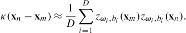
Following Theorem 1, we choose to approximate κ(xn−xm)![]() using D random Fourier features, ω1,ω2,…,ωD
using D random Fourier features, ω1,ω2,…,ωD![]() , (drawn from p) and D random numbers, b1,b2,…,bD
, (drawn from p) and D random numbers, b1,b2,…,bD![]() (drawn uniformly from [0,2π]
(drawn uniformly from [0,2π]![]() ) that define a sample average:
) that define a sample average:
κ(xn−xm)≈1DD∑i=1zωi,bi(xm)zωi,bi(xn).
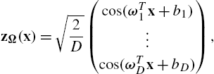
Hence, instead of relying on the implicit map, Φ, provided by the kernel trick, we can map the input data to a finite-dimensional Euclidean space (with dimension lower than H![]() , but still larger than the input space) using the randomized feature map zΩ:Rd→RD
, but still larger than the input space) using the randomized feature map zΩ:Rd→RD![]() :
:
zΩ(x)=√2D(cos(ωT1x+b1)⋮cos(ωTDx+bD)),
where Ω is the (d+1)×D![]() matrix defining the random Fourier features of the respective kernel, i.e.,
matrix defining the random Fourier features of the respective kernel, i.e.,
Ω=(ω1ω2...ωDb1b2...bD),
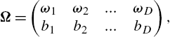
so that the kernel evaluations can be approximated as κ(xn,xm)≈zΩ(xn)TzΩ(xm)![]() . Details on the quality of this approximation, as well as other theoretical results, can be found in [8,13–15]. We note that for the Gaussian kernel, i.e., κσ(x,y)=exp(−‖x−y‖2/σ2)
. Details on the quality of this approximation, as well as other theoretical results, can be found in [8,13–15]. We note that for the Gaussian kernel, i.e., κσ(x,y)=exp(−‖x−y‖2/σ2)![]() , which is employed throughout the paper, the respective Fourier transform becomes
, which is employed throughout the paper, the respective Fourier transform becomes
p(ω)=(σ/√2π)De−σ2‖ω‖22,
which is actually the multivariate Gaussian distribution with mean 0D![]() and covariance matrix 1σ2ID
and covariance matrix 1σ2ID![]() .
.
7.3 Online Kernel-Based Learning: A Random Fourier Features Perspective
Inspired by the randomized feature map, we propose an alternative approach for online learning in RKHS. The procedure can be summarized as follows:
- • Map all data pairs, to (zΩ(xn),y(n))
 .
. - • Approximate the desired output as f(x)≈θTzΩ(x)
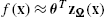 , for some θ∈RD
 .
. - • Estimate θ using any standard linear learning method (e.g., LMS, RLS) on the transformed data.
In the following, we will demonstrate in details three applications of the proposed procedure: (a) the Kernel LMS (KLMS), (b) the Kernel RLS (KRLS) and (c) the Primal Estimated sub-GrAdient SOlver for non linear SVM (kernel PEGASOS).
7.3.1 RFF-KLMS
Assuming a sequentially arriving data set, {(zΩ(xn),y(n)),n=1,2,…}![]() , the typical LMS algorithm models the desired output as f(x)=ˆy=θTzΩ(x)
, the typical LMS algorithm models the desired output as f(x)=ˆy=θTzΩ(x)![]() and estimates θ, so that the MSE cost function, L(xn,y(n),θ)=E[(y(n)−θTzΩ(xn))2]
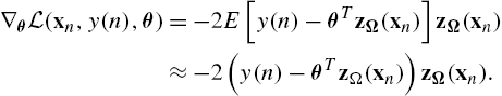
and estimates θ, so that the MSE cost function, L(xn,y(n),θ)=E[(y(n)−θTzΩ(xn))2]![]() is minimized. The minimization is carried out via a gradient descent rationale, where the gradient of the cost, is approximated by the current measurement, i.e.,
is minimized. The minimization is carried out via a gradient descent rationale, where the gradient of the cost, is approximated by the current measurement, i.e.,
∇θL(xn,y(n),θ)=−2E[y(n)−θTzΩ(xn)]zΩ(xn)≈−2(y(n)−θTzΩ(xn))zΩ(xn).
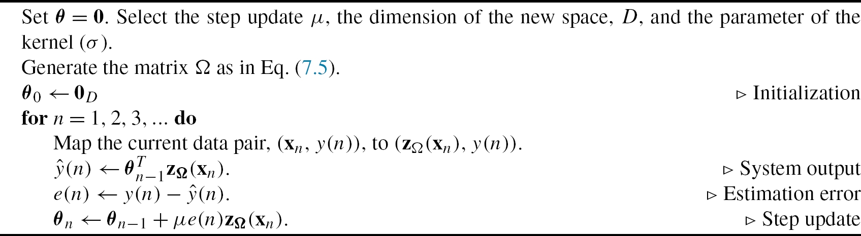
This method (RFF-KLMS) has been introduced independently in [9] and [10]. Algorithm 1 presents the steps in details. It is a matter of elementary algebra to see that after n−1![]() steps, the estimation of the solution will be θn=μ∑n−1i=1e(i)zΩ(xi)
steps, the estimation of the solution will be θn=μ∑n−1i=1e(i)zΩ(xi)![]() , which leads us to conclude that the RFF-KLMS scheme will produce, approximately, the same output as that of the standard KLMS (provided that D is sufficiently large):
, which leads us to conclude that the RFF-KLMS scheme will produce, approximately, the same output as that of the standard KLMS (provided that D is sufficiently large):
ˆy(n)=μn−1∑i=1e(i)zΩ(xi)TzΩ(xn)≈μn−1∑i=1e(i)κ(xi,xn),
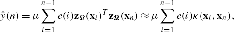
where for the last relation (which gives the output of the standard KLMS [7,4]) we used Theorem 1. The major difference is that the RFF-KLMS provides a single vector θ of fixed dimensions, instead of a growing expansion of kernel functions, hence no pruning mechanisms are required.
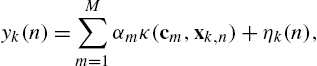
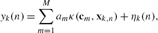
Working similar to the case of the standard LMS, we can study convergence properties of RFFKLMS. Henceforth, we will assume that the data pairs are generated by
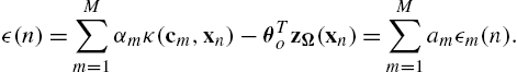
y(n)=M∑m=1αmκ(cm,xn)+η(n),

where c1,…,cM![]() are fixed centers, xn
are fixed centers, xn![]() are zero-mean independent and identically distributed samples drawn from the Gaussian distribution with covariance matrix σ2XId
are zero-mean independent and identically distributed samples drawn from the Gaussian distribution with covariance matrix σ2XId![]() and η(n)
and η(n)![]() are independent and identically distributed noise samples drawn from N(0,σ2η)
are independent and identically distributed noise samples drawn from N(0,σ2η)![]() . We note that the parameters σX
. We note that the parameters σX![]() and ση
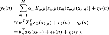
and ση![]() are the variances of the input and the noise, respectively, and they are not in any way related to the kernel parameter σ. Applying the approximation rationale of Theorem 1, we obtain
are the variances of the input and the noise, respectively, and they are not in any way related to the kernel parameter σ. Applying the approximation rationale of Theorem 1, we obtain
κ(cm,xn)=Eω,b[zω,b(cm)zω,b(xn)]=zΩ(cm)TzΩ(xn)+ϵm(n),
where ϵm(n)![]() is the error between the actual value of the kernel function and the approximated one. Thus, if we define
is the error between the actual value of the kernel function and the approximated one. Thus, if we define
ZC=(zΩ(c1),…,zΩ(cM)),α=(α1,…,αM)T,θo=ZΩα,
we get
y(n)=αTZTΩzΩ(xn)+ϵ(n)+η(n)=θTozΩ(xn)+ϵ(n)+η(n),
where ϵ(n)![]() stands for the approximation error between the noise-free component of y(n)
stands for the approximation error between the noise-free component of y(n)![]() (evaluated only by the linear kernel expansion of Eq. (7.8)) and the approximation of this component using random Fourier features, i.e.,
(evaluated only by the linear kernel expansion of Eq. (7.8)) and the approximation of this component using random Fourier features, i.e.,
ϵ(n)=M∑m=1αmκ(cm,xn)−θTozΩ(xn)=M∑m=1amϵm(n).
Let x∈Rd![]() , y∈R
, y∈R![]() , be the random variables that generate the measurements and Rzz=E[zΩ(x)zTΩ(x)]
, be the random variables that generate the measurements and Rzz=E[zΩ(x)zTΩ(x)]![]() the corresponding autocorrelation matrix. We can prove that Rzz
the corresponding autocorrelation matrix. We can prove that Rzz![]() is positive definite, provided that all the random features are different from each other, i.e., ωi≠ωj
is positive definite, provided that all the random features are different from each other, i.e., ωi≠ωj![]() , for all i≠j
, for all i≠j![]() [16]. Thus, the cross-correlation vector takes the form
[16]. Thus, the cross-correlation vector takes the form
E[zΩ(x)y]=E[zΩ(x)(zΩ(x)Tθo+ϵ+η)]=Rzzθo+E[zΩ(x)ϵ],
where for the last relation we have used the fact that η is a zero-mean variable representing noise and that zΩ(x)![]() and η are independent. For large enough D, we can assume that the approximation error, ϵ, approaches 0 [14], hence the optimal solution becomes
and η are independent. For large enough D, we can assume that the approximation error, ϵ, approaches 0 [14], hence the optimal solution becomes
θ⁎=E[(y−zΩ(x)Tθo)2]=R−1zz(Rzzθo+E[zΩ(x)ϵ])=θo+R−1zzE[zΩ(x)ϵ]≈θo.

To summarize, the proposed rationale assumes that, for sufficiently large D, Eq. (7.8) can be closely approximated by y(n)≈αTZTCzΩ(xn)+η(n)![]() . The major difference with the standard LMS case is that the transformed inputs, zΩ(xn)
. The major difference with the standard LMS case is that the transformed inputs, zΩ(xn)![]() , can no longer be assumed to be generated by the Gaussian distribution. Applying similar assumptions as in the case of the standard LMS (e.g., independence between xn,xm
, can no longer be assumed to be generated by the Gaussian distribution. Applying similar assumptions as in the case of the standard LMS (e.g., independence between xn,xm![]() , for n≠m
, for n≠m![]() and between xn,η(n)
and between xn,η(n)![]() ), we get several convergence properties, where the eigenvalues of the positive definite matrix Rzz
), we get several convergence properties, where the eigenvalues of the positive definite matrix Rzz![]() , i.e., 0<λ1⩽λ2⩽⋯⩽λD
, i.e., 0<λ1⩽λ2⩽⋯⩽λD![]() , play a pivotal role:
, play a pivotal role:
- 1. If 0<μ<2/λD
 , then RFFKLMS converges in the mean, i.e., E[θn−θo]→0
 .
. - 2. The optimal MSE is given by
J(n)opt=σ2η+E[ϵ(n)]−E[ϵ(n)zΩ(xn)]R−1zzE[ϵ(n)zΩ(xn)T].
- For large enough D, we have J(n)opt≈σ2η
 .
. - 3. The excess MSE is given by J(n)ex=J(n)−J(n)opt=tr(RzzAn)
 , where An=E[(θn−θo)(θn−θo)T]
 .
. - 4. If 0<μ<1/λD
 , then An
 converges.
7.3.2 RFF-KRLS
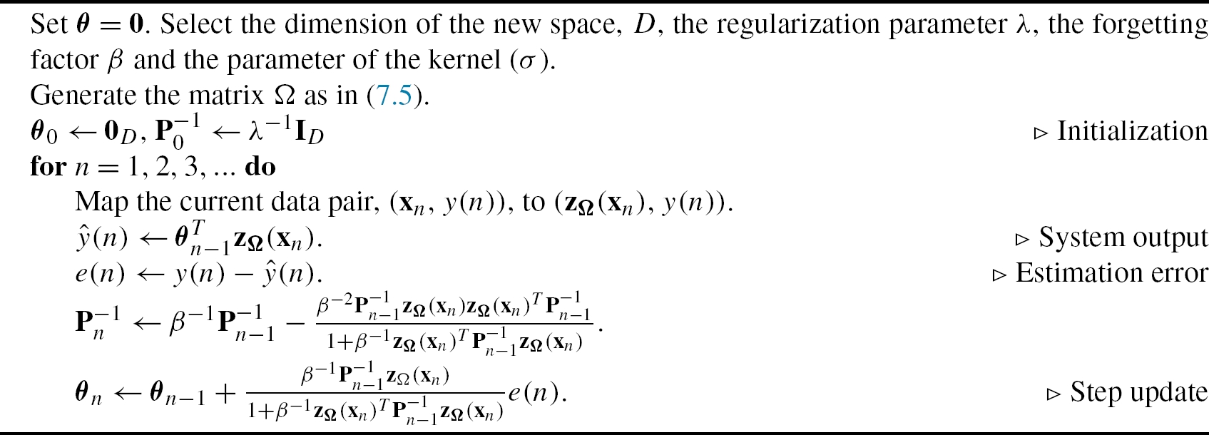
Contrary to the stochastic approach employed by the LMS, the RLS utilizes information of all past data to estimate θ by minimizing the regularized risk cost function, i.e.,
L(xn,y(n),θ)=n∑k=1βn−k(y(n)−θTzΩ(xn))2+λβn‖θ‖2,
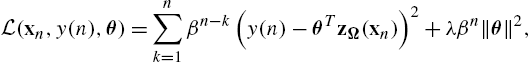
for some chosen λ>0![]() , where β is a weighting factor that is usually added as a forgetting mechanism and which makes the algorithm more sensitive to recent data. Solving θ⁎=minθL(xn,y(n),θ)
, where β is a weighting factor that is usually added as a forgetting mechanism and which makes the algorithm more sensitive to recent data. Solving θ⁎=minθL(xn,y(n),θ)![]() requires the inversion of an n×n
requires the inversion of an n×n![]() matrix at each step. However, employing the matrix inversion lemma, it is possible to compute this solution recursively. Algorithm 2 presents the details. The procedure is identical to that of the standard RLS, except that we replace xn
matrix at each step. However, employing the matrix inversion lemma, it is possible to compute this solution recursively. Algorithm 2 presents the details. The procedure is identical to that of the standard RLS, except that we replace xn![]() with the transformed data zΩ(xn)
with the transformed data zΩ(xn)![]() . Moreover, we should note that, unlike the LMS case, the proposed scheme provides a solution that is different from other implementations of KRLS (like the ones presented in [6] and [4]). Although all KRLS-like implementations, provided in the respective literature, estimate the system's output as a linear expansion of kernel functions centered at the past data, the estimation of the expansion's coefficients differs in the case presented here.
. Moreover, we should note that, unlike the LMS case, the proposed scheme provides a solution that is different from other implementations of KRLS (like the ones presented in [6] and [4]). Although all KRLS-like implementations, provided in the respective literature, estimate the system's output as a linear expansion of kernel functions centered at the past data, the estimation of the expansion's coefficients differs in the case presented here.
7.3.3 RFF-PEGASOS
The methods presented in Sections 7.3.1 and 7.3.2 are suitable for online regression problems. In this section, we present an online classification method based on the PEGASOS scheme (see [17]). Consider a training set of the form {(xn,y(n)),n=1,2,…N}![]() , where xn∈Rd
, where xn∈Rd![]() and y(n)=±1
and y(n)=±1![]() . PEGASOS is an SVM-like algorithm that processes the data sequentially as follows. On iteration t, the algorithm selects a random training example (xnt,y(nt))
. PEGASOS is an SVM-like algorithm that processes the data sequentially as follows. On iteration t, the algorithm selects a random training example (xnt,y(nt))![]() by picking an index nt
by picking an index nt![]() uniformly at random from {1,2,…,N}
uniformly at random from {1,2,…,N}![]() . The scheme follows a stochastic gradient rationale, adopting the regularized hinge loss function, i.e.,
. The scheme follows a stochastic gradient rationale, adopting the regularized hinge loss function, i.e.,
θ⁎=max{0,1−y〈f,Φ(x)〉H}+λ2‖f‖2H,
where H![]() is the RKHS associated with a preselected kernel κ and Φ the respective feature map. Thus, the step update equation becomes:
is the RKHS associated with a preselected kernel κ and Φ the respective feature map. Thus, the step update equation becomes:
ft=(1−1t)ft−1+1+(1−y(nt)〈ft−1,Φ(xnt)〉H)yntλtΦ(xnt).

After a predetermined number of iterations (say T), the algorithm provides the solution, which is given as a sparse linear expansion of kernel functions, similar to Eq. (7.1). The algorithm is implemented by keeping in memory an N-size vector that comprises all the coefficients of the expansion. During each iteration, at most one of these coefficients might change. The performance of the scheme has been shown to improve with data reuse, i.e., when the same data are used again and again for training.
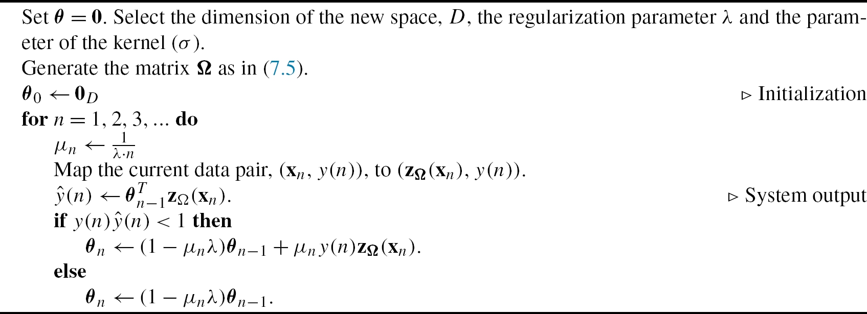
Evidently, since the solution provided by the algorithm depends on the dataset's size, PEGASOS cannot be considered as an online scheme (where the actual size of the dataset is not known beforehand). However, employing the random Fourier features rationale, we can model the output as f(x)=θTzΩ(x)![]() , where θ∈RD
, where θ∈RD![]() , and thus rewrite the step update equation as follows (see Algorithm 3):
, and thus rewrite the step update equation as follows (see Algorithm 3):
θn=(1−1n)θn−1+1+(1−y(n)θTn−1zΩ(xn))y(n)λnzΩ(xn),

where we have assumed that the data arrive sequentially. Similar to the LMS case, the proposed algorithm can be seen as a linear PEGASOS on the dataset {(zΩ(xn),y(n)),n=1,2,…}![]() , hence all convergence properties of [17] hold in this case too. We will call this scheme RFF-PEGASOS.
, hence all convergence properties of [17] hold in this case too. We will call this scheme RFF-PEGASOS.
We should note that the proposed algorithm features several significant advantages with respect to the original form of kernel PEGASOS presented in [17]. Firstly, the complexity per iteration is O(Dd)![]() and does not depend on the training database size, in contrast with the kernel-PEGASOS, which has complexity O(Md)
and does not depend on the training database size, in contrast with the kernel-PEGASOS, which has complexity O(Md)![]() , M being the number of the support vectors. Moreover, RFF-PEGASOS solves the problem of the growing sum and thus it can work in a truly online fashion (where the dataset is not known beforehand), while kernel-PEGASOS was designed for batch processing (i.e., fixed datasets). Finally, it is evident that for datasets with many support vectors (where M>>D
, M being the number of the support vectors. Moreover, RFF-PEGASOS solves the problem of the growing sum and thus it can work in a truly online fashion (where the dataset is not known beforehand), while kernel-PEGASOS was designed for batch processing (i.e., fixed datasets). Finally, it is evident that for datasets with many support vectors (where M>>D![]() ) RFF-PEGASOS is significantly faster. However, in databases with a low number of support vectors (M<<D
) RFF-PEGASOS is significantly faster. However, in databases with a low number of support vectors (M<<D![]() ), it runs slower.
), it runs slower.
7.3.4 Simulations—Regression
In this section, we provide some simple simulations, which are indicative of the behavior of the proposed algorithms, compared to their typical implementations. For the regression case, we generate 5000 data pairs using the following model: y(n)=∑Mm=1amκ(cm,xn)+η(n)![]() , where xn∈R5
, where xn∈R5![]() are drawn from N(0,I5)
are drawn from N(0,I5)![]() and the noise are independent and identically distributed Gaussian samples with ση=0.1
and the noise are independent and identically distributed Gaussian samples with ση=0.1![]() . The parameters of the expansion (i.e., a1,…,aM
. The parameters of the expansion (i.e., a1,…,aM![]() ) are drawn from N(0,25)
) are drawn from N(0,25)![]() and the kernel parameter σ is set to 5. The specific parameters of the algorithms are shown in Table 7.1. We compare RFF-KLMS and RFF-KRLS with a standard implementation of KLMS using the quantization pruning technique and the KRLS version of [6]. Fig. 7.1 shows the evolution of the MSE for 100 realizations of the experiment for several values of D (i.e., the total number of random Fourier features used), where the number of the free parameters of the model is set to M=100
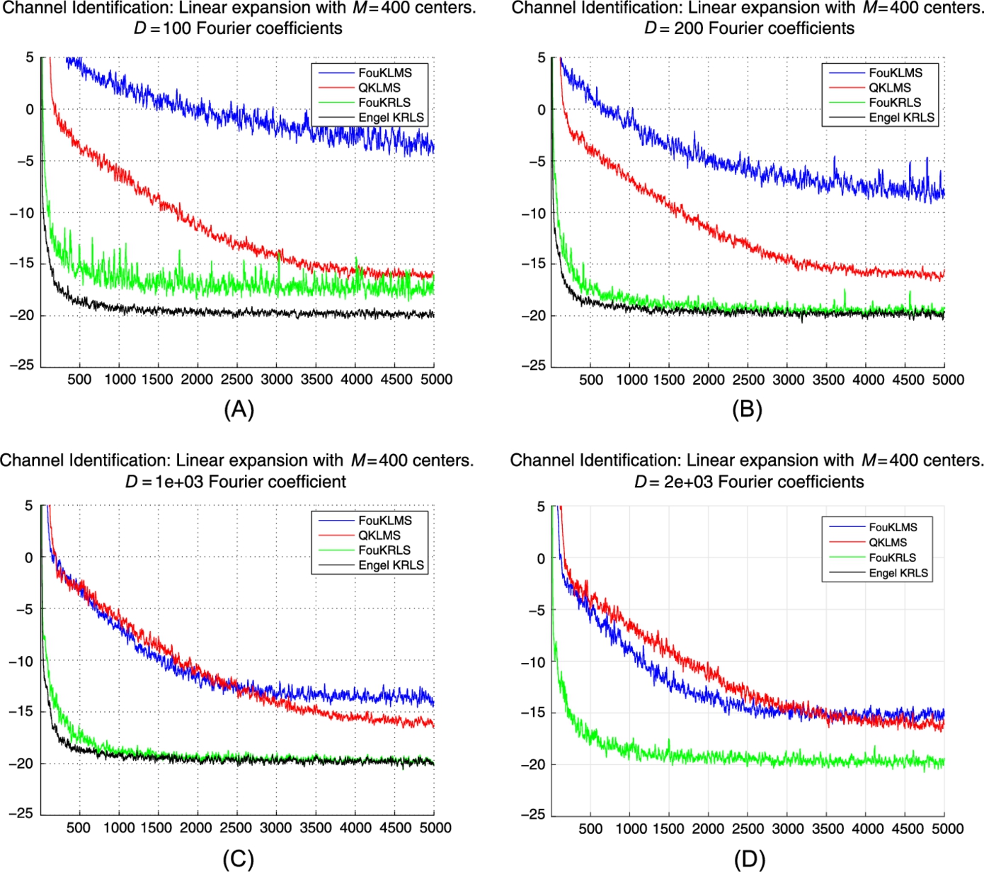
and the kernel parameter σ is set to 5. The specific parameters of the algorithms are shown in Table 7.1. We compare RFF-KLMS and RFF-KRLS with a standard implementation of KLMS using the quantization pruning technique and the KRLS version of [6]. Fig. 7.1 shows the evolution of the MSE for 100 realizations of the experiment for several values of D (i.e., the total number of random Fourier features used), where the number of the free parameters of the model is set to M=100![]() . As this is a kernel approximation scheme, it is expected that the performance (in terms of MSE) would be somewhat reduced. However, we can see in Fig. 7.1 that the performance of both RFF-KLMS and RFF-KRLS is very close to their typical implementations. In this particular example, both algorithms can achieve similar performance with their standard counterparts earlier in time (see Table 7.2 and Figs. 7.1B, 7.1D for the KLMS and KRLS, respectively). Fig. 7.2 shows the evolution of the MSE for the same experiment using M=400
. As this is a kernel approximation scheme, it is expected that the performance (in terms of MSE) would be somewhat reduced. However, we can see in Fig. 7.1 that the performance of both RFF-KLMS and RFF-KRLS is very close to their typical implementations. In this particular example, both algorithms can achieve similar performance with their standard counterparts earlier in time (see Table 7.2 and Figs. 7.1B, 7.1D for the KLMS and KRLS, respectively). Fig. 7.2 shows the evolution of the MSE for the same experiment using M=400![]() parameters in the design model. In this case, it is evident that a larger number of Fourier features is required to achieve the same approximation quality. For example, the RFF-KRLS requires more than D=200
parameters in the design model. In this case, it is evident that a larger number of Fourier features is required to achieve the same approximation quality. For example, the RFF-KRLS requires more than D=200![]() random features and the RFF-KLMS requires D=2000
random features and the RFF-KLMS requires D=2000![]() features to achieve approximately the same steady-state MSE as their typical variants. To conclude:
features to achieve approximately the same steady-state MSE as their typical variants. To conclude:
- • Both RFF-KLMS and RFF-KRLS can efficiently approximate their typical counterparts for large enough values of D>D0
 .
. - • The value of D needed (so that the RFF-KLMS and the KRLS approximate their counterparts) depends on the model complexity (it also depends on the size of the input space, d, for obvious reasons).
- • The RFF-KRLS can achieve the same performance with the KRLS using significantly smaller D than the one needed by the RFF-KLMS for comparable performance to KLMS. Possibly, this is due to the fact that the KRLS mechanism utilizes all past data in each iteration.
Table 7.1
The parameters of the KLMS and KRLS variants
| QKLMS | RFF-KLMS | E-KRLS | RFF-KRLS |
|---|---|---|---|
| μ = 1, ϵ = 5 | μ = 1 | ν = 0.0005 | λ = 0.00001, w = 1 |

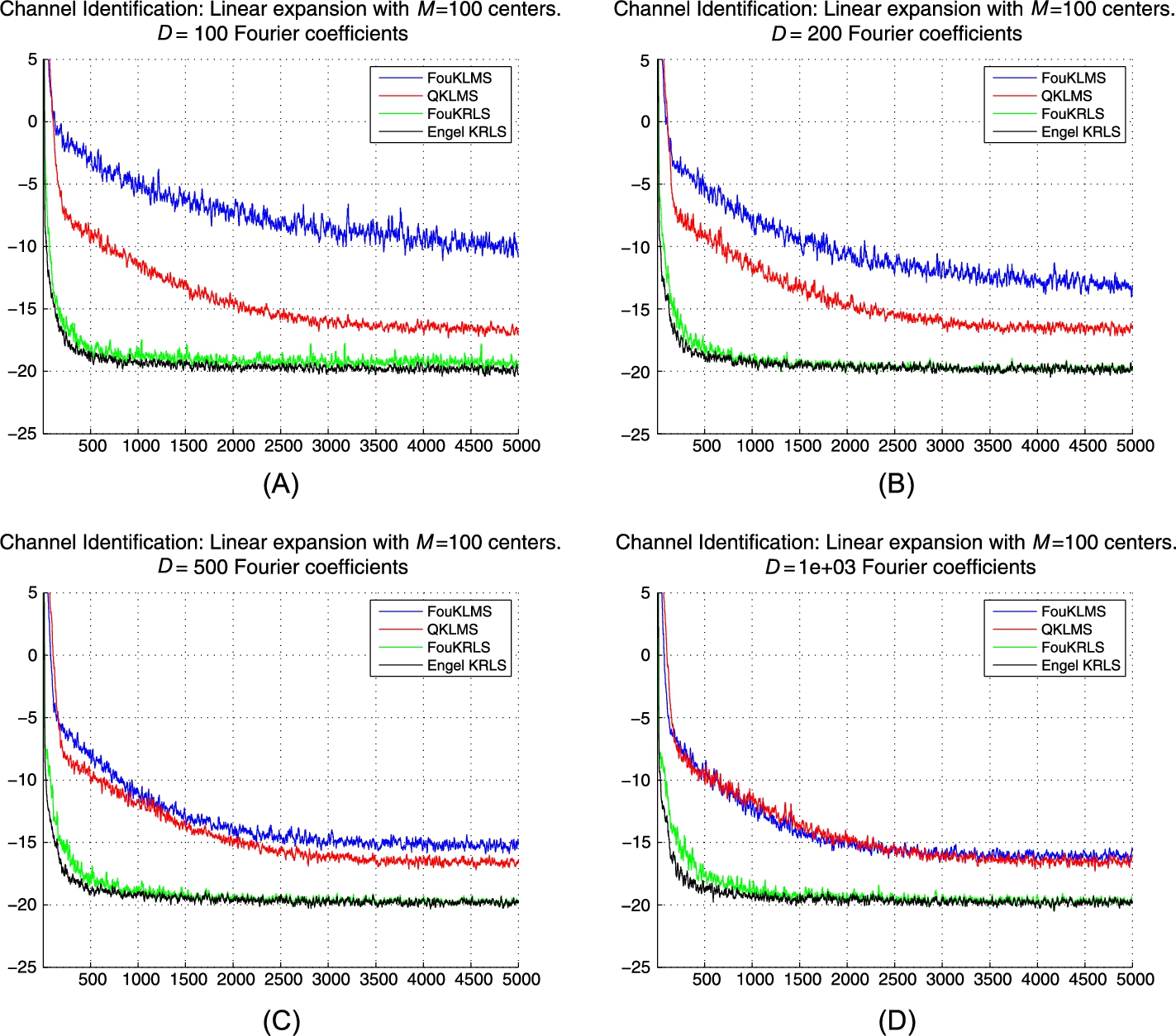
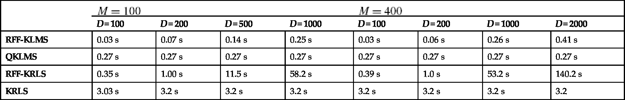
Table 7.2
Mean times needed for the KLMS and KRLS on a typical core i5 machine for M = 100 and M = 400
|
M=100
|
M=400
|
|||||||
|---|---|---|---|---|---|---|---|---|
| D = 100 | D = 200 | D = 500 | D = 1000 | D = 100 | D = 200 | D = 1000 | D = 2000 | |
| RFF-KLMS | 0.03 s | 0.07 s | 0.14 s | 0.25 s | 0.03 s | 0.06 s | 0.26 s | 0.41 s |
| QKLMS | 0.27 s | 0.27 s | 0.27 s | 0.27 s | 0.27 s | 0.27 s | 0.27 s | 0.27 s |
| RFF-KRLS | 0.35 s | 1.00 s | 11.5 s | 58.2 s | 0.39 s | 1.0 s | 53.2 s | 140.2 s |
| KRLS | 3.03 s | 3.2 s | 3.2 s | 3.2 s | 3.2 s | 3.2 s | 3.2 s | 3.2 |
7.3.5 Simulations—Classification
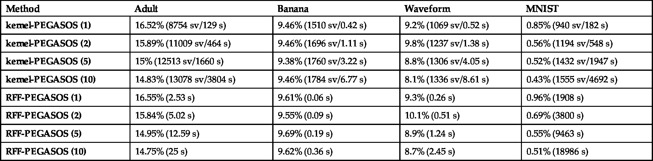
For the classification case, we have performed two sets of experiments. In the first set, we have compared the performances of the standard kernel-PEGASOS and the RFF-PEGASOS on four datasets downloaded from Leon Bottou's LASVM web page [18]. The chosen datasets are (a) the Adult dataset, (b) the Banana dataset (where we have used the first 4000 points as training data and the remaining 1300 as testing data), (c) the Waveform dataset (where we have used the first 4000 points as training data and the remaining 1000 as testing data) and (d) the MNIST dataset (for the task of classifying the digit 8 versus the rest). The sizes of the datasets are given in Table 7.4. Table 7.5 reports the test errors for each dataset and each method, along with the total number of support vectors after training (only for the kernel-PEGASOS) and the respective time in seconds (in parentheses). The experiments were performed on an i7-3770 machine using a MatLab implementation. The parameters used in each method are reported in Table 7.3. The parameters were selected after extensive trials to give the best possible accuracy. The parentheses (after the title of the method) indicate the number of times the algorithm passed through the entire dataset. As expected from the theoretical analysis of the corresponding complexities, for datasets with a large number of support vectors (such as Adult and Banana), RFF-PEGASOS requires significantly less time than its standard implementation. For datasets with a medium number of SVs (such as Waveform), this difference is diminishing, while for datasets with very few SVs (e.g., MNIST) kernel-PEGASOS can be significantly faster. We note that, for the MNIST database, RFF-PEGASOS attains a 0.47% test error percentage after 20 reruns (19000 s).
Table 7.3
Parameters for each classification method
| Method | Adult | Banana | Waveform | MNIST |
|---|---|---|---|---|
| Kernel-PEGASOS |
σ=√10λ=0.0000307
|
σ=0.7λ=1316
|
σ=√10λ=0.001
|
σ=4λ=10−7
|
| RFF-PEGASOS |
σ=√10λ=0.0000307D=2000

|
σ=0.7λ=1316D=200

|
σ=√10λ=0.001D=2000

|
σ=4λ=10−7D=100000

|
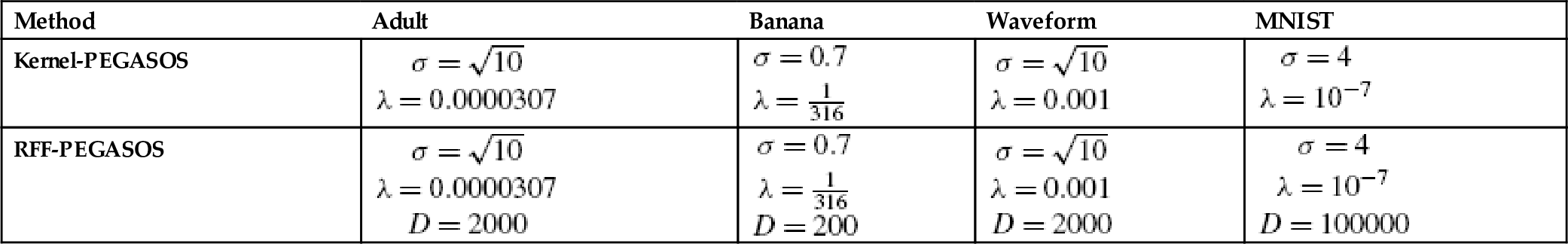
Table 7.4
Dataset Information
| Method | Adult | Banana | Waveform | MNIST |
|---|---|---|---|---|
| Training size | 32562 | 4000 | 4000 | 60000 |
| Testing size | 16282 | 1300 | 1000 | 10000 |
| dimensions | 123 | 2 | 21 | 784 |
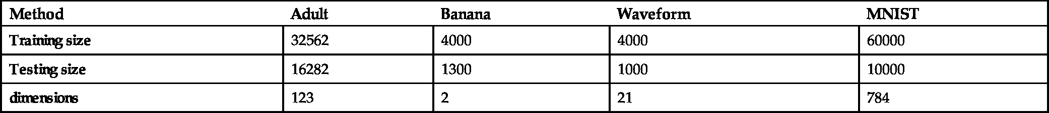
Table 7.5
Comparing the performances of kernel-PEGASOS and RFF-PEGASOS
| Method | Adult | Banana | Waveform | MNIST |
|---|---|---|---|---|
| kernel-PEGASOS (1) | 16.52% (8754 sv/129 s) | 9.46% (1510 sv/0.42 s) | 9.2% (1069 sv/0.52 s) | 0.85% (940 sv/182 s) |
| kernel-PEGASOS (2) | 15.89% (11009 sv/464 s) | 9.46% (1696 sv/1.11 s) | 9.8% (1237 sv/1.38 s) | 0.56% (1194 sv/548 s) |
| kernel-PEGASOS (5) | 15% (12513 sv/1660 s) | 9.38% (1760 sv/3.22 s) | 8.8% (1306 sv/4.05 s) | 0.52% (1432 sv/1947 s) |
| kernel-PEGASOS (10) | 14.83% (13078 sv/3804 s) | 9.46% (1784 sv/6.77 s) | 8.1% (1336 sv/8.61 s) | 0.43% (1555 sv/4692 s) |
| RFF-PEGASOS (1) | 16.55% (2.53 s) | 9.61% (0.06 s) | 9.3% (0.26 s) | 0.96% (1908 s) |
| RFF-PEGASOS (2) | 15.84% (5.02 s) | 9.55% (0.09 s) | 10.1% (0.51 s) | 0.69% (3800 s) |
| RFF-PEGASOS (5) | 14.95% (12.59 s) | 9.69% (0.19 s) | 8.9% (1.24 s) | 0.55% (9463 s) |
| RFF-PEGASOS (10) | 14.75% (25 s) | 9.62% (0.36 s) | 8.7% (2.45 s) | 0.51% (18986 s) |
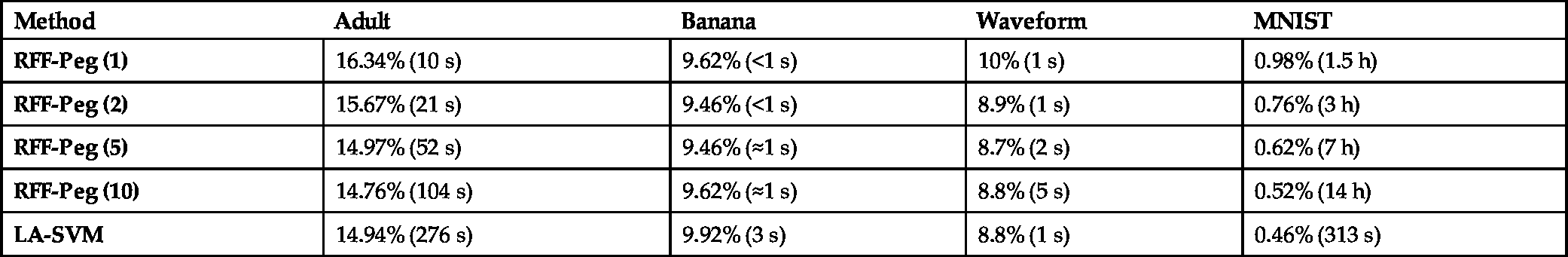
In the second set of experiments we tested the performance of RFF-PEGASOS and compared it with that of the LA-SVM [19]. LA-SVM is one of the most elegant and fast SVM training implementations. In order to compare running times we used a C implementation of the respective algorithms (as the C implementation of LA-SVM is publicly available on the web). The experiments were performed on an i5 650 machine running at 3.20 GHz with 6 Gb of RAM. The parameters for LA-SVM (shown in Table 7.3) have been taken from [19]. The results are shown in Table 7.6. Once more, we observe that for datasets with a large number of support vectors RFF-PEGASOS is faster. This is not the case however for datasets with a lower number of support vectors, where RFF-PEGASOS can be significantly slower.
Table 7.6
Comparing the performances of LA-SVM and RFF-PEGASOS
| Method | Adult | Banana | Waveform | MNIST |
|---|---|---|---|---|
| RFF-Peg (1) | 16.34% (10 s) | 9.62% (<1 s) | 10% (1 s) | 0.98% (1.5 h) |
| RFF-Peg (2) | 15.67% (21 s) | 9.46% (<1 s) | 8.9% (1 s) | 0.76% (3 h) |
| RFF-Peg (5) | 14.97% (52 s) | 9.46% (≈1 s) | 8.7% (2 s) | 0.62% (7 h) |
| RFF-Peg (10) | 14.76% (104 s) | 9.62% (≈1 s) | 8.8% (5 s) | 0.52% (14 h) |
| LA-SVM | 14.94% (276 s) | 9.92% (3 s) | 8.8% (1 s) | 0.46% (313 s) |
7.4 Online Distributed Learning With Kernels
Although the RFF methods, presented in Section 7.3, constitute a competitive alternative to existing online learning techniques in RKHS, the obtained results do not offer any significant real benefits from a practical point of view. In this section, we discuss the scenario of online distributed learning in RKHS, where it will be shown that the random Fourier features rationale can solve major open problems and lead to simple and elegant solutions.
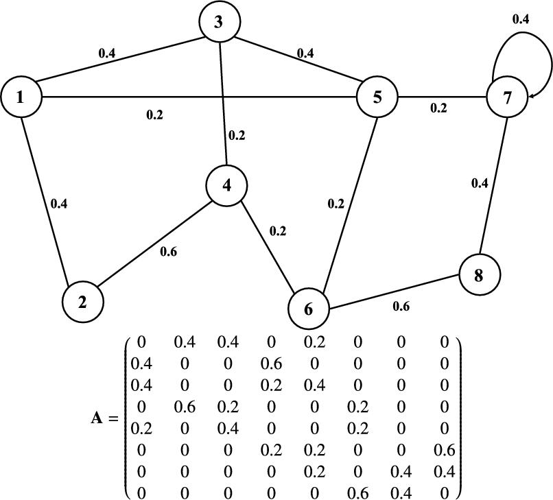
In the following, we consider K connected nodes, labeled k∈N={1,2,…K}![]() , which operate in cooperation to solve a specific learning task. This is a more general learning scenario compared to the one considered in Section 7.3, as the nodes are able to communicate with each other and exchange valuable information. The nodes comprising the network and the corresponding topology are represented as an undirected connected graph, consisting of K vertices (i.e., the nodes) and a set of edges that represent the communication between those nodes (see Fig. 7.3). The nodes that interact with node k are called the “neighbors” of k and the respective subset (that comprises the neighbors of k) is denoted as Nk⊆N
, which operate in cooperation to solve a specific learning task. This is a more general learning scenario compared to the one considered in Section 7.3, as the nodes are able to communicate with each other and exchange valuable information. The nodes comprising the network and the corresponding topology are represented as an undirected connected graph, consisting of K vertices (i.e., the nodes) and a set of edges that represent the communication between those nodes (see Fig. 7.3). The nodes that interact with node k are called the “neighbors” of k and the respective subset (that comprises the neighbors of k) is denoted as Nk⊆N![]() . Moreover, we assign a nonnegative weight ak,l
. Moreover, we assign a nonnegative weight ak,l![]() to the edge connecting node k to l, which is used by k to scale the data transmitted from l and vice versa (i.e., the confidence that node k assigns to node l). We collect all those weights into a K×K
to the edge connecting node k to l, which is used by k to scale the data transmitted from l and vice versa (i.e., the confidence that node k assigns to node l). We collect all those weights into a K×K![]() symmetric matrix A=(ak,l)
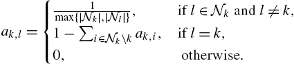
symmetric matrix A=(ak,l)![]() , such that the entries of the kth row of A contain the coefficients used by node k to scale the data arriving from its neighbors. Additionally, we assume that A is doubly stochastic, so that the weights of all incoming and outgoing “transmissions” sum to 1. Such a matrix can be generated using the Metropolis rule:
, such that the entries of the kth row of A contain the coefficients used by node k to scale the data arriving from its neighbors. Additionally, we assume that A is doubly stochastic, so that the weights of all incoming and outgoing “transmissions” sum to 1. Such a matrix can be generated using the Metropolis rule:
ak,l={1max{|Nk|,|Nl|},ifl∈Nkandl≠k,1−∑i∈Nk∖kak,i,ifl=k,0,otherwise.
Note that the topology considered here is similar to that of Chapter 9, which also deals with nonlinear learning over networks. Finally, we assume that each node, k, receives streaming data {(xk,n,yk(n)),n=1,2,…}![]() that are generated by yk(n)=g(xk,n)+ηk(n)
that are generated by yk(n)=g(xk,n)+ηk(n)![]() , where xk,n∈Rd
, where xk,n∈Rd![]() , yk(n)∈R
, yk(n)∈R![]() and ηk(n)
and ηk(n)![]() represents the respective noise, for the regression task. For classification, we assume that yk(n)=ϕ(f(xk,n))
represents the respective noise, for the regression task. For classification, we assume that yk(n)=ϕ(f(xk,n))![]() , where ϕ is a thresholding function, such that yk(n)∈{−1,1}
, where ϕ is a thresholding function, such that yk(n)∈{−1,1}![]() . In both tasks, the goal of each node is to obtain an estimate of the nonlinear function g, working in cooperation with its neighbors, so that a specific cost function is minimized.
. In both tasks, the goal of each node is to obtain an estimate of the nonlinear function g, working in cooperation with its neighbors, so that a specific cost function is minimized.
In the case where g is linear, i.e., it can be modeled as g(x)=θTx![]() , for some vector θ∈Rd
, for some vector θ∈Rd![]() , the problem has been studied extensively and several learning methods have been proposed based on the diffusion scheme (e.g., the diffusion LMS and the diffusion RLS). In a nutshell, these methods can be summarized in the following steps (this rationale is usually called Combine-Then-Adapt or CTA for short):
, the problem has been studied extensively and several learning methods have been proposed based on the diffusion scheme (e.g., the diffusion LMS and the diffusion RLS). In a nutshell, these methods can be summarized in the following steps (this rationale is usually called Combine-Then-Adapt or CTA for short):
- • Each node, k, receives the new data pair, i.e., (xk,n,yk(n))
 as well as the current estimates, θl,n−1
 , from all neighboring nodes, i.e., for all l∈Nk
 .
. - • Consequently, the node combines these estimates to a single one, ψk,n−1
 , taking into account the weights between the nodes, for example, ψk,n−1=∑l∈Nkak,lθl,n−1
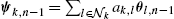 .
. - • Finally, the node exploits the combined estimate, ψk,n−1, as well as the newly received data to update the estimation. For example in diffusion LMS, where the mean square cost is minimized using a gradient descent rationale, the respective step update equation becomes θk,n=ψk,n−1+μek,nxk,n
 , where ek(n)=yk(n)−ψTk,n−1xk,n
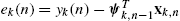 is the estimation error.
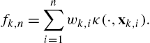
The implementation of such an approach in the context of RKHS presents significant challenges. The big difference lies in the fact that the estimation of the solution at each node is not a simple vector, but instead it is a function, which is expressed as a growing sum of kernel evaluations centered at the points observed by the specific node, i.e.,
fk,n=n∑i=1wk,iκ(⋅,xk,i).
Hence, the implementation of a straightforward CTA strategy would require from each node, k, to transmit its entire growing sum (i.e., the so-called dictionary, which comprises the coefficients wk,i![]() as well as the respective centers xk,i
as well as the respective centers xk,i![]() , for all i=1,2,…,n
, for all i=1,2,…,n![]() ) to all neighbors. This would significantly increase both the communication load among the nodes, as well as the computational cost at each node, since the size of the transmitted data would become increasingly larger as time evolves (as for every time instant, they gather the centers transmitted by all neighbors). Evidently, after a specific point in time this scheme would become so demanding that no machine would be able to carry on indefinitely. This is the rationale adopted in [20–22] for the case of KLMS. Alternatively, one could follow a pruning method similar to those applied for the standard KLMS and devise an efficient method to sparsify the solution at each node. However, this would require that, at each node, to somehow merge all the respective dictionaries (i.e., Eq. (7.11)) transmitted by its neighbors, at each time instant. For example, each node would have to search all the dictionaries that it receives from the neighboring nodes, for similar centers, and treat them as a single one. Alternatively, one could adopt a single prearranged dictionary (i.e., a specific set of centers) for all nodes and then fuse each observed point with the best-suited center. However, no such strategy has appeared in the respective literature, perhaps due to its increased complexity and lack of theoretical elegance.
) to all neighbors. This would significantly increase both the communication load among the nodes, as well as the computational cost at each node, since the size of the transmitted data would become increasingly larger as time evolves (as for every time instant, they gather the centers transmitted by all neighbors). Evidently, after a specific point in time this scheme would become so demanding that no machine would be able to carry on indefinitely. This is the rationale adopted in [20–22] for the case of KLMS. Alternatively, one could follow a pruning method similar to those applied for the standard KLMS and devise an efficient method to sparsify the solution at each node. However, this would require that, at each node, to somehow merge all the respective dictionaries (i.e., Eq. (7.11)) transmitted by its neighbors, at each time instant. For example, each node would have to search all the dictionaries that it receives from the neighboring nodes, for similar centers, and treat them as a single one. Alternatively, one could adopt a single prearranged dictionary (i.e., a specific set of centers) for all nodes and then fuse each observed point with the best-suited center. However, no such strategy has appeared in the respective literature, perhaps due to its increased complexity and lack of theoretical elegance.
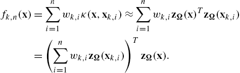
In the present chapter, we propose an alternative approach, which addresses the aforementioned problems. Once again, our starting point is the observation that the input–output relationship, y=f(x)![]() , can be closely approximated using the random Fourier features rationale (similar to Section 7.3). In particular, we see that
, can be closely approximated using the random Fourier features rationale (similar to Section 7.3). In particular, we see that
fk,n(x)=n∑i=1wk,iκ(x,xk,i)≈n∑i=1wk,izΩ(x)TzΩ(xk,i)=(n∑i=1wk,izΩ(xk,i))TzΩ(x).
Inspired by the last relation, we propose to approximate the desired input–output relationship as y=θTzΩ(x)![]() and follow a two-step procedure: (a) we map each observed point (xk,n,yk(n))
and follow a two-step procedure: (a) we map each observed point (xk,n,yk(n))![]() to (zΩ(xk,n),yk(n))
to (zΩ(xk,n),yk(n))![]() and then (b) we adopt a simple linear CTA diffusion strategy on the transformed points, where each node aims to estimate the vector θ∈RD
and then (b) we adopt a simple linear CTA diffusion strategy on the transformed points, where each node aims to estimate the vector θ∈RD![]() minimizing a specific (convex) cost function, L(x,y,θ)
minimizing a specific (convex) cost function, L(x,y,θ)![]() . We can summarize the proposed scheme for each node by the following relations:
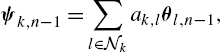
. We can summarize the proposed scheme for each node by the following relations:
ψk,n−1=∑l∈Nkak,lθl,n−1,
θk,n=ψk,n−1−μk,n∇θL(zΩ(xk,n),yk(n),ψk,n−1),
where μk,n![]() is the (possibly time varying) learning rate at the nth time instant on node k and ∇θL(zΩ(xk,n),yk,n,ψk,n−1)
is the (possibly time varying) learning rate at the nth time instant on node k and ∇θL(zΩ(xk,n),yk,n,ψk,n−1)![]() is the gradient, or any subgradient of L(x,y,θ)
is the gradient, or any subgradient of L(x,y,θ)![]() (with respect to θ), if the loss function is not differentiable. Eq. (7.12) refers to the fact that each node collects the past estimates from its neighbors to produce the combined estimate, ψk,n−1
(with respect to θ), if the loss function is not differentiable. Eq. (7.12) refers to the fact that each node collects the past estimates from its neighbors to produce the combined estimate, ψk,n−1![]() , while in Eq. (7.13) the most recent pair of observations is exploited to update the new estimate vector θk,n
, while in Eq. (7.13) the most recent pair of observations is exploited to update the new estimate vector θk,n![]() , employing a gradient descent–based rationale. We emphasize that L
, employing a gradient descent–based rationale. We emphasize that L![]() need not be differentiable. Hence, a large family of loss functions can be adopted. However, in this section, we focus on the following two types of cost functions:
need not be differentiable. Hence, a large family of loss functions can be adopted. However, in this section, we focus on the following two types of cost functions:
- • Mean squared error (for Regression): L(x,y,θ)=E[(y−θTx)2]
 .
. - • Hinge loss (for Classification): L(x,y,θ)=max(0,1−yθTx)
 .
.
We can write Eq. (7.12) and Eq. (7.13) more compactly using block-matrices as follows:
θ_n=A_θ_n−1−M_nG_n,
where θ_n:=(θT1,n,…,θTK,n)T∈RKD![]() is the collection of the estimations from each node, M_n:=diag{μ1,n,…,μK,n}⊗ID
is the collection of the estimations from each node, M_n:=diag{μ1,n,…,μK,n}⊗ID![]() is the collection of learning rates, A_:=A⊗ID
is the collection of learning rates, A_:=A⊗ID![]() and G_n:=[uT1,n,…,uTK,n]T
and G_n:=[uT1,n,…,uTK,n]T![]() , where uk,n=∇L(zΩ(xk,n),yk(n),ψk,n)
, where uk,n=∇L(zΩ(xk,n),yk(n),ψk,n)![]() comprises all (sub)gradients. Here, the symbol ⊗ denotes the matrix tensor product.
comprises all (sub)gradients. Here, the symbol ⊗ denotes the matrix tensor product.
The advantage of the proposed scheme is that each node transmits a single vector (i.e., its current estimate, θk,n![]() ) to its neighbors, instead of an entire dictionary of centers (and their respective coefficients) while the merging of the currently available estimates requires only a straightforward summation. However, we should point out that the new vector space, RD
) to its neighbors, instead of an entire dictionary of centers (and their respective coefficients) while the merging of the currently available estimates requires only a straightforward summation. However, we should point out that the new vector space, RD![]() , usually has a significantly larger dimension than the original input space Rd
, usually has a significantly larger dimension than the original input space Rd![]() . This may pose some communication obstacles; to this end, various suboptimal techniques can be used and have been proposed, e.g., [23].
. This may pose some communication obstacles; to this end, various suboptimal techniques can be used and have been proposed, e.g., [23].
7.4.1 Diffusion KLMS
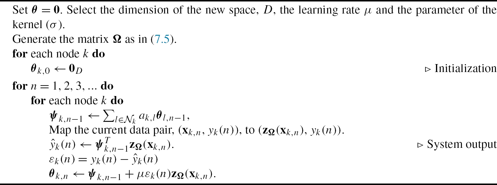
Adopting the mean square error in place of L![]() and estimating the gradient by its current measurement, the Random Fourier Features Diffusion KLMS (RFF-DKLMS) results, where Eq. (7.12) can be recast as
and estimating the gradient by its current measurement, the Random Fourier Features Diffusion KLMS (RFF-DKLMS) results, where Eq. (7.12) can be recast as
θk,n=ψk,n−1+μεk(n)zΩ(xk,n),
where εk(n)=yn−ψTk,n−1zΩ(xk,n)![]() . Algorithm 4 describes the proposed method in detail.
. Algorithm 4 describes the proposed method in detail.
Under certain general conditions, we can establish consensus (i.e., that all nodes converge to the same solution), [16], following the results of the standard Diffusion LMS (e.g., [24,25]). To this end, we will assume that the data pairs are generated by
yk(n)=M∑m=1αmκ(cm,xk,n)+ηk(n),
where c1,…,cM![]() are fixed centers, xk,n
are fixed centers, xk,n![]() are zero-mean i.i.d, samples drawn from the Gaussian distribution with covariance matrix σ2XId
are zero-mean i.i.d, samples drawn from the Gaussian distribution with covariance matrix σ2XId![]() and ηk(n)
and ηk(n)![]() are independent and identically distributed noise samples drawn from N(0,σ2η)
are independent and identically distributed noise samples drawn from N(0,σ2η)![]() . Hence, we have
. Hence, we have
yk(n)=M∑m=1αmEω,b[zω,b(cm)zω,b(xk,n)]+ηk(n)≈αTZTΩzΩ(xk,n)+ϵk(n)+ηk(n)=θTozΩ(xk,n)+ϵk(n)+ηk(n),
where ZΩ=(zΩ(c1),…,zΩ(cM))![]() , α=(α1,…,αM)T
, α=(α1,…,αM)T![]() , θo=ZΩα
, θo=ZΩα![]() and ϵk(n)
and ϵk(n)![]() is the approximation error between the noise-free component of yk(n)
is the approximation error between the noise-free component of yk(n)![]() (evaluated only by the linear kernel expansion of Eq. (7.16)) and the approximation of this component using random Fourier features, i.e., ϵk(n)=∑Mm=1αmκ(cm,xk,n)−θTozΩ(xk,n)
(evaluated only by the linear kernel expansion of Eq. (7.16)) and the approximation of this component using random Fourier features, i.e., ϵk(n)=∑Mm=1αmκ(cm,xk,n)−θTozΩ(xk,n)![]() . Using block-matrices we can derive the following, more compact, formulation for the entire network:
. Using block-matrices we can derive the following, more compact, formulation for the entire network:
y_n=V_Tnθ_o+ϵ_n+η_n,
where
- • y_n:=(y1(n),y2(n),…,yK(n))T
 ,
, - • V_n:=diag(zΩ(x1,n),zΩ(x2,n),…,zΩ(xK,n))
 , is a DK×K
 matrix,
 - • θ_o=(θTo,θTo,…,θTo)T∈RDK
 ,
, - • ϵ_n=(ϵ1(n),ϵ2(n),…,ϵK(n))T∈RK
 ,
, - • η_n=(η1(n),η2(n),…,ηK(n))T∈RK
 .
.
Let x1,…,xK∈Rd![]() , y_∈RK
, y_∈RK![]() , be the random variables that generate the measurements of the nodes and
, be the random variables that generate the measurements of the nodes and
V_=diag(zΩ(x1),zΩ(x2),…,zΩ(xK))
be the DK×K![]() matrix that collects the transformed random variables for the whole network. Moreover, let R_=E[V_V_T]
matrix that collects the transformed random variables for the whole network. Moreover, let R_=E[V_V_T]![]() be the DK×DK
be the DK×DK![]() respective autocorrelation matrix. It is not difficult to see that R_
respective autocorrelation matrix. It is not difficult to see that R_![]() can be given in a block form as R_=E[V_V_T]=diag(Rzz,Rzz…,Rzz)
can be given in a block form as R_=E[V_V_T]=diag(Rzz,Rzz…,Rzz)![]() , where Rzz=E[zΩ(xk)zΩ(xk)T]
, where Rzz=E[zΩ(xk)zΩ(xk)T]![]() , for all k=1,2,…,K
, for all k=1,2,…,K![]() . We can prove that, under certain general conditions, the autocorrelation matrix R is invertible (see [16] for the proof).
. We can prove that, under certain general conditions, the autocorrelation matrix R is invertible (see [16] for the proof).
Lemma 1
Consider a selection of samples ω1,ω2,…,ωD![]() , drawn from (7.6) such that ωi≠ωj
, drawn from (7.6) such that ωi≠ωj![]() , for any i≠j
, for any i≠j![]() . Then both Rzz
. Then both Rzz![]() and R_=E[V_V_T]
and R_=E[V_V_T]![]() are strictly positive definite (hence invertible) matrices.
are strictly positive definite (hence invertible) matrices.
Moreover, as Rzz![]() is positive definite (this has been also discussed in Section 7.4.1), the respective eigenvalues satisfy 0<λ1⩽λ2⩽⋯⩽λD
is positive definite (this has been also discussed in Section 7.4.1), the respective eigenvalues satisfy 0<λ1⩽λ2⩽⋯⩽λD![]() . In this case, the optimal solution is given by
. In this case, the optimal solution is given by
θ_⁎=argminθ_E[‖y_−V_Tθ_‖2]=E[V_V_T]−1E[V_y_]=E[V_V_T]−1(E[V_(V_Tθ_o+ϵ_+η_)])=E[V_V_T]−1(E[V_V_T]θ_o+E[V_ϵ_]+E[V_η_])=E[V_V_T]−1(E[V_V_T]θ_o+E[V_ϵ_]),
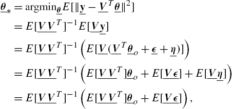
where for the last relation we have used the notion that η is a zero mean vector representing noise and that V_![]() and η_
and η_![]() are independent. For large enough D, the approximation error vector ϵ_
are independent. For large enough D, the approximation error vector ϵ_![]() approaches 0K
approaches 0K![]() , hence the optimal solution becomes
, hence the optimal solution becomes
θ_⁎=θ_o+E[V_V_T]−1E[V_ϵ_]≈θ_o.
Since we work under the assumption that ϵ_![]() approaches 0K
approaches 0K![]() , we can say that Eq. (7.17) can be closely approximated by y_n≈V_nθ_o+η_n
, we can say that Eq. (7.17) can be closely approximated by y_n≈V_nθ_o+η_n![]() . This actually means that the RFF-DKLMS is nothing more than the standard diffusion LMS applied to the data pairs {(zΩ(xk,n),yk(n),k=1,…,K,n=1,2…}
. This actually means that the RFF-DKLMS is nothing more than the standard diffusion LMS applied to the data pairs {(zΩ(xk,n),yk(n),k=1,…,K,n=1,2…}![]() . However, the difference is that the input vectors zΩ(xk,n)
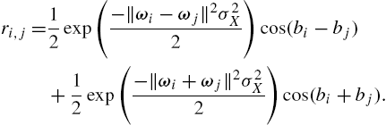
. However, the difference is that the input vectors zΩ(xk,n)![]() may have nonzero mean and do not follow, necessarily, the Gaussian distribution. In fact we can prove that, if xk,n∼N(0,σXId)
may have nonzero mean and do not follow, necessarily, the Gaussian distribution. In fact we can prove that, if xk,n∼N(0,σXId)![]() , then the entries of Rzz
, then the entries of Rzz![]() can be evaluated as
can be evaluated as
ri,j=12exp(−‖ωi−ωj‖2σ2X2)cos(bi−bj)+12exp(−‖ωi+ωj‖2σ2X2)cos(bi+bj).
Consequently, the available results regarding convergence and stability of diffusion LMS (e.g., [24,26]) cannot be applied here directly, as in these works the inputs are assumed to be zero mean Gaussian (to simplify the formulas related to stability). However, it is possible to end up with similar conclusions (the proofs are given in [16]).
Proposition 1
Proposition 2
For stability in the mean square sense, we must ensure that both μ and A satisfy
ρ(ID2K2−μ(R_⊠IDK+IDK⊠R_)(A_⊠A_))<1,
where ⊠ denotes the unbalanced block Kronecker product (see [27]) and ρ(⋅)![]() denotes the spectral radius of the respective matrix.
denotes the spectral radius of the respective matrix.
7.4.2 Diffusion PEGASOS
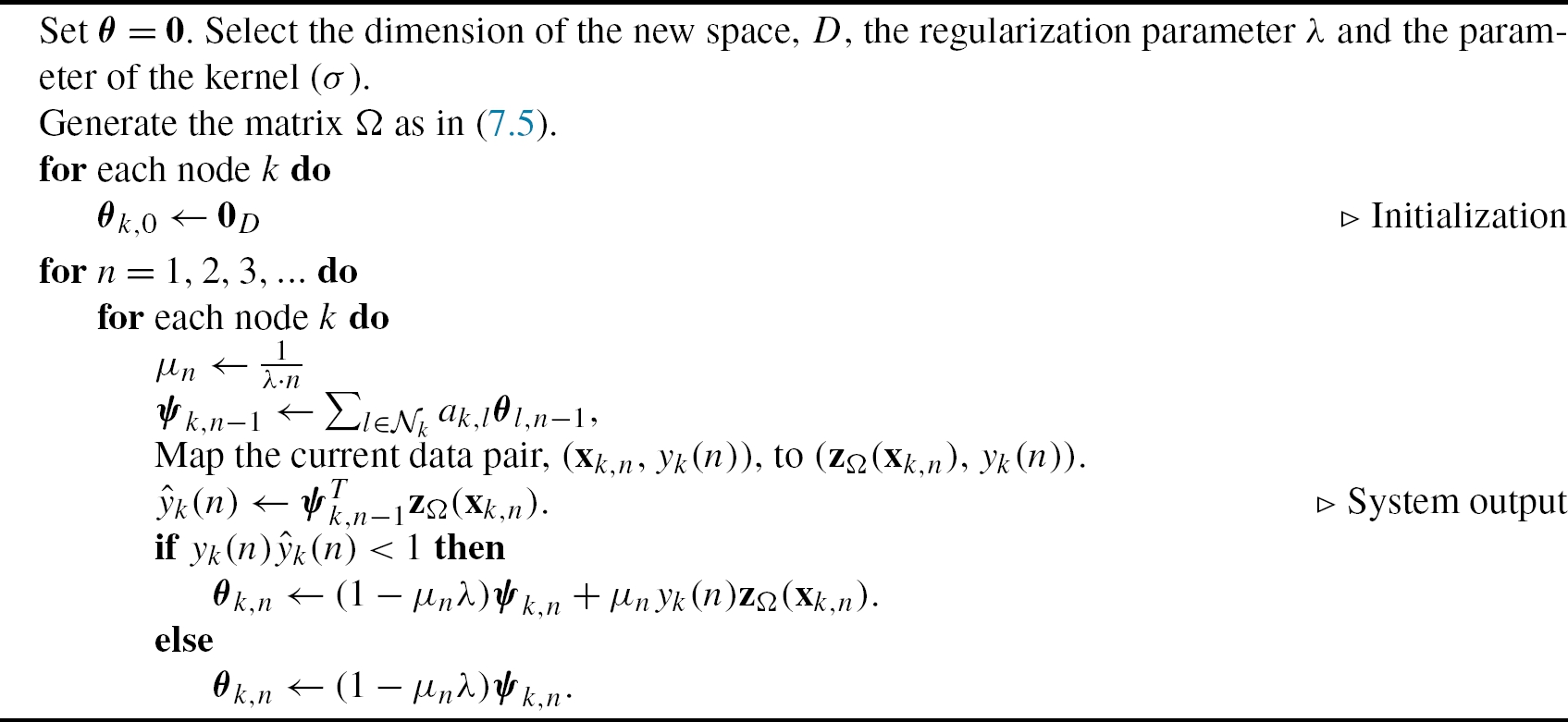
For the case of classification tasks, we can adopt the regularized hinge loss function, for a specific value of the regularization parameter, λ, and get a diffusion version of PEGASOS, in its full online version (see Algorithm 5). In this case, the gradient becomes
∇θL(x,y,θ)=λθ−I+(1−yθTzΩ(x))yzΩ(x),
where I+![]() is the indicator function of (0,+∞)
is the indicator function of (0,+∞)![]() , which takes a value of 1, if its argument belongs in (0,+∞)
, which takes a value of 1, if its argument belongs in (0,+∞)![]() , and zero otherwise. Hence the step update equation of the algorithm becomes
, and zero otherwise. Hence the step update equation of the algorithm becomes
θk,n=(1−1n)ψk,n−1+I+(1−ynψTk,n−1zΩ(xk,n))yk(n)λnzΩ(xk,n),
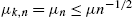
where, following [17], we have used a decreasing learning rate, μn=1λn![]() . Recall, however, that we can write the update scheme more compactly by Eq. (7.14), setting Mn=diag(1/(λn),…,1/(λn))⊗ID
. Recall, however, that we can write the update scheme more compactly by Eq. (7.14), setting Mn=diag(1/(λn),…,1/(λn))⊗ID![]() .
.
We can prove that all nodes converge to the same solution using the result from [16], where it is proven that the general update scheme described by Eq. (7.14) achieves asymptotic consensus, if the following assumptions are satisfied:
- Assumption 1: The step size is time decaying and is bounded by the inverse square root of time, i.e., μk,n=μn⩽μn−1/2
 .
. - Assumption 2: The norm of the transformed input is bounded, i.e., there is U1>0
 , such that ‖zΩ(xk,n)‖⩽U1,∀k∈N,∀n∈N
 . Furthermore, yk,n
 is bounded, i.e., there is V>0
 , such that |yk,n|⩽V,∀k∈N,∀n∈N
 .
. - Assumption 3: The estimates are bounded, i.e., there is U2>0
 , such that ‖θk,n‖⩽U2,∀k∈N
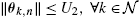 , ∀n∈N
 .
. - Assumption 4: The matrix comprising the combination weights, i.e., A, is doubly stochastic.
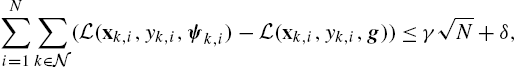
Moreover, in [16], it is shown that the regret is sublinearly bounded, which means that on average the algorithm performs at least as well as the best fixed strategy.
Proposition 3
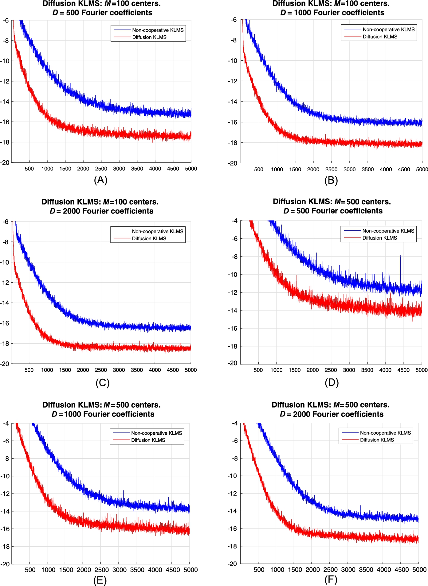
7.4.3 Simulations—Diffusion KLMS
In order to demonstrate that the estimation provided by the cooperative strategy is better than having each node working alone, we follow a similar experimental setup as in Section 7.3.4. Each realization of the experiments uses a different random connected graph with K=10![]() nodes and with a probability of attachment per node equal to 0.25 (i.e., there is a 25% probability that a specific node k is connected to any other node l). The graphs are generated using MIT's random_graph routine (see [28]) and their adjacency matrices, A, using the Metropolis rule (resulting in graphs with mean algebraic connectivity around 0.69). For the noncooperative case, we simply used a graph that connects each node to itself, i.e., A=I10
nodes and with a probability of attachment per node equal to 0.25 (i.e., there is a 25% probability that a specific node k is connected to any other node l). The graphs are generated using MIT's random_graph routine (see [28]) and their adjacency matrices, A, using the Metropolis rule (resulting in graphs with mean algebraic connectivity around 0.69). For the noncooperative case, we simply used a graph that connects each node to itself, i.e., A=I10![]() . All parameters were optimized (after trials) to give the lowest MSE. The algorithms were implemented in Matlab and the experiments were performed on an i7-3770 machine running at 3.4 GHz with 32 Mb of RAM. Similar to Section 7.3.4, we generated 5000 data pairs for each node using the following model:
. All parameters were optimized (after trials) to give the lowest MSE. The algorithms were implemented in Matlab and the experiments were performed on an i7-3770 machine running at 3.4 GHz with 32 Mb of RAM. Similar to Section 7.3.4, we generated 5000 data pairs for each node using the following model:
yk(n)=M∑m=1amκ(cm,xk,n)+ηk(n),
where xk,n∈R5![]() are drawn from N(0,I5)
are drawn from N(0,I5)![]() and the noise are independent and identically distributed Gaussian samples with ση=0.1
and the noise are independent and identically distributed Gaussian samples with ση=0.1![]() . The parameters of the expansion (i.e., a1,…,aM
. The parameters of the expansion (i.e., a1,…,aM![]() ) are drawn from N(0,25)
) are drawn from N(0,25)![]() , the kernel parameter σ is set to 5 and the learning rate is set to μ=1
, the kernel parameter σ is set to 5 and the learning rate is set to μ=1![]() . Fig. 7.4 shows the evolution of the MSE over all network nodes for 100 realizations of the experiment (for various values of D and M). We note that the selected value of the step size satisfies the conditions of Proposition 1.
. Fig. 7.4 shows the evolution of the MSE over all network nodes for 100 realizations of the experiment (for various values of D and M). We note that the selected value of the step size satisfies the conditions of Proposition 1.
7.4.4 Simulations—Diffusion PEGASOS
We have tested the performance of Diffusion-PEGASOS versus the noncooperative kernel Pegasus on the same four datasets that were used in Section 7.3.5. In all experiments, we generated random graphs (using MIT's random_graph routine) and compared the proposed diffusion method versus the respective noncooperative strategy (where each node works independent of the rest). Similar to Section 7.4.3, a different random connected graph with K=5![]() or K=20
or K=20![]() nodes was generated, for each realization of the experiments. The probability of attachment per node was set equal to 0.2 and the respective adjacency matrix, A, of each graph was generated using the Metropolis rule. For the noncooperative strategies, we used a graph that connects each node to itself, i.e., A=I5
nodes was generated, for each realization of the experiments. The probability of attachment per node was set equal to 0.2 and the respective adjacency matrix, A, of each graph was generated using the Metropolis rule. For the noncooperative strategies, we used a graph that connects each node to itself, i.e., A=I5![]() or A=I20
or A=I20![]() , respectively. Moreover, for each realization, the corresponding dataset was randomly split into K subsets of equal size (one for every node). All parameters were optimized (after trials) to give the lowest number of test errors. Their values are reported in Table 7.9. The algorithms were implemented in Matlab and the experiments were performed on an i7-3770 machine running at 3.4 GHz with 32 Gb of RAM. Tables 7.7 and 7.8 report the mean test errors obtained by both procedures. The number inside the parentheses indicates the times of data reuse (i.e., running the algorithm again over the same data, albeit with a continuously decreasing step size μn
, respectively. Moreover, for each realization, the corresponding dataset was randomly split into K subsets of equal size (one for every node). All parameters were optimized (after trials) to give the lowest number of test errors. Their values are reported in Table 7.9. The algorithms were implemented in Matlab and the experiments were performed on an i7-3770 machine running at 3.4 GHz with 32 Gb of RAM. Tables 7.7 and 7.8 report the mean test errors obtained by both procedures. The number inside the parentheses indicates the times of data reuse (i.e., running the algorithm again over the same data, albeit with a continuously decreasing step size μn![]() ), which has been suggested to improve the classification accuracy of PEGASOS (see [17]). For example, the number 2 indicates that the algorithm runs over a dataset of double size, that contains the same data pairs twice. For the three first datasets (Adult, Banana, Waveform) we have run 100 realizations of the experiment, while for the fourth (MNIST) we have run only 10 (to save time). Besides the ADULT dataset, all other simulations show that the distributed implementation significantly outperforms the noncooperative one. For that particular dataset, we observe that for a single run the noncooperative strategy behaves better (for K=20
), which has been suggested to improve the classification accuracy of PEGASOS (see [17]). For example, the number 2 indicates that the algorithm runs over a dataset of double size, that contains the same data pairs twice. For the three first datasets (Adult, Banana, Waveform) we have run 100 realizations of the experiment, while for the fourth (MNIST) we have run only 10 (to save time). Besides the ADULT dataset, all other simulations show that the distributed implementation significantly outperforms the noncooperative one. For that particular dataset, we observe that for a single run the noncooperative strategy behaves better (for K=20![]() ), but as data reuse increases the distributed implementation reaches lower error floors.
), but as data reuse increases the distributed implementation reaches lower error floors.
Table 7.7
Comparing the performances of the Diffusion PEGASOS versus the noncooperative PEGASOS for graphs with K = 5 nodes
| Method | Adult | Banana | Waveform | MNIST |
|---|---|---|---|---|
| Diffusion-PEGASOS (1) | 19% | 11.80% | 11.82% | 0.79% |
| Diffusion-PEGASOS (2) | 17.43% | 10.84% | 10.49% | 0.68% |
| Diffusion-PEGASOS (5) | 15.87% | 10.34% | 9.56% | 0.59% |
| Noncooperative-PEGASOS (1) | 19.11% | 14.52% | 13.75% | 1.42% |
| Noncooperative-PEGASOS (2) | 18.31% | 12.52% | 12.59% | 1.19% |
| Noncooperative-PEGASOS (5) | 17.29% | 11.32% | 11.86% | 1.01% |
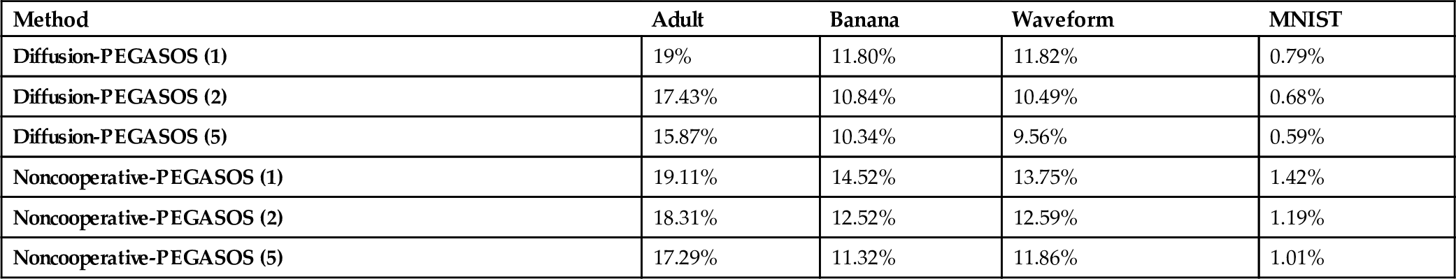
Table 7.8
Comparing the performances of the Distributed PEGASOS versus the noncooperative PEGASOS for graphs with K = 20 nodes
| Method | Adult | Banana | Waveform | MNIST |
|---|---|---|---|---|
| Diffusion-PEGASOS (1) | 24.04% | 16.38% | 16.26% | 1.03% |
| Diffusion-PEGASOS (2) | 22.34% | 13.23% | 13.93% | 0.77% |
| Diffusion-PEGASOS (5) | 18.94% | 10.83% | 11.20% | 0.57% |
| Noncooperative-PEGASOS (1) | 20.81% | 21.74% | 18.40% | 2.93% |
| Noncooperative-PEGASOS (2) | 20.52% | 18.64% | 16.54% | 2.19% |
| Noncooperative-PEGASOS (5) | 19.88% | 15.96% | 14.86% | 1.87% |
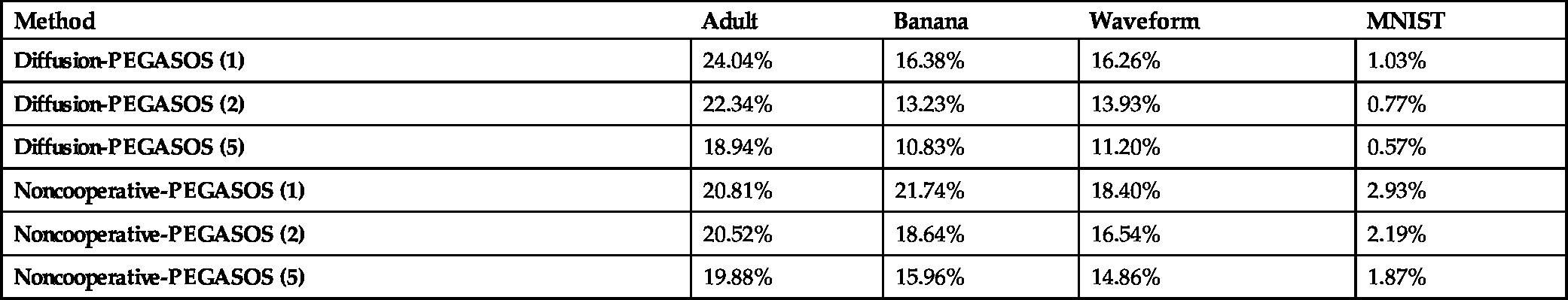
Table 7.9
Parameters for each method
| Method | Adult | Banana | Waveform | MNIST |
|---|---|---|---|---|
| Kernel-PEGASOS |
σ=√10λ=0.0000307
|
σ=0.7λ=1316
|
σ=√10λ=0.001
|
σ=4λ=10−7
|
| RFF-PEGASOS |
σ=√10λ=0.0000307D=2000
|
σ=0.7λ=1316D=200
|
σ=√10λ=0.001D=2000
|
σ=4λ=10−7D=100000
|

7.5 Conclusions
In this chapter, we presented an alternative path for designing online kernel-based learning methods. Instead of relying on the typical growing sum, the presented approach suggests to approximate the solution using randomly sampled Fourier features of the kernel. This is equivalent to transforming the training data to a Euclidean space of larger dimension, thus leading to linear fixed-budget strategies. Moreover, the proposed approach can be exploited to derive online distributed schemes for learning over networks, where the nodes cooperate to find a combined solution, based on the combine-then-adapt rationale. We stress out that this is the first practical scheme for kernel-based distributed learning that has been proposed in the literature so far. The provided simulations verify the validity of the proposed approach.