
Kernel-Based Inference of Functions Over Graphs
Vassilis N. Ioannidis⁎; Meng Ma⁎; Athanasios N. Nikolakopoulos⁎; Georgios B. Giannakis⁎; Daniel Romero† ⁎University of Minnesota, Minneapolis, MN, United States
†University of Agder, Grimstad, Norway
Abstract
The study of networks has witnessed an explosive growth over the past decades with several ground-breaking methods introduced. A particularly interesting—and prevalent in several fields of study—problem is that of inferring a function defined over the nodes of a network. This work presents a versatile kernel-based framework for tackling this inference problem that naturally subsumes and generalizes the reconstruction approaches put forth recently for the signal processing by the community studying graphs. Both the static and the dynamic settings are considered along with effective modeling approaches for addressing real-world problems. The analytical discussion herein is complemented with a set of numerical examples, which showcase the effectiveness of the presented techniques, as well as their merits related to state-of-the-art methods.
Keywords
Signal processing on graphs; Kernel-based learning; Graph function reconstruction; Dynamic graphs; Kernel Kalman filter
Acknowledgements
The research was supported by NSF grants 1442686, 1500713, 1508993, 1509040, and 1739397.
8.1 Introduction
Numerous applications arising in diverse disciplines involve inference over networks [1]. Modeling nodal attributes as signals that take values over the vertices of the underlying graph allows the associated inference tasks to leverage node dependencies captured by the graph structure. In many real settings one often affords to work with only a limited number of node observations due to inherent restrictions particularly to the inference task at hand. In social networks, for example, individuals may be reluctant to share personal information; in sensor networks the nodes may report observations sporadically in order to save energy; in brain networks acquiring node samples may involve invasive procedures (e.g., electrocorticography). In this context, a frequently encountered challenge that often emerges is that of inferring the attributes for every node in the network given the attributes for a subset of nodes. This is typically formulated as the task of reconstructing a function defined on the nodes [1–6], given information about some of its values.
Reconstruction of functions over graphs has been studied by the machine learning community, in the context of semisupervised learning under the term of transductive regression and classification [6–8]. Existing approaches assume “smoothness” with respect to the graph—in the sense that neighboring vertices have similar values—and devise nonparametric methods [2,3,6,9] targeting primarily the task of reconstructing binary-valued signals. Function estimation has also been investigated recently by the community of signal processing on graphs (SPoG) under the term signal reconstruction [10–17]. Most of such approaches commonly adopt parametric estimation tools and rely on bandlimitedness, by which the signal of interest is assumed to lie in the span of the B principal eigenvectors of the graph's Laplacian (or adjacency) matrix.
This chapter cross-pollinates ideas arising from both communities and presents a unifying framework for tackling signal reconstruction problems both in the traditional time-invariant, as well as in the more challenging time varying setting. We begin by a comprehensive presentation of kernel-based learning for solving problems of signal reconstruction over graphs (Section 8.2). Data-driven techniques are then presented based on multikernel learning (MKL) that enables combining optimally the kernels in a given dictionary and simultaneously estimating the graph function by solving a single optimization problem (Section 8.2.3). For the case where prior information is available, semiparametric estimators are discussed that can incorporate seamlessly structured prior information into the signal estimators (Section 8.2.4). We then move to the problem of reconstructing time evolving functions on dynamic graphs (Section 8.3). The kernel-based framework is now extended to accommodate the time evolving setting building on the notion of graph extension, specific choices of which can lend themselves to a reduced complexity online solver (Section 8.3.1). Next, a more flexible model is introduced that captures multiple forms of time dynamics, and kernel-based learning is employed to derive an online solver that effects online MKL by selecting the optimal combination of kernels on-the-fly (Section 8.3.2). Our analytical exposition, in both parts, is supplemented with a set of numerical tests based on both real and synthetic data that highlight the effectiveness of the methods, while providing examples of interesting realistic problems that they can address.
Notation: Scalars are denoted by lowercase characters, vectors by bold lowercase, matrices by bold uppercase; (A)m,n![]() is the (m,n)
is the (m,n)![]() th entry of matrix A; superscripts T and † respectively denote transpose and pseudoinverse. If A:=[a1,…,aN]
th entry of matrix A; superscripts T and † respectively denote transpose and pseudoinverse. If A:=[a1,…,aN]![]() , then vec{A}:=[aT1,…,aTN]T:=a
, then vec{A}:=[aT1,…,aTN]T:=a![]() . With N×N
. With N×N![]() matrices {At}Tt=1
matrices {At}Tt=1![]() and {Bt}Tt=2
and {Bt}Tt=2![]() satisfying At=ATt∀t
satisfying At=ATt∀t![]() , btridiag{A1,…,AT;B2,…,BT}
, btridiag{A1,…,AT;B2,…,BT}![]() represents the symmetric block tridiagonal matrix. Symbols ⊙, ⊗ and ⊕, respectively, denote the element-wise (Hadamard) matrix product, Kronecker product and Kronecker sum, the latter being defined for A∈RM×M
represents the symmetric block tridiagonal matrix. Symbols ⊙, ⊗ and ⊕, respectively, denote the element-wise (Hadamard) matrix product, Kronecker product and Kronecker sum, the latter being defined for A∈RM×M![]() and B∈RN×N
and B∈RN×N![]() as A⊕B:=A⊗IN+IM⊗B
as A⊕B:=A⊗IN+IM⊗B![]() . The nth column of the identity matrix IN
. The nth column of the identity matrix IN![]() is represented by iN,n
is represented by iN,n![]() . If A∈RN×N
. If A∈RN×N![]() is positive definite and x∈RN
is positive definite and x∈RN![]() , then ‖x‖2A:=xTA−1x
, then ‖x‖2A:=xTA−1x![]() and ‖x‖2:=‖x‖IN
and ‖x‖2:=‖x‖IN![]() . The cone of N×N
. The cone of N×N![]() positive definite matrices is denoted by SN+
positive definite matrices is denoted by SN+![]() . Finally, δ[⋅]
. Finally, δ[⋅]![]() stands for the Kronecker delta and E
stands for the Kronecker delta and E![]() for expectation.
for expectation.
8.2 Reconstruction of Functions Over Graphs
Before giving the formal problem statement, it is instructive to start with the basic definitions that will be used throughout this chapter.
Definitions: A graph can be specified by a tuple G:=(V,A)![]() , where V:={v1,…,vN}
, where V:={v1,…,vN}![]() is the vertex set and A is the N×N
is the vertex set and A is the N×N![]() adjacency matrix, whose (n,n′)
adjacency matrix, whose (n,n′)![]() th entry, An,n′≥0
th entry, An,n′≥0![]() , denotes the nonnegative edge weight between vertices vn
, denotes the nonnegative edge weight between vertices vn![]() and vn′
and vn′![]() . For simplicity, it is assumed that the graph has no self-loops, i.e., An,n=0,∀vn∈V
. For simplicity, it is assumed that the graph has no self-loops, i.e., An,n=0,∀vn∈V![]() . This chapter focuses on undirected graphs, for which An′,n=An,n′∀vn,vn′∈V
. This chapter focuses on undirected graphs, for which An′,n=An,n′∀vn,vn′∈V![]() . A graph is said to be unweighted if An,n′
. A graph is said to be unweighted if An,n′![]() is either 0 or 1. The edge set is defined as E:={(vn,vn′)∈V×V:An,n′≠0}
is either 0 or 1. The edge set is defined as E:={(vn,vn′)∈V×V:An,n′≠0}![]() . Two vertices vn
. Two vertices vn![]() and vn′
and vn′![]() are adjacent, connected or neighbors if (vn,vn′)∈E
are adjacent, connected or neighbors if (vn,vn′)∈E![]() . The Laplacian matrix is defined as L:=diag{A1}−A
. The Laplacian matrix is defined as L:=diag{A1}−A![]() and is symmetric and positive semidefinite [1, Chapter 2]. A real-valued function (or signal) on a graph is a map f:V→R
and is symmetric and positive semidefinite [1, Chapter 2]. A real-valued function (or signal) on a graph is a map f:V→R![]() . The value f(v)
. The value f(v)![]() represents an attribute or feature of v∈V
represents an attribute or feature of v∈V![]() , such as age, political alignment or annual income of a person in a social network. Signal f is thus represented by f:=[f(v1),…,f(vN)]T
, such as age, political alignment or annual income of a person in a social network. Signal f is thus represented by f:=[f(v1),…,f(vN)]T![]() .
.
Problem statement. Suppose that a collection of noisy samples (or observations) {ys|ys=f(vns)+es}Ss=1![]() is available, where es
is available, where es![]() models noise and S:={n1,…,nS}
models noise and S:={n1,…,nS}![]() contains the indices 1⩽n1<⋯<nS⩽N
contains the indices 1⩽n1<⋯<nS⩽N![]() of the sampled vertices, with S≤N
of the sampled vertices, with S≤N![]() . Given {(ns,ys)}Ss=1
. Given {(ns,ys)}Ss=1![]() and assuming knowledge of G
and assuming knowledge of G![]() , the goal is to estimate f. This will provide estimates of f(v)
, the goal is to estimate f. This will provide estimates of f(v)![]() both at observed and unobserved vertices. By defining y:=[y1,…,yS]T
both at observed and unobserved vertices. By defining y:=[y1,…,yS]T![]() , the observation model is summarized as
, the observation model is summarized as
y=Sf+e,
where e:=[e1,…,eS]T![]() and S is a known S×N
and S is a known S×N![]() binary sampling matrix with entries (s,ns)
binary sampling matrix with entries (s,ns)![]() , s=1,…,S
, s=1,…,S![]() , set to one and the rest set to zero.
, set to one and the rest set to zero.
8.2.1 Kernel Regression
Kernel methods constitute the “workhorse” of machine learning for nonlinear function estimation [18]. Their popularity can be attributed to their simplicity, flexibility and good performance. Here, we present kernel regression as a unifying framework for graph signal reconstruction along with the so-called representer theorem.
Kernel regression seeks an estimate of f in a reproducing kernel Hilbert space (RKHS) H![]() , which is the space of functions f:V→R
, which is the space of functions f:V→R![]() defined as
defined as
H:={f:f(v)=N∑n=1αnκ(v,vn),αn∈R},
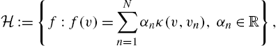
where the kernel map κ:V×V→R![]() is any function defining a symmetric and positive semidefinite N×N
is any function defining a symmetric and positive semidefinite N×N![]() matrix with entries [K]n,n′:=κ(vn,vn′)
matrix with entries [K]n,n′:=κ(vn,vn′)![]() [19]. Intuitively, κ(v,v′)
[19]. Intuitively, κ(v,v′)![]() is a basis function in (8.2) measuring similarity between the values of f at v and v′
is a basis function in (8.2) measuring similarity between the values of f at v and v′![]() . (For a more detailed treatment of RKHS, see, e.g., [3].)
. (For a more detailed treatment of RKHS, see, e.g., [3].)
Note that, for signals over graphs, the expansion in (8.2) is finite since V![]() is finite-dimensional. Thus, any f∈H
is finite-dimensional. Thus, any f∈H![]() can be expressed in compact form
can be expressed in compact form
f=Kα
for some N×1![]() vector α:=[α1,…,αN]T
vector α:=[α1,…,αN]T![]() .
.
Given two functions f(v):=∑Nn=1αnκ(v,vn)![]() and f′(v):=∑Nn=1α′nκ(v,vn)
and f′(v):=∑Nn=1α′nκ(v,vn)![]() , their RKHS inner product is defined as1
, their RKHS inner product is defined as1
〈f,f′〉H:=N∑n=1N∑n′=1αnα′n′κ(vn,vn′)=αTKα′,
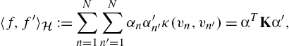
where α′:=[α′1,…,α′N]T![]() and the reproducing property has been employed that suggests 〈κ(⋅,vn0),κ(⋅,vn′0)〉H=iTn0Kin′0=κ(vn0,vn′0)
and the reproducing property has been employed that suggests 〈κ(⋅,vn0),κ(⋅,vn′0)〉H=iTn0Kin′0=κ(vn0,vn′0)![]() . The RKHS norm is defined by
. The RKHS norm is defined by
‖f‖2H:=〈f,f〉H=αTKα
and will be used as a regularizer to control overfitting and to cope with the under-determined reconstruction problem. As a special case, setting K=IN![]() recovers the standard inner product 〈f,f′〉H=fTf′
recovers the standard inner product 〈f,f′〉H=fTf′![]() and the Euclidean norm ‖f‖2H=‖f‖22
and the Euclidean norm ‖f‖2H=‖f‖22![]() . Note that when K≻0
. Note that when K≻0![]() , the set of functions of the form (8.3) coincides with RN
, the set of functions of the form (8.3) coincides with RN![]() .
.
Given {ys}Ss=1![]() , RKHS-based function estimators are obtained by solving functional minimization problems formulated as (see also, e.g., [18–20])
, RKHS-based function estimators are obtained by solving functional minimization problems formulated as (see also, e.g., [18–20])
ˆf:=argminf∈HL(y,ˉf)+μΩ(‖f‖H),
where the loss L![]() measures how the estimated function f at the observed vertices {vns}Ss=1
measures how the estimated function f at the observed vertices {vns}Ss=1![]() , collected in ˉf:=[f(vn1),…,f(vnS)]T=Sf
, collected in ˉf:=[f(vn1),…,f(vnS)]T=Sf![]() , deviates from the data y. The so-called square loss L(y,ˉf):=(1/S)∑Ss=1[ys−f(vns)]2
, deviates from the data y. The so-called square loss L(y,ˉf):=(1/S)∑Ss=1[ys−f(vns)]2![]() constitutes a popular choice for L
constitutes a popular choice for L![]() . The increasing function Ω is used to promote smoothness with typical choices including Ω(ζ)=|ζ|
. The increasing function Ω is used to promote smoothness with typical choices including Ω(ζ)=|ζ|![]() and Ω(ζ)=ζ2
and Ω(ζ)=ζ2![]() . The regularization parameter μ>0
. The regularization parameter μ>0![]() controls overfitting. Substituting (8.3) and (8.5) into (8.6) shows that ˆf
controls overfitting. Substituting (8.3) and (8.5) into (8.6) shows that ˆf![]() can be found as
can be found as
ˆα:=argminα∈RNL(y,SKα)+μΩ((αTKα)1/2),
ˆf=Kˆα.
An alternative form of (8.5) that will be frequently used in the sequel results upon noting that
αTKα=αTKK†Kα=fTK†f.
Thus, one can rewrite (8.6) as
ˆf:=argminf∈R{K}L(y,Sf)+μΩ((fTK†f)1/2).
Although graph signals can be reconstructed from (8.7), such an approach involves optimizing over N variables. Thankfully, the solution can be obtained by solving an optimization problem in S variables (where typically S≪N![]() ), by invoking the so-called representer theorem [19,21].
), by invoking the so-called representer theorem [19,21].
The representer theorem plays an instrumental role in the traditional infinite-dimensional setting where (8.6) cannot be solved directly; however, even when H![]() comprises graph signals, it can still be beneficial to reduce the dimension of the optimization in (8.7). The theorem essentially asserts that the solution to the functional minimization in (8.6) can be expressed as
comprises graph signals, it can still be beneficial to reduce the dimension of the optimization in (8.7). The theorem essentially asserts that the solution to the functional minimization in (8.6) can be expressed as
ˆf(v)=S∑s=1ˉαsκ(v,vns)
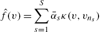
for some ˉαs∈R![]() , s=1,…,S
, s=1,…,S![]() .
.
The representer theorem shows the form of ˆf![]() , but does not provide the optimal {ˉαs}Ss=1
, but does not provide the optimal {ˉαs}Ss=1![]() , which are found after substituting (8.10) into (8.6) and solving the resulting optimization problem with respect to these coefficients. To this end, let ˉα:=[ˉα1,…,ˉαS]T
, which are found after substituting (8.10) into (8.6) and solving the resulting optimization problem with respect to these coefficients. To this end, let ˉα:=[ˉα1,…,ˉαS]T![]() and write α=STˉα
and write α=STˉα![]() to deduce that
to deduce that
ˆf=Kα=KSTˉα.
With ˉK:=SKST![]() and using (8.7) and (8.11), the optimal ˉα
and using (8.7) and (8.11), the optimal ˉα![]() can be found as
can be found as
ˆˉα:=argminˉα∈RSL(y,ˉKˉα)+μΩ((ˉαTˉKˉα)1/2).
Kernel ridge regression. For L![]() chosen as the square loss and Ω(ζ)=ζ2
chosen as the square loss and Ω(ζ)=ζ2![]() , the ˆf
, the ˆf![]() in (8.6) is referred to as the kernel ridge regression (RR) estimate [18]. If ˉK
in (8.6) is referred to as the kernel ridge regression (RR) estimate [18]. If ˉK![]() is full-rank, this estimate is given by ˆfRR=KSTˆˉα
is full-rank, this estimate is given by ˆfRR=KSTˆˉα![]() , where
, where
ˆˉα:=argminˉα∈RS1S‖y−ˉKˉα‖2+μˉαTˉKˉα
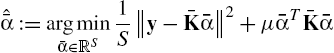
=(ˉK+μSIS)−1y.
Therefore, ˆfRR![]() can be expressed as
can be expressed as
ˆfRR=KST(ˉK+μSIS)−1y.
Section 8.2.2 shows that (8.14) generalizes a number of existing signal reconstructors upon properly selecting K.
8.2.2 Kernels on Graphs
When estimating functions on graphs, conventional kernels such as the Gaussian kernel cannot be adopted because the underlying set where graph signals are defined is not a metric space. Indeed, no vertex addition vn+vn′![]() , scaling βvn
, scaling βvn![]() or norm ‖vn‖
or norm ‖vn‖![]() can be naturally defined on V
can be naturally defined on V![]() . An alternative is to embed V
. An alternative is to embed V![]() into Euclidean space via a feature map ϕ:V→RD
into Euclidean space via a feature map ϕ:V→RD![]() and invoke a conventional kernel afterwards. However, for a given graph it is generally unclear how to explicitly design ϕ or select D. This motivates the adoption of kernels on graphs [3].
and invoke a conventional kernel afterwards. However, for a given graph it is generally unclear how to explicitly design ϕ or select D. This motivates the adoption of kernels on graphs [3].
A common approach to designing kernels on graphs is to apply a transformation function on the graph Laplacian [3]. The term Laplacian kernel comprises a wide family of kernels obtained by applying a certain function r(⋅)![]() to the Laplacian matrix L. Laplacian kernels are well motivated since they constitute the graph counterpart of the so-called translation-invariant kernels in Euclidean spaces [3]. This section reviews Laplacian kernels, provides beneficial insights in terms of interpolating signals and highlights their versatility in capturing information about the graph Fourier transform of the estimated signal.
to the Laplacian matrix L. Laplacian kernels are well motivated since they constitute the graph counterpart of the so-called translation-invariant kernels in Euclidean spaces [3]. This section reviews Laplacian kernels, provides beneficial insights in terms of interpolating signals and highlights their versatility in capturing information about the graph Fourier transform of the estimated signal.
The reason why the graph Laplacian constitutes one of the prominent candidates for regularization on graphs becomes clear upon recognizing that
fTLf=12∑(n,n′)∈EAn,n′(fn−fn′)2,
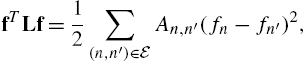
where An,n′![]() denotes weight associated with edge (n,n′)
denotes weight associated with edge (n,n′)![]() . The quadratic form of (8.15) becomes larger when function values vary a lot among connected vertices and therefore quantifies the smoothness of f on G
. The quadratic form of (8.15) becomes larger when function values vary a lot among connected vertices and therefore quantifies the smoothness of f on G![]() .
.
Let 0=λ1⩽λ2⩽…⩽λN![]() denote the eigenvalues of the graph Laplacian matrix L and consider the eigendecomposition L=UΛUT
denote the eigenvalues of the graph Laplacian matrix L and consider the eigendecomposition L=UΛUT![]() , where Λ:=diag{λ1,…,λN}
, where Λ:=diag{λ1,…,λN}![]() . A Laplacian kernel matrix is defined by
. A Laplacian kernel matrix is defined by
K:=r†(L):=Ur†(Λ)UT,
where r(Λ)![]() is the result of applying a user-selected, scalar, nonnegative map r:R→R+
is the result of applying a user-selected, scalar, nonnegative map r:R→R+![]() to the diagonal entries of Λ. The selection of map r generally depends on desirable properties that the target function is expected to have. Table 8.1 summarizes some well-known examples arising for specific choices of r.
to the diagonal entries of Λ. The selection of map r generally depends on desirable properties that the target function is expected to have. Table 8.1 summarizes some well-known examples arising for specific choices of r.
Table 8.1
| Kernel name | Function | Parameters |
|---|---|---|
| Diffusion [2] |
r(λ)=exp{σ2λ/2}
|
σ 2 |
| p-step random walk [3] | r(λ)=(a−λ)−p | a ⩾ 2, p ≥ 0 |
| Regularized Laplacian [3,22] | r(λ)=1 + σ2λ | σ 2 |
| Bandlimited [23] |
r(λ)={1/β,λ⩽λmax,β,otherwise
|
β > 0, λmax |
At this point, it is prudent to offer interpretations and insights on the operation of Laplacian kernels. Towards this objective, note first that the regularizer from (8.9) is an increasing function of
αTKα=αTKK†Kα=fTK†f=fTUr(Λ)UTf=ˇfTr(Λ)ˇf=N∑n=1r(λn)|ˇfn|2,

where ˇf:=UTf:=[ˇf1,…,ˇfN]T![]() comprises the projections of f onto the eigenspace of L and is referred to as the graph Fourier transform of f in the SPoG parlance [4]. Consequently, {ˇfn}Nn=1
comprises the projections of f onto the eigenspace of L and is referred to as the graph Fourier transform of f in the SPoG parlance [4]. Consequently, {ˇfn}Nn=1![]() are called frequency components. The so-called bandlimited (BL) functions in SPoG refer to those whose frequency components only exist inside some band B, that is, ˇfn=0,∀n>B
are called frequency components. The so-called bandlimited (BL) functions in SPoG refer to those whose frequency components only exist inside some band B, that is, ˇfn=0,∀n>B![]() .
.
By adopting the aforementioned SPoG notions, one can intuitively interpret the role of BL kernels. Indeed, it follows from (8.17) that the regularizer strongly penalizes those ˇfn![]() for which the corresponding r(λn)
for which the corresponding r(λn)![]() is large, thus promoting a specific structure in this “frequency” domain. Specifically, one prefers r(λn)
is large, thus promoting a specific structure in this “frequency” domain. Specifically, one prefers r(λn)![]() to be large whenever |ˇfn|2
to be large whenever |ˇfn|2![]() is small and vice versa. The fact that |ˇfn|2
is small and vice versa. The fact that |ˇfn|2![]() is expected to decrease with n for smooth f motivates the adoption of an increasing function r [3]. From (8.17) it is clear that r(λn)
is expected to decrease with n for smooth f motivates the adoption of an increasing function r [3]. From (8.17) it is clear that r(λn)![]() determines how heavily ˇfn
determines how heavily ˇfn![]() is penalized. Therefore, by setting r(λn)
is penalized. Therefore, by setting r(λn)![]() to be small when n⩽B
to be small when n⩽B![]() and extremely large when n>B
and extremely large when n>B![]() , one can expect the result to be a BL signal.
, one can expect the result to be a BL signal.
Observe that Laplacian kernels can capture forms of prior information richer than bandlimitedness [11,13,16,17] by selecting function r accordingly. For instance, using r(λ)=exp{σ2λ/2}![]() (diffusion kernel) accounts not only for smoothness of f as in (8.15), but also for the prior knowledge that f is generated by a process diffusing over the graph. Similarly, the use of r(λ)=(α−λ)−1
(diffusion kernel) accounts not only for smoothness of f as in (8.15), but also for the prior knowledge that f is generated by a process diffusing over the graph. Similarly, the use of r(λ)=(α−λ)−1![]() (1-step random walk) can accommodate cases where the signal captures a notion of network centrality.2
(1-step random walk) can accommodate cases where the signal captures a notion of network centrality.2
So far, f has been assumed deterministic, which precludes accommodating certain forms of prior information that probabilistic models can capture, such as domain knowledge and historical data. Suppose without loss of generality that {f(vn)}Nn=1![]() are zero mean random variables. The LMMSE estimator of f given y in (8.1) is the linear estimator ˆfLMMSE
are zero mean random variables. The LMMSE estimator of f given y in (8.1) is the linear estimator ˆfLMMSE![]() minimizing E‖f−ˆfLMMSE‖22
minimizing E‖f−ˆfLMMSE‖22![]() , where the expectation is over all f and noise realizations. With C:=E[ffT]
, where the expectation is over all f and noise realizations. With C:=E[ffT]![]() , the LMMSE estimate is
, the LMMSE estimate is
ˆfLMMSE=CST[SCST+σ2eIS]−1y,
where σ2e:=(1/S)E[‖e‖22]![]() denotes the noise variance. Comparing (8.18) with (8.14) and recalling that ˉK:=SKST
denotes the noise variance. Comparing (8.18) with (8.14) and recalling that ˉK:=SKST![]() , it follows that ˆfLMMSE=ˆfRR
, it follows that ˆfLMMSE=ˆfRR![]() if μS=σ2e
if μS=σ2e![]() and K=C
and K=C![]() . In other words, the similarity measure κ(vn,vn′)
. In other words, the similarity measure κ(vn,vn′)![]() embodied in such a kernel map is just the covariance cov[f(vn),f(vn′)]
embodied in such a kernel map is just the covariance cov[f(vn),f(vn′)]![]() . A related observation was pointed out in [27] for general kernel methods.
. A related observation was pointed out in [27] for general kernel methods.
In short, one can interpret kernel ridge regression as the LMMSE estimator of a signal f with covariance matrix equal to K; see also [28]. The LMMSE interpretation also suggests the usage of C as a kernel matrix, which enables signal reconstruction even when the graph topology is unknown. Although this discussion hinges on kernel ridge regression after setting K=C![]() , any other kernel estimator of the form (8.7) can benefit from vertex covariance kernels too.
, any other kernel estimator of the form (8.7) can benefit from vertex covariance kernels too.
8.2.3 Selecting Kernels From a Dictionary
The selection of the pertinent kernel matrix is of paramount importance to the performance of kernel-based methods [23,29]. This section presents an MKL approach that effects kernel selection in graph signal reconstruction. Two algorithms with complementary strengths will be presented. Both rely on a user-specified kernel dictionary, and the best kernel is built from the dictionary in a data-driven way.
The first algorithm, which we call RKHS superposition, is motivated by the fact that one specific H![]() in (8.6) is determined by some κ; therefore, kernel selection is tantamount to RKHS selection. Consequently, a kernel dictionary {κm}Mm=1
in (8.6) is determined by some κ; therefore, kernel selection is tantamount to RKHS selection. Consequently, a kernel dictionary {κm}Mm=1![]() gives rise to an RKHS dictionary {Hm}Mm=1
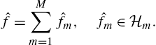
gives rise to an RKHS dictionary {Hm}Mm=1![]() , which motivates estimates of the form3
, which motivates estimates of the form3
ˆf=M∑m=1ˆfm,ˆfm∈Hm.
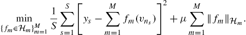
Upon adopting a criterion that controls sparsity in this expansion, the “best” RKHSs will be selected. A reasonable approach is therefore to generalize (8.6) to accommodate multiple RKHSs. With L![]() selected to be the square loss and Ω(ζ)=|ζ|
selected to be the square loss and Ω(ζ)=|ζ|![]() , one can pursue an estimate ˆf
, one can pursue an estimate ˆf![]() by solving
by solving
min{fm∈Hm}Mm=11SS∑s=1[ys−M∑m=1fm(vns)]2+μM∑m=1‖fm‖Hm.
Invoking the representer theorem per fm![]() establishes that the minimizers of (8.20) can be written as
establishes that the minimizers of (8.20) can be written as
ˆfm(v)=S∑s=1ˉαmsκm(v,vns),m=1,…,M
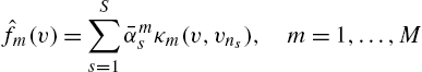
for some coefficients ˉαms![]() . Substituting (8.21) into (8.20) suggests obtaining these coefficients as
. Substituting (8.21) into (8.20) suggests obtaining these coefficients as
argmin{ˉαm}Mm=11S‖y−M∑m=1ˉKmˉαm‖2+μM∑m=1(ˉαTmˉKmˉαm)1/2,
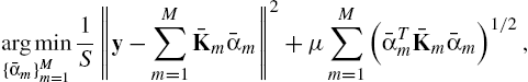
where ˉαm:=[ˉαm1,…,ˉαmS]T![]() and ˉKm:=SKmST
and ˉKm:=SKmST![]() with (Km)n,n′:=κm(vn,vn′)
with (Km)n,n′:=κm(vn,vn′)![]() . Letting ˇˉαm:=ˉK1/2mˉαm
. Letting ˇˉαm:=ˉK1/2mˉαm![]() , Eq. (8.22) becomes
, Eq. (8.22) becomes
argmin{ˇˉαm}Mm=11S‖y−M∑m=1ˉK1/2mˇˉαm‖2+μM∑m=1‖ˇˉαm‖2.
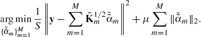
Interestingly, (8.23) can be efficiently solved using the alternating-direction method of multipliers (ADMM) [30,31] after some necessary reformulation [23].
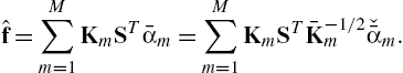
After obtaining {ˇˉαm}Mm=1![]() , the sought-after function estimate can be recovered as
, the sought-after function estimate can be recovered as
ˆf=M∑m=1KmSTˉαm=M∑m=1KmSTˉK−1/2mˇˉαm.
This MKL algorithm can identify the best subset of RKHSs—and therefore kernels—but entails MS unknowns (cf. (8.22)). Next, an alternative approach is discussed which can reduce the number of variables to M+S![]() at the price of not being able to assure a sparse kernel expansion.
at the price of not being able to assure a sparse kernel expansion.
The alternative approach is to postulate a kernel of the form K(θ)=∑Mm=1θmKm![]() , where {Km}Mm=1
, where {Km}Mm=1![]() is given and θm⩾0∀m
is given and θm⩾0∀m![]() . The coefficients θ:=[θ1,…,θM]T
. The coefficients θ:=[θ1,…,θM]T![]() can be found by jointly minimizing (8.12) with respect to θ and ˉα
can be found by jointly minimizing (8.12) with respect to θ and ˉα![]() [32]. We have
[32]. We have
(θ,ˆˉα):=argminθ,ˉα1SL(v,y,ˉK(θ)ˉα)+μΩ((ˉαTˉK(θ)ˉα)1/2),
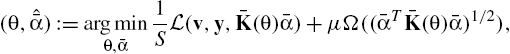
where ˉK(θ):=SK(θ)ST![]() . Except for degenerate cases, problem (8.25) is not jointly convex in θ and ˆˉα
. Except for degenerate cases, problem (8.25) is not jointly convex in θ and ˆˉα![]() , but it is separately convex in each vector for a convex L
, but it is separately convex in each vector for a convex L![]() [32]. Iterative algorithms for solving (8.23) and (8.25) are available in [23].
[32]. Iterative algorithms for solving (8.23) and (8.25) are available in [23].
8.2.4 Semiparametric Reconstruction
The approaches discussed so far are applicable to various problems but they are certainly limited by the modeling assumptions they make. In particular, the performance of algorithms belonging to the parametric family [11,15,33] is restricted by how well the signals actually adhere to the selected model. Nonparametric models, on the other hand [2,3,6,34], offer flexibility and robustness but they cannot readily incorporate information available a priori.
In practice however, it is not uncommon that neither of these approaches alone suffices for reliable inference. Consider, for instance, an employment-oriented social network such as LinkedIn, and suppose the goal is to estimate the salaries of all users given information about the salaries of a few. Clearly, besides network connections, exploiting available information regarding the users' education level and work experience could benefit the reconstruction task. The same is true in problems arising in link analysis, where the exploitation of hierarchical web structure can aid the task of estimating the importance of web pages [35]. In recommender systems, inferring preference scores for every item, given the users' feedback about particular items, could be cast as a signal reconstruction problem over the item correlation graph. Data sparsity imposes severe limitations on the quality of pure collaborative filtering methods [64]. Exploiting side information about the items is known to alleviate such limitations [36], leading to considerably improved recommendation performance [37,38].
A promising direction to endow nonparametric methods with prior information relies on a semiparametric approach whereby the signal of interest is modeled as the superposition of a parametric and a nonparametric component [39]. While the former leverages side information, the latter accounts for deviations from the parametric part and can also promote smoothness using kernels on graphs. In this section we outline two simple and reliable semiparametric estimators with complementary strengths, as detailed in [39].
8.2.4.1 Semiparametric Inference
Function f is modeled as the superposition4
/f=fP+fNP,
where fP:=[fP(v1),…,fP(vN)]T![]() and fNP:=[fNP(v1)
and fNP:=[fNP(v1)![]() , …,fNP(vN)]T
, …,fNP(vN)]T![]() .
.
The parametric term fP(v):=∑Mm=1βmbm(v)![]() captures the known signal structure via the basis B:={bm}Mm=1
captures the known signal structure via the basis B:={bm}Mm=1![]() , while the nonparametric term fNP
, while the nonparametric term fNP![]() belongs to an RKHS H
belongs to an RKHS H![]() , which accounts for deviations from the span of B
, which accounts for deviations from the span of B![]() . The goal of this section is to provide an efficient and reliable estimation of f given y, S, B
. The goal of this section is to provide an efficient and reliable estimation of f given y, S, B![]() , H
, H![]() and G
and G![]() .
.
Since fNP∈H![]() , vector fNP
, vector fNP![]() can be represented as in (8.3). By defining β:=[β1,…,βM]T
can be represented as in (8.3). By defining β:=[β1,…,βM]T![]() and the N×M
and the N×M![]() matrix B with entries (B)n,m:=bm(vn)
matrix B with entries (B)n,m:=bm(vn)![]() , the parametric term can be written in vector form as fP:=Bβ
, the parametric term can be written in vector form as fP:=Bβ![]() . The semiparametric estimates can be found as the solution of the following optimization problem:
. The semiparametric estimates can be found as the solution of the following optimization problem:
{ˆα,ˆβ}=argminα,β1SS∑s=1L(ys,f(vns))+μ‖fNP‖2Hs.t.f=Bβ+Kα,
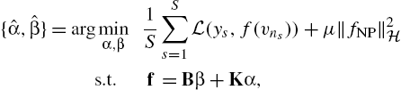
where the fitting loss L![]() quantifies the deviation of f from the data and μ>0
quantifies the deviation of f from the data and μ>0![]() is the regularization scalar that controls overfitting of the nonparametric term. Using (8.27), the semiparametric estimates are expressed as ˆf=Bˆβ+Kˆα
is the regularization scalar that controls overfitting of the nonparametric term. Using (8.27), the semiparametric estimates are expressed as ˆf=Bˆβ+Kˆα![]() .
.
Solving (8.27) entails minimization over N+M![]() variables. Clearly, when dealing with large-scale graphs this could lead to prohibitively large computational costs. To reduce complexity, the semiparametric version of the representer theorem [18,19] is employed, which establishes that
variables. Clearly, when dealing with large-scale graphs this could lead to prohibitively large computational costs. To reduce complexity, the semiparametric version of the representer theorem [18,19] is employed, which establishes that
ˆf=Bˆβ+KSTˆˉα,
where ˆˉα:=[ˆˉα1,…,ˆˉαS]T![]() . Estimates ˆˉα,ˆβ
. Estimates ˆˉα,ˆβ![]() are found as
are found as
{ˆˉα,ˆβ}=argminˉα,β1SS∑s=1L(ys,f(vns))+μ‖fNP‖2Hs.t.f=Bβ+KSTˉα,
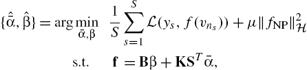
where ˉα:=[ˉα1,…,ˉαS]T![]() . The RKHS norm in (8.29) is expressed as ‖fNP‖2H=ˉαTˉKˉα
. The RKHS norm in (8.29) is expressed as ‖fNP‖2H=ˉαTˉKˉα![]() , with ˉK:=SKST
, with ˉK:=SKST![]() . Relative to (8.27), the number of optimization variables in (8.29) is reduced to the more affordable S+M
. Relative to (8.27), the number of optimization variables in (8.29) is reduced to the more affordable S+M![]() , with S≪N
, with S≪N![]() .
.
Next, two loss functions with complementary benefits will be considered: the square loss and the ϵ-insensitive loss. The square loss function is
L(ys,f(vns)):=‖ys−f(vns))‖22
and (8.29) admits the following closed-form solution:
ˆˉα=(PˉK+μIS)−1Py,
ˆβ=(ˉBTˉB)−1ˉBT(y−ˉKˆˉα),
where ˉB:=SB![]() , P:=IS−ˉB(ˉBTˉB)−1ˉBT
, P:=IS−ˉB(ˉBTˉB)−1ˉBT![]() . The complexity of (8.31) is O(S3+M3)
. The complexity of (8.31) is O(S3+M3)![]() .
.
The ϵ-insensitive loss function is given by
L(ys,f(vns)):=max(0,|ys−f(vns)|−ϵ),
where ϵ is tuned, e.g. via cross-validation, to minimize the generalization error and it has well-documented merits in signal estimation from quantized data [40]. Substituting (8.32) into (8.29) yields a convex nonsmooth quadratic problem that can be solved efficiently for ˉα![]() and β using, e.g., interior-point methods [18].
and β using, e.g., interior-point methods [18].
8.2.5 Numerical Tests
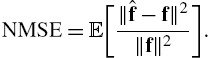
This section reports on the signal reconstruction performance of different methods using real as well as synthetic data. The performance of the estimators is assessed via Monte Carlo simulation by comparing the normalized mean square error (NMSE)
NMSE=E[‖ˆf−f‖2‖f‖2].
Multikernel reconstruction. The first data set contains departure and arrival information for flights among U.S. airports [41], from which 3×10⁶![]() flights in the months of July, August and September of 2014 and 2015 were selected. We construct a graph with N=50
flights in the months of July, August and September of 2014 and 2015 were selected. We construct a graph with N=50![]() vertices corresponding to the airports with highest traffic, and whenever the number of flights between the two airports exceeds 100 within the observation window, we connect the corresponding nodes with an edge.
vertices corresponding to the airports with highest traffic, and whenever the number of flights between the two airports exceeds 100 within the observation window, we connect the corresponding nodes with an edge.
A signal was constructed per day averaging the arrival delay of all inbound flights per selected airport. A total of 184 signals were considered, of which the first 154 were used for training (July, August, September 2014 and July, August 2015), and the remaining 30 for testing (September 2015). The weights of the edges between airports were learned using the training data based on the technique described in [23].
Table 8.2 lists the NMSE and the RMSE in minutes for the task of predicting the arrival delay at 40 airports when the delay at a randomly selected collection of 10 airports is observed. The second row corresponds to the ridge regression estimator that uses the nearly optimal estimated covariance kernel. The next two rows correspond to the multikernel approaches in §8.2.3 with a dictionary of 30 diffusion kernels with values of σ2![]() uniformly spaced between 0.1 and 7. The rest of the rows pertain to graph BL estimators. Table 8.2 demonstrates the reliable performance of covariance kernels as well as the herein discussed multikernel approaches relative to competing alternatives.
uniformly spaced between 0.1 and 7. The rest of the rows pertain to graph BL estimators. Table 8.2 demonstrates the reliable performance of covariance kernels as well as the herein discussed multikernel approaches relative to competing alternatives.
Table 8.2
| NMSE | RMSE[min] | |
|---|---|---|
| KRR with cov. kernel | 0.34 | 3.95 |
| Multikernel, RS | 0.44 | 4.51 |
| Multikernel, KS | 0.43 | 4.45 |
| BL for B=2 | 1.55 | 8.45 |
| BL for B=3 | 32.64 | 38.72 |
| BL, cut-off | 3.97 | 13.5 |
Semiparametric reconstruction. An Erdős–Rényi graph with probability of edge presence 0.6 and N=200![]() nodes was generated, and f was formed by superimposing a BL signal [13,15] plus a piece-wise constant signal [42]; that is,
nodes was generated, and f was formed by superimposing a BL signal [13,15] plus a piece-wise constant signal [42]; that is,
f=10∑i=1γiui+6∑i=1δi1Vc,
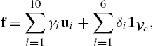
where {γi}10i=1![]() and {δi}6i=1
and {δi}6i=1![]() are standardized Gaussian distributed, {ui}10i=1
are standardized Gaussian distributed, {ui}10i=1![]() are the eigenvectors associated with the 10 smallest eigenvalues of the Laplacian matrix, {Vi}6i=1
are the eigenvectors associated with the 10 smallest eigenvalues of the Laplacian matrix, {Vi}6i=1![]() are the vertex sets of six clusters obtained via spectral clustering [43] and 1Vi
are the vertex sets of six clusters obtained via spectral clustering [43] and 1Vi![]() is the indicator vector with entries (1Vi)n:=1
is the indicator vector with entries (1Vi)n:=1![]() , if vn∈Vi
, if vn∈Vi![]() , and 0 otherwise. The parametric basis B={1Vi}6i=1
, and 0 otherwise. The parametric basis B={1Vi}6i=1![]() was used by the estimators capturing the prior knowledge, and S vertices were sampled uniformly at random. The subsequent experiments evaluate the performance of the semiparametric graph kernel estimators, SP-GK and SP-GK(ϵ), resulting from using (8.30) and (8.32) in (8.29), respectively; the parametric (P) that considers only the parametric term in (8.26), the nonparametric (NP) [2,3] that considers only the nonparametric term in (8.26) and the graph BL estimators from [13,15], which assume a BL model with bandwidth B. For all the experiments, the diffusion kernel (cf. Table 8.1) with parameter σ is employed. First, white Gaussian noise es
was used by the estimators capturing the prior knowledge, and S vertices were sampled uniformly at random. The subsequent experiments evaluate the performance of the semiparametric graph kernel estimators, SP-GK and SP-GK(ϵ), resulting from using (8.30) and (8.32) in (8.29), respectively; the parametric (P) that considers only the parametric term in (8.26), the nonparametric (NP) [2,3] that considers only the nonparametric term in (8.26) and the graph BL estimators from [13,15], which assume a BL model with bandwidth B. For all the experiments, the diffusion kernel (cf. Table 8.1) with parameter σ is employed. First, white Gaussian noise es![]() of variance σ2e
of variance σ2e![]() is added to each sample fs
is added to each sample fs![]() to yield the signal-to-noise ratio SNRe:=‖f‖22/(Nσ2e)
to yield the signal-to-noise ratio SNRe:=‖f‖22/(Nσ2e)![]() . Fig. 8.1B presents the NMSE of different methods. As expected, the limited flexibility of the parametric approaches, BL and P, affects their ability to capture the true signal structure. The NP estimator achieves smaller NMSE, but only when the amount of available samples is adequate. Both semiparametric estimators were found to outperform other approaches, exhibiting reliable reconstruction even with few samples.
. Fig. 8.1B presents the NMSE of different methods. As expected, the limited flexibility of the parametric approaches, BL and P, affects their ability to capture the true signal structure. The NP estimator achieves smaller NMSE, but only when the amount of available samples is adequate. Both semiparametric estimators were found to outperform other approaches, exhibiting reliable reconstruction even with few samples.
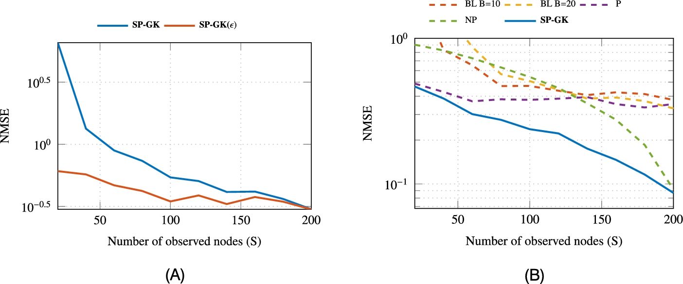
To illustrate the benefits of employing different loss functions (8.30) and (8.32), we compare the performance of SP-GK and SP-GK(ϵ) in the presence of outlying noise. Each sample fs![]() is contaminated with Gaussian noise os
is contaminated with Gaussian noise os![]() of large variance σ2o
of large variance σ2o![]() with probability p=0.1
with probability p=0.1![]() . Fig. 8.1A demonstrates the robustness of SP-GK(ϵ) which is attributed to the ϵ-insensitive loss function (8.32). Further experiments using real signals can be found in [39].
. Fig. 8.1A demonstrates the robustness of SP-GK(ϵ) which is attributed to the ϵ-insensitive loss function (8.32). Further experiments using real signals can be found in [39].
8.3 Inference of Dynamic Functions Over Dynamic Graphs
Networks that exhibit time varying connectivity patterns with time varying node attributes arise in a plethora of network science–related applications. Sometimes these dynamic network topologies switch between a finite number of discrete states, governed by sudden changes of the underlying dynamics [44,45]. A challenging problem that arises in this setting is that of reconstructing time evolving functions on graphs, given their values on a subset of vertices and time instants. Efficiently exploiting spatiotemporal dynamics can markedly impact sampling costs by reducing the number of vertices that need to be observed to attain a target performance. Such a reduction can be of paramount importance in certain applications, e.g., in monitoring time-dependent activity of different regions of the brain through invasive electrocorticography (ECoG), where observing a vertex requires the implantation of an intracranial electrode [44].
Although one could reconstruct a time varying function per time slot using the non- or semiparametric methods of §8.2, leveraging time correlations typically yields estimators with improved performance. Schemes tailored for time evolving functions on graphs include [46] and [47], which predict the function values at time t given observations up to time t−1![]() . However, these schemes assume that the function of interest adheres to a specific vector autoregressive model. Other works target time-invariant functions, but can only afford tracking sufficiently slow variations. This is the case with the dictionary learning approach in [48] and the distributed algorithms in [49] and [50]. Unfortunately, the flexibility of these algorithms to capture spatial information is also limited since [48] focuses on Laplacian regularization, whereas [49] and [50] require the signal to be BL.
. However, these schemes assume that the function of interest adheres to a specific vector autoregressive model. Other works target time-invariant functions, but can only afford tracking sufficiently slow variations. This is the case with the dictionary learning approach in [48] and the distributed algorithms in [49] and [50]. Unfortunately, the flexibility of these algorithms to capture spatial information is also limited since [48] focuses on Laplacian regularization, whereas [49] and [50] require the signal to be BL.
Motivated by the aforementioned limitations, in what comes next we extend the framework presented in §8.2 accommodating time varying function reconstruction over dynamic graphs. But before we delve into the time varying setting, a few definitions are in order.
Definitions: A time varying graph is a tuple G(t):=(V,At)![]() , where V:={v1,…,vN}
, where V:={v1,…,vN}![]() is the vertex set and At∈RN×N
is the vertex set and At∈RN×N![]() is the adjacency matrix at time t, whose (n,n′)
is the adjacency matrix at time t, whose (n,n′)![]() th entry An,n′(t)
th entry An,n′(t)![]() assigns a weight to the pair of vertices (vn,vn′)
assigns a weight to the pair of vertices (vn,vn′)![]() at time t. A time-invariant graph is a special case with At=At′∀t,t′
at time t. A time-invariant graph is a special case with At=At′∀t,t′![]() . Adopting common assumptions made in related literature (e.g., [1, Chapter 2], [4,9]), we also define G(t)
. Adopting common assumptions made in related literature (e.g., [1, Chapter 2], [4,9]), we also define G(t)![]() (i) to have nonnegative weights (An,n′(t)⩾0∀t, and ∀n≠n′
(i) to have nonnegative weights (An,n′(t)⩾0∀t, and ∀n≠n′![]() ), (ii) to have no self-edges (An,n(t)=0∀n,t
), (ii) to have no self-edges (An,n(t)=0∀n,t![]() ) and (iii) to be undirected (An,n′(t)=An′,n(t)∀n,n′,t
) and (iii) to be undirected (An,n′(t)=An′,n(t)∀n,n′,t![]() ).
).
A time varying function or signal on a graph is a map f:V×T→R![]() , where T:={1,2,…}
, where T:={1,2,…}![]() is the set of time indices. The value f(vn,t)
is the set of time indices. The value f(vn,t)![]() of f at vertex vn
of f at vertex vn![]() and time t can be thought of as the value of an attribute of vn∈V
and time t can be thought of as the value of an attribute of vn∈V![]() at time t. The values of f at time t will be collected in ft:=[f(v1,t),…,f(vN,t)]T
at time t. The values of f at time t will be collected in ft:=[f(v1,t),…,f(vN,t)]T![]() .
.
At time t, vertices with indices in the time-dependent set St:={n1(t),…,nS(t)(t)}![]() , 1⩽n1(t)<⋯<nS(t)(t)⩽N
, 1⩽n1(t)<⋯<nS(t)(t)⩽N![]() , are observed. The resulting samples can be expressed as ys(t)=f(vns(t),t)+es(t),s=1,…,S(t)
, are observed. The resulting samples can be expressed as ys(t)=f(vns(t),t)+es(t),s=1,…,S(t)![]() , where es(t)
, where es(t)![]() models the observation error. By letting yt:=[y1(t),…,yS(t)(t)]T
models the observation error. By letting yt:=[y1(t),…,yS(t)(t)]T![]() , the observations can be conveniently expressed as
, the observations can be conveniently expressed as
yt=Stft+et,t=1,2,…,
where et:=[e1(t),…,eS(t)(t)]T![]() and the S(t)×N
and the S(t)×N![]() sampling matrix St
sampling matrix St![]() contains ones at positions (s,ns(t))
contains ones at positions (s,ns(t))![]() , s=1,…,S(t)
, s=1,…,S(t)![]() and zeros elsewhere.
and zeros elsewhere.
The broad goal of this section is to “reconstruct” f from the observations {yt}t![]() in (8.35). Two formulations will be considered.
in (8.35). Two formulations will be considered.
Batch formulation. In the batch reconstruction problem, one aims at finding {ft}Tt=1![]() given {G(t)}Tt=1
given {G(t)}Tt=1![]() , the sample locations {St}Tt=1
, the sample locations {St}Tt=1![]() and all observations {yt}Tt=1
and all observations {yt}Tt=1![]() .
.
Online formulation. At every time t, one is given G![]() together with St
together with St![]() and yt
and yt![]() , and the goal is to find ft
, and the goal is to find ft![]() . The latter can be obtained possibly based on a previous estimate of ft−1
. The latter can be obtained possibly based on a previous estimate of ft−1![]() , but the complexity per time slot t must be independent of t.
, but the complexity per time slot t must be independent of t.
To solve these problems, we will rely on the assumption that f evolves smoothly over space and time, yet more structured dynamics can be incorporated if known.
8.3.1 Kernels on Extended Graphs
This section extends the kernel-based learning framework of §8.2 to subsume time evolving functions over possibly dynamic graphs through the notion of graph extension, by which the time dimension receives the same treatment as the spatial dimension. The versatility of kernel-based methods to leverage spatial information [23] is thereby inherited and broadened to account for temporal dynamics as well. This vantage point also accommodates time varying sampling sets and topologies.
8.3.1.1 Extended Graphs
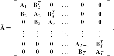
An immediate approach to reconstructing time evolving functions is to apply (8.9) separately for each t=1,…,T![]() . This yields the instantaneous estimator (IE)
. This yields the instantaneous estimator (IE)
ˆf(IE)t:=argminf1S(t)‖yt−Stf‖22+μfTK†tf.
Unfortunately, this estimator does not account for the possible relation between, e.g., f(vn,t)![]() and f(vn,t−1)
and f(vn,t−1)![]() . If, for instance, f varies slowly over time, an estimate of f(vn,t)
. If, for instance, f varies slowly over time, an estimate of f(vn,t)![]() may as well benefit from leveraging observations ys(τ)
may as well benefit from leveraging observations ys(τ)![]() at time instants τ≠t
at time instants τ≠t![]() . Exploiting temporal dynamics potentially reduces the number of vertices that have to be sampled to attain a target reconstruction performance, which in turn can markedly reduce sampling costs.
. Exploiting temporal dynamics potentially reduces the number of vertices that have to be sampled to attain a target reconstruction performance, which in turn can markedly reduce sampling costs.
Incorporating temporal dynamics into kernel-based reconstruction, which can only handle a single snapshot (cf. §8.2), necessitates an appropriate reformulation of time evolving function reconstruction as a problem of reconstructing a time-invariant function. An appealing possibility is to replace G![]() with its extended version ˜G:=(˜V,˜A)
with its extended version ˜G:=(˜V,˜A)![]() , where each vertex in V
, where each vertex in V![]() is replicated T times to yield the extended vertex set ˜V:={vn(t),n=1,…,N,t=1,…,T}
is replicated T times to yield the extended vertex set ˜V:={vn(t),n=1,…,N,t=1,…,T}![]() , and the (n+N(t−1),n′+N(t′−1))
, and the (n+N(t−1),n′+N(t′−1))![]() th entry of the TN×TN
th entry of the TN×TN![]() extended adjacency matrix ˜A
extended adjacency matrix ˜A![]() equals the weight of the edge (vn(t),vn′(t′))
equals the weight of the edge (vn(t),vn′(t′))![]() . The time varying function f can thus be replaced with its extended time-invariant counterpart ˜f:˜V→R
. The time varying function f can thus be replaced with its extended time-invariant counterpart ˜f:˜V→R![]() with ˜f(vn(t))=f(vn,t)
with ˜f(vn(t))=f(vn,t)![]() .
.
Definition 1
Let V:={v1,…,vN}![]() denote a vertex set and let G:=(V,{At}Tt=1)
denote a vertex set and let G:=(V,{At}Tt=1)![]() be a time varying graph. A graph ˜G
be a time varying graph. A graph ˜G![]() with vertex set ˜V:={vn(t),n=1,…,N,t=1,…,T}
with vertex set ˜V:={vn(t),n=1,…,N,t=1,…,T}![]() and NT×NT
and NT×NT![]() adjacency matrix ˜A
adjacency matrix ˜A![]() is an extended graph of G
is an extended graph of G![]() if the tth N×N
if the tth N×N![]() diagonal block of ˜A
diagonal block of ˜A![]() equals At
equals At![]() .
.
In general, the diagonal blocks {At}Tt=1![]() do not provide full description of the underlying extended graph. Indeed, one also needs to specify the off-diagonal block entries of ˜A
do not provide full description of the underlying extended graph. Indeed, one also needs to specify the off-diagonal block entries of ˜A![]() to capture the spatiotemporal dynamics of f.
to capture the spatiotemporal dynamics of f.
As an example, consider an extended graph with
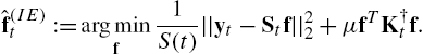
˜A=btridiag{A1,…,AT;B(T)2,…,B(T)T},
where B(T)t∈RN×N+![]() connects {vn(t−1)}Nn=1
connects {vn(t−1)}Nn=1![]() to {vn(t)}Nn=1
to {vn(t)}Nn=1![]() , t=2,…,T
, t=2,…,T![]() , and btridiag{A1
, and btridiag{A1![]() , …,AT;B2,…,BT}
, …,AT;B2,…,BT}![]() represents the symmetric block tridiagonal matrix
represents the symmetric block tridiagonal matrix
˜A=[A1BT20…00B2A2BT3…000B3A3…00⋮⋮⋮⋱⋮⋮000…AT−1BTT000…BTAT].
For instance, each vertex can be connected to its neighbors at the previous time instant by setting B(T)t=At−1![]() , or it can be connected to its replicas at adjacent time instants by setting B(T)t
, or it can be connected to its replicas at adjacent time instants by setting B(T)t![]() to be diagonal. Such a graph is depicted in Fig. 8.2.
to be diagonal. Such a graph is depicted in Fig. 8.2.
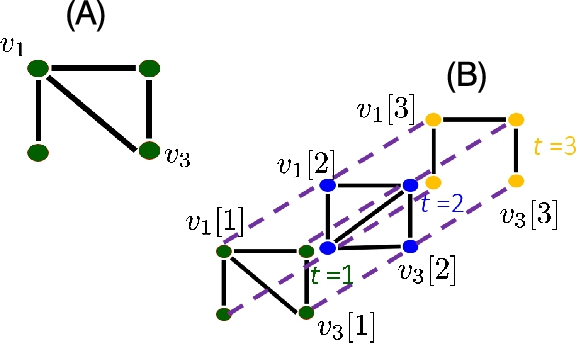
 for diagonal B(T)t
 . Edges connecting vertices at the same time instant are represented by solid lines whereas edges connecting vertices at different time instants are represented by dashed lines.
8.3.1.2 Batch and Online Reconstruction via Space–Time Kernels
The extended graph enables a generalization of the estimators in §8.2 for time evolving functions. The rest of this subsection discusses two such KRR estimators.
Consider first the batch formulation, where all the ˜S:=∑Tt=1St![]() samples in ˜y:=[yT1,…,yTT]T
samples in ˜y:=[yT1,…,yTT]T![]() are available, and the goal is to estimate ˜f:=[fT1,…,fTT]T
are available, and the goal is to estimate ˜f:=[fT1,…,fTT]T![]() . Directly applying the KRR criterion in (8.9) to reconstruct ˜f
. Directly applying the KRR criterion in (8.9) to reconstruct ˜f![]() on the extended graph ˜G
on the extended graph ˜G![]() yields
yields
ˆ˜f:=argmin˜f‖˜y−˜S˜f‖2D+μ˜fT˜K†˜f,
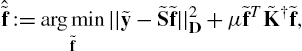
where ˜K![]() is now a TN×TN
is now a TN×TN![]() “space–time” kernel matrix, ˜S:=bdiag{S1,…,ST}
“space–time” kernel matrix, ˜S:=bdiag{S1,…,ST}![]() and D:=bdiag{S(1)IS(1),…,S(T)IS(T)}
and D:=bdiag{S(1)IS(1),…,S(T)IS(T)}![]() . If ˜K
. If ˜K![]() is invertible, (8.38a) can be solved in closed form as
is invertible, (8.38a) can be solved in closed form as
ˆ˜f=˜K˜ST(˜S˜K˜ST+μD)−1˜y.
The “space–time” kernel ˜K![]() , captures complex spatiotemporal dynamics. If the topology is time-invariant, ˜K
, captures complex spatiotemporal dynamics. If the topology is time-invariant, ˜K![]() can be specified in a bidimensional plane of spatiotemporal frequency similar to §8.2.2.5
can be specified in a bidimensional plane of spatiotemporal frequency similar to §8.2.2.5
In the online formulation, one aims to estimate ft![]() after the ˜S(t):=∑tτ=1S(τ)
after the ˜S(t):=∑tτ=1S(τ)![]() samples in ˜yt:=[yT1,…,yTt]T
samples in ˜yt:=[yT1,…,yTt]T![]() become available. Based on these samples, the KRR estimate of ˜f
become available. Based on these samples, the KRR estimate of ˜f![]() , denoted as ˆ˜f1:T|t
, denoted as ˆ˜f1:T|t![]() , is clearly
, is clearly
ˆ˜f1:T|t:=argmin˜f‖˜yt−˜St˜f‖2Dt+μ˜fT˜K−1˜f
=˜K˜STt(˜St˜K˜STt+μDt)−1˜yt,
where ˜K![]() is assumed invertible for simplicity, Dt:=bdiag{S(1)IS(1),…,S(t)IS(t)}
is assumed invertible for simplicity, Dt:=bdiag{S(1)IS(1),…,S(t)IS(t)}![]() and ˜St:=[diag{S1,…,St},0˜S(t)×(T−t)N]∈{0,1}˜S(t)×TN
and ˜St:=[diag{S1,…,St},0˜S(t)×(T−t)N]∈{0,1}˜S(t)×TN![]() .
.
The estimate in (8.39) comprises the per slot estimates {ˆfτ|t}Tτ=1![]() ; that is, ˆ˜f1:T|t:=[ˆfT1|t,…,ˆfTT|t]T
; that is, ˆ˜f1:T|t:=[ˆfT1|t,…,ˆfTT|t]T![]() with ˆfτ|t:=[ˆf1(τ|t),…,ˆfN(τ|t)]T
with ˆfτ|t:=[ˆf1(τ|t),…,ˆfN(τ|t)]T![]() , where ˆfτ|t
, where ˆfτ|t![]() (respectively ˆfn(τ|t)
(respectively ˆfn(τ|t)![]() ) is the KRR estimate of fτ
) is the KRR estimate of fτ![]() (f(vn,τ)
(f(vn,τ)![]() ) given the observations up to time t. With this notation, it follows that for all t,τ
) given the observations up to time t. With this notation, it follows that for all t,τ![]()
ˆfτ|t=(iTT,τ⊗IN)ˆ˜f1:T|t.
Regarding t as the present, (8.39) therefore provides estimates of past, present and future values of f. The solution to the online problem comprises the sequence of present KRR estimates for all t, that is, {ˆft|t}Tt=1![]() . This can be obtained by solving (8.39a) in closed form per t as in (8.39b) and then applying (8.40). However, such an approach does not yield a desirable online algorithm since its complexity per time slot is O(˜S3(t))
. This can be obtained by solving (8.39a) in closed form per t as in (8.39b) and then applying (8.40). However, such an approach does not yield a desirable online algorithm since its complexity per time slot is O(˜S3(t))![]() and therefore increasing with t. For this reason, this approach is not satisfactory since the online problem formulation requires the complexity per time slot of the desired algorithm to be independent of t. An algorithm that does satisfy this requirement yet provides the exact KRR estimate is presented next when the kernel matrix is any positive definite matrix ˜K
and therefore increasing with t. For this reason, this approach is not satisfactory since the online problem formulation requires the complexity per time slot of the desired algorithm to be independent of t. An algorithm that does satisfy this requirement yet provides the exact KRR estimate is presented next when the kernel matrix is any positive definite matrix ˜K![]() satisfying
satisfying
˜K−1=btridiag{D1,…,DT;C2,…,CT}
for some N×N![]() matrices {Dt}Tt=1
matrices {Dt}Tt=1![]() and {Ct}Tt=2
and {Ct}Tt=2![]() . Kernels in this important family are designed in [51].
. Kernels in this important family are designed in [51].
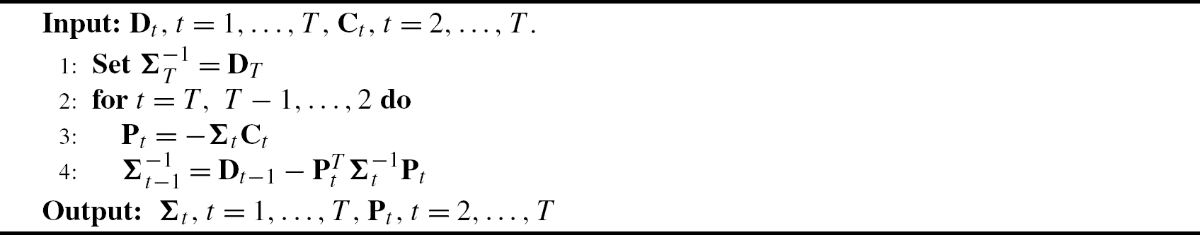
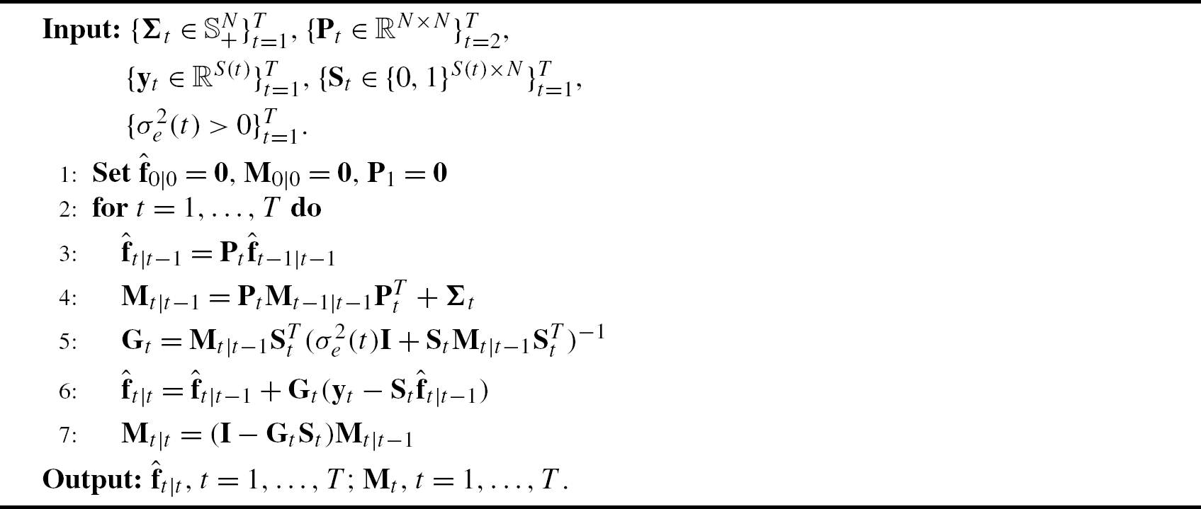
If ˜K![]() is of the form (8.41), then the kernel Kalman filter (KKF) in Algorithm 2 returns the sequence {ˆft|t}Tt=1
is of the form (8.41), then the kernel Kalman filter (KKF) in Algorithm 2 returns the sequence {ˆft|t}Tt=1![]() , where ˆft|t
, where ˆft|t![]() is given by (8.40). The N×N
is given by (8.40). The N×N![]() matrices {Pτ}Tτ=2
matrices {Pτ}Tτ=2![]() and {Στ}Tτ=1
and {Στ}Tτ=1![]() are obtained offline by Algorithm 1, and σ2e(τ)=μS(τ)∀τ
are obtained offline by Algorithm 1, and σ2e(τ)=μS(τ)∀τ![]() .
.
The KKF generalizes the probabilistic KF since the latter is recovered upon setting ˜K![]() to be the covariance matrix of ˜f
to be the covariance matrix of ˜f![]() in the probabilistic KF. The assumptions made by the probabilistic KF are stronger than those involved in the KKF. Specifically, in the probabilistic KF, ft
in the probabilistic KF. The assumptions made by the probabilistic KF are stronger than those involved in the KKF. Specifically, in the probabilistic KF, ft![]() must adhere to a linear state space model, ft=Ptft−1+ηt
must adhere to a linear state space model, ft=Ptft−1+ηt![]() , with known transition matrix Pt
, with known transition matrix Pt![]() , where the state noise ηt
, where the state noise ηt![]() is uncorrelated over time and has known covariance matrix Σt
is uncorrelated over time and has known covariance matrix Σt![]() . Furthermore, the observation noise et
. Furthermore, the observation noise et![]() must be uncorrelated over time and have a known covariance matrix. Correspondingly, the performance guarantees of the probabilistic KF are also stronger: the resulting estimate is optimal in the mean square error sense among all linear estimators. Furthermore, if ηt
must be uncorrelated over time and have a known covariance matrix. Correspondingly, the performance guarantees of the probabilistic KF are also stronger: the resulting estimate is optimal in the mean square error sense among all linear estimators. Furthermore, if ηt![]() and yt
and yt![]() are jointly Gaussian, t=1,…,T
are jointly Gaussian, t=1,…,T![]() , then the probabilistic KF estimate is optimal in the mean square error sense among all (not necessarily linear) estimators. In contrast, the requirements of the proposed KKF are much weaker since they only specify that f must evolve smoothly with respect to a given extended graph. As expected, the performance guarantees are similarly weaker; see e.g. [18, Chapter 5]. However, since the KKF generalizes the probabilistic KF, the reconstruction performance of the former for judiciously selected ˜K
, then the probabilistic KF estimate is optimal in the mean square error sense among all (not necessarily linear) estimators. In contrast, the requirements of the proposed KKF are much weaker since they only specify that f must evolve smoothly with respect to a given extended graph. As expected, the performance guarantees are similarly weaker; see e.g. [18, Chapter 5]. However, since the KKF generalizes the probabilistic KF, the reconstruction performance of the former for judiciously selected ˜K![]() cannot be worse than the reconstruction performance of the latter for any given criterion. The caveat, however, is that such a selection is not necessarily easy.
cannot be worse than the reconstruction performance of the latter for any given criterion. The caveat, however, is that such a selection is not necessarily easy.
For the rigorous statement and proof relating the celebrated KF [52, Chapter 17] and the optimization problem in (8.39a), see [51]. Algorithm 2 requires O(N3)![]() operations per time slot, whereas the complexity of evaluating (8.39b) for the tth time slot is O(˜S3(t))
operations per time slot, whereas the complexity of evaluating (8.39b) for the tth time slot is O(˜S3(t))![]() , which increases with t and becomes eventually prohibitive. Since distributed versions of the Kalman filter are well studied [53], decentralized KKF algorithms can be pursued to further reduce the computational complexity.
, which increases with t and becomes eventually prohibitive. Since distributed versions of the Kalman filter are well studied [53], decentralized KKF algorithms can be pursued to further reduce the computational complexity.
8.3.2 Multikernel Kriged Kalman Filters
The following section applies the KRR framework presented in §8.2 to online data-adaptive estimators of ft![]() . Specifically, a spatiotemporal model is presented that judiciously captures the dynamics over space and time. Based on this model the KRR criterion over time and space is formulated, and an online algorithm is derived with affordable computational complexity, when the kernels are preselected. To bypass the need for selecting an appropriate kernel, this section discusses a data-adaptive multikernel learning extension of the KRR estimator that learns the optimal kernel “on-the-fly.”
. Specifically, a spatiotemporal model is presented that judiciously captures the dynamics over space and time. Based on this model the KRR criterion over time and space is formulated, and an online algorithm is derived with affordable computational complexity, when the kernels are preselected. To bypass the need for selecting an appropriate kernel, this section discusses a data-adaptive multikernel learning extension of the KRR estimator that learns the optimal kernel “on-the-fly.”
8.3.2.1 Spatiotemporal Models
Consider modeling the dynamics of ft![]() separately over time and space as f(vn,t)=f(ν)(vn,t)+f(χ)(vn,t)
separately over time and space as f(vn,t)=f(ν)(vn,t)+f(χ)(vn,t)![]() , or in vector form
, or in vector form
ft=f(ν)t+f(χ)t,
where f(ν)t:=[f(ν)(v1,t),…,f(ν)(vN,t)]T![]() and f(χ)t:=[f(χ)(v1,t),…,f(χ)(vN,t)]T
and f(χ)t:=[f(χ)(v1,t),…,f(χ)(vN,t)]T![]() . The first term {f(ν)t}t
. The first term {f(ν)t}t![]() captures only spatial dependencies and can be thought of as exogenous input to the graph that does not affect the evolution of the function in time.
captures only spatial dependencies and can be thought of as exogenous input to the graph that does not affect the evolution of the function in time.
The second term {f(χ)t}t![]() accounts for spatiotemporal dynamics. A popular approach [54, Chapter 3] models f(χ)t
accounts for spatiotemporal dynamics. A popular approach [54, Chapter 3] models f(χ)t![]() with the state equation
with the state equation
f(χ)t=At,t−1f(χ)t−1+ηt,t=1,2,…,
where At,t−1![]() is a generic transition matrix that can be chosen, e.g., as the N×N
is a generic transition matrix that can be chosen, e.g., as the N×N![]() adjacency of a possibly directed “transition graph,” with f(χ)0=0
adjacency of a possibly directed “transition graph,” with f(χ)0=0![]() and ηt∈RN
and ηt∈RN![]() capturing the state error. The state transition matrix At,t−1
capturing the state error. The state transition matrix At,t−1![]() can be selected in accordance with the prior information available. Simplicity in estimation is a major advantage of the random walk model [55], where At,t−1=αIN
can be selected in accordance with the prior information available. Simplicity in estimation is a major advantage of the random walk model [55], where At,t−1=αIN![]() with α>0
with α>0![]() . On the other hand, adherence to the graph prompts the selection At,t−1=αA
. On the other hand, adherence to the graph prompts the selection At,t−1=αA![]() , in which case (8.43) amounts to a diffusion process on the time-invariant graph G
, in which case (8.43) amounts to a diffusion process on the time-invariant graph G![]() . The recursion in (8.43) is a vector autoregressive model (VARM) of order one and offers flexibility in tracking multiple forms of temporal dynamics [54, Chapter 3]. The model in (8.43) captures the dependence between f(χ)(vn,t)
. The recursion in (8.43) is a vector autoregressive model (VARM) of order one and offers flexibility in tracking multiple forms of temporal dynamics [54, Chapter 3]. The model in (8.43) captures the dependence between f(χ)(vn,t)![]() and its time lagged versions {f(χ)(vn,t−1)}Nn=1
and its time lagged versions {f(χ)(vn,t−1)}Nn=1![]() .
.
Next, a model with increased flexibility is presented to account for instantaneous spatial dependencies as well. We have
f(χ)t=At,tf(χ)t+At,t−1f(χ)t−1+ηt,t=1,2,…,
where At,t![]() encodes the instantaneous relation between f(χ)(vn,t)
encodes the instantaneous relation between f(χ)(vn,t)![]() and {f(χ)(vn′,t)}n′≠n
and {f(χ)(vn′,t)}n′≠n![]() . The recursion in (8.44) amounts to a structural vector autoregressive model (SVARM) [44]. Interestingly, (8.44) can be rewritten as
. The recursion in (8.44) amounts to a structural vector autoregressive model (SVARM) [44]. Interestingly, (8.44) can be rewritten as
f(χ)t=(IN−At,t)−1At,t−1f(χ)t−1+(IN−At,t)−1ηt,
where IN−At,t![]() is assumed invertible. After defining ˜ηt:=(IN−At,t)−1ηt
is assumed invertible. After defining ˜ηt:=(IN−At,t)−1ηt![]() and ˜At,t−1:=(IN−At,t)−1At,t−1
and ˜At,t−1:=(IN−At,t)−1At,t−1![]() , (8.44) boils down to
, (8.44) boils down to
f(χ)t=˜At,t−1f(χ)t−1+˜ηt,
which is equivalent to (8.43). This section will focus on deriving estimators based on (8.43), but can also accommodate (8.44) using the aforementioned reformulation.
Modeling ft![]() as the superposition of a term f(χ)t
as the superposition of a term f(χ)t![]() , capturing the slow dynamics over time with a state space equation, and a term f(ν)t
, capturing the slow dynamics over time with a state space equation, and a term f(ν)t![]() accounting for fast dynamics is motivated by the application at hand [56,55,57]. In the kriging terminology [56], f(ν)t
accounting for fast dynamics is motivated by the application at hand [56,55,57]. In the kriging terminology [56], f(ν)t![]() is said to model small-scale spatial fluctuations, whereas f(χ)t
is said to model small-scale spatial fluctuations, whereas f(χ)t![]() captures the so-called trend. The decomposition (8.42) is often dictated by the sampling interval; while f(χ)t
captures the so-called trend. The decomposition (8.42) is often dictated by the sampling interval; while f(χ)t![]() captures slow dynamics relative to the sampling interval, fast variations are modeled with f(ν)t
captures slow dynamics relative to the sampling interval, fast variations are modeled with f(ν)t![]() . Such a modeling approach is advised in the prediction of network delays [55], where f(χ)t
. Such a modeling approach is advised in the prediction of network delays [55], where f(χ)t![]() represents the queuing delay while f(ν)t
represents the queuing delay while f(ν)t![]() represents the propagation, transmission and processing delays. Likewise, when predicting prices across different stocks, f(χ)t
represents the propagation, transmission and processing delays. Likewise, when predicting prices across different stocks, f(χ)t![]() captures the daily evolution of the stock market, which is correlated across stocks and time samples, while f(ν)t
captures the daily evolution of the stock market, which is correlated across stocks and time samples, while f(ν)t![]() describes unexpected changes, such as the daily drop of the stock market due to political statements, which are assumed uncorrelated over time.
describes unexpected changes, such as the daily drop of the stock market due to political statements, which are assumed uncorrelated over time.
8.3.2.2 Kernel Kriged Kalman Filter
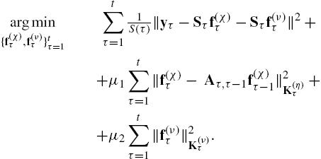
The spatiotemporal model in (8.42), (8.43) can represent multiple forms of spatiotemporal dynamics by judicious selection of the associated parameters. The batch KRR estimator over time yields
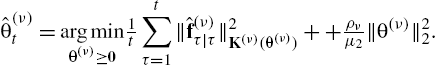
argmin{f(χ)τ,ητ,f(ν)τ,fτ}tτ=1t∑τ=11S(τ)‖yτ−Sτfτ‖2+μ1t∑τ=1‖ητ‖2K(η)τ+μ2t∑τ=1‖f(ν)τ‖2K(ν)τs.t.ητ=f(χ)τ−Aτ,τ−1f(χ)τ−1,fτ=f(ν)τ+f(χ)τ,τ=1,…,t.
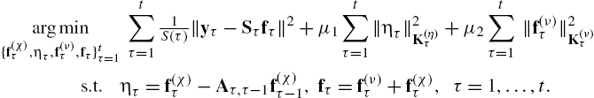
The first term in (8.47) penalizes the fitting error in accordance with (8.1). The scalars ![]() are regularization parameters controlling the effect of the kernel regularizers, while prior information about
are regularization parameters controlling the effect of the kernel regularizers, while prior information about ![]() may guide the selection of the appropriate kernel matrices. The constraints in (8.47) imply adherence to (8.43) and (8.42). Since the
may guide the selection of the appropriate kernel matrices. The constraints in (8.47) imply adherence to (8.43) and (8.42). Since the ![]() are defined over the time evolving
are defined over the time evolving ![]() , a potential approach is to select Laplacian kernels as
, a potential approach is to select Laplacian kernels as ![]() ; see §8.2.2. Next, we rewrite (8.47) in a form amenable to online solvers, namely
; see §8.2.2. Next, we rewrite (8.47) in a form amenable to online solvers, namely
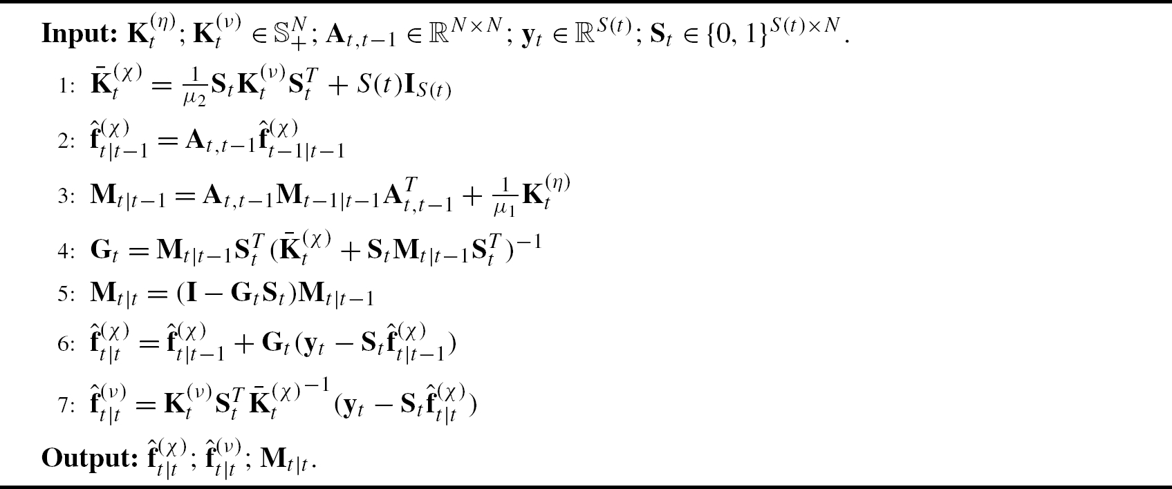
In a batch form the optimization in (8.48) yields ![]() and
and ![]() per slot t with complexity that grows with t. Fortunately, the filtered solutions
per slot t with complexity that grows with t. Fortunately, the filtered solutions ![]() of (8.48) are attained by the kernel kriged Kalman filter (KeKriKF) in an online fashion. For the proof the reader is referred to [58]. One iteration of the proposed KeKriKF is summarized as Algorithm 3. This online estimator—with computational complexity
of (8.48) are attained by the kernel kriged Kalman filter (KeKriKF) in an online fashion. For the proof the reader is referred to [58]. One iteration of the proposed KeKriKF is summarized as Algorithm 3. This online estimator—with computational complexity ![]() per t—tracks the temporal variations of the signal of interest through (8.43) and promotes desired properties such as smoothness over the graph, using
per t—tracks the temporal variations of the signal of interest through (8.43) and promotes desired properties such as smoothness over the graph, using ![]() and
and ![]() . Different from existing KriKF approaches over graphs [55], the KeKriKF takes into account the underlying graph structure in estimating
. Different from existing KriKF approaches over graphs [55], the KeKriKF takes into account the underlying graph structure in estimating ![]() as well as
as well as ![]() . Furthermore, by using
. Furthermore, by using ![]() in (8.16), it can also accommodate dynamic graph topologies. Finally, it should be noted that KeKriKF encompasses as a special case the KriKF, which relies on knowing the statistical properties of the function [55–57,60].
in (8.16), it can also accommodate dynamic graph topologies. Finally, it should be noted that KeKriKF encompasses as a special case the KriKF, which relies on knowing the statistical properties of the function [55–57,60].
Lack of prior information prompts the development of data-driven approaches that efficiently learn the appropriate kernel matrix. Section 8.3.2.3 proposes an online MKL approach for achieving this goal.
8.3.2.3 Online Multikernel Learning
To cope with a lack of prior information about the pertinent kernel, the following dictionaries of kernels will be considered: ![]() and
and ![]() . For the following assume that
. For the following assume that ![]() ,
, ![]() and
and ![]() . Moreover, we postulate that the kernel matrices are of the form
. Moreover, we postulate that the kernel matrices are of the form ![]() and
and ![]() , where
, where ![]() .
.
Next, in accordance with §8.2.3 the coefficients ![]() and
and ![]() can be found by jointly minimizing (8.48) with respect to
can be found by jointly minimizing (8.48) with respect to ![]() and
and ![]() , which yields
, which yields
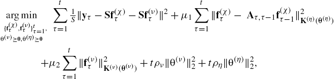
where ![]() are regularization parameters that effect a ball constraint on
are regularization parameters that effect a ball constraint on ![]() and
and ![]() , weighted by t to account for the first three terms that are growing with t. Observe that the optimization problem in (8.49) gives time varying estimates
, weighted by t to account for the first three terms that are growing with t. Observe that the optimization problem in (8.49) gives time varying estimates ![]() and
and ![]() allowing to track the optimal
allowing to track the optimal ![]() and
and ![]() that change over time respectively.
that change over time respectively.
The optimization problem in (8.49) is not jointly convex in ![]() , but it is separately convex in these variables. To solve (8.49) alternating minimization strategies will be employed that suggest optimizing with respect to one variable, while keeping the other variables fixed [61]. If
, but it is separately convex in these variables. To solve (8.49) alternating minimization strategies will be employed that suggest optimizing with respect to one variable, while keeping the other variables fixed [61]. If ![]() are considered fixed, (8.49) reduces to (8.48), which can be solved by Algorithm 3 for the estimates
are considered fixed, (8.49) reduces to (8.48), which can be solved by Algorithm 3 for the estimates ![]() at each t. For
at each t. For ![]() fixed and replaced by
fixed and replaced by ![]() in (8.48) the time varying estimates of
in (8.48) the time varying estimates of ![]() are found by
are found by
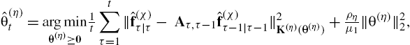
The optimization problems (8.50a) and (8.50b) are strongly convex and iterative algorithms are available based on projected gradient descent (PGD) [62], or the Frank–Wolfe algorithm [63]. When the kernel matrices belong to the Laplacian family (8.16), efficient algorithms that exploit the common eigenspace of the kernels in the dictionary have been developed in [58]. The proposed method reduces the per step computational complexity of PGD from a prohibitive ![]() for general kernels to a more affordable
for general kernels to a more affordable ![]() for Laplacian kernels. The proposed algorithm, termed multikernel KriKF (MKriKF), alternates between computing
for Laplacian kernels. The proposed algorithm, termed multikernel KriKF (MKriKF), alternates between computing ![]() and
and ![]() utilizing the KKriKF and estimating
utilizing the KKriKF and estimating ![]() and
and ![]() from solving (8.50b) and (8.50a).
from solving (8.50b) and (8.50a).
8.3.3 Numerical Tests
This section compares the performance of the methods we discussed in §8.3.1 and §8.3.2 with state-of-the-art alternatives and illustrates some of the trade-offs inherent to time varying function reconstruction through real-data experiments. The source code for the simulations is available at the authors' websites.
Unless otherwise stated, the compared estimators include distributed least squares reconstruction (DLSR) [49] with step size ![]() and parameter
and parameter ![]() ; the least mean squares (LMS) algorithm in [50] with step size
; the least mean squares (LMS) algorithm in [50] with step size ![]() ; the BL instantaneous estimator (BL-IE), which results after applying [11,13,15] separately per t; and the KRR instantaneous estimator (KRR-IE) in (8.36) with a diffusion kernel with parameter σ. DLSR, LMS and BL-IE also use a bandwidth parameter B.
; the BL instantaneous estimator (BL-IE), which results after applying [11,13,15] separately per t; and the KRR instantaneous estimator (KRR-IE) in (8.36) with a diffusion kernel with parameter σ. DLSR, LMS and BL-IE also use a bandwidth parameter B.
Reconstruction via extended graphs. For our first experiment we use a dataset obtained from an epilepsy study [65], which is used to showcase an example analysis of ECoG data (analysis of ECoG data is a standard tool in diagnosing epilepsy). Our next experiment utilizes the ECoG time series in [65] from ![]() electrodes implanted in a patient's brain before and after the onset of a seizure. A symmetric time-invariant adjacency matrix A was obtained using the method in [44] with ECoG data before the onset of the seizure. Function
electrodes implanted in a patient's brain before and after the onset of a seizure. A symmetric time-invariant adjacency matrix A was obtained using the method in [44] with ECoG data before the onset of the seizure. Function ![]() comprises the electrical signal at the nth electrode and tth sampling instant after the onset of the seizure, for a period of
comprises the electrical signal at the nth electrode and tth sampling instant after the onset of the seizure, for a period of ![]() samples. The values of
samples. The values of ![]() were normalized by subtracting the temporal mean of each time series before the onset of the seizure. The goal of the experiment is to illustrate the reconstruction performance of KKF in capturing the complex spatiotemporal dynamics of brain signals.
were normalized by subtracting the temporal mean of each time series before the onset of the seizure. The goal of the experiment is to illustrate the reconstruction performance of KKF in capturing the complex spatiotemporal dynamics of brain signals.
Fig. 8.3A depicts the ![]() , averaged over all sets
, averaged over all sets ![]() , of size
, of size ![]() . For the KKF, a space–time kernel was created (see [51]) with
. For the KKF, a space–time kernel was created (see [51]) with ![]() a time-invariant covariance kernel
a time-invariant covariance kernel ![]() , where
, where ![]() was set to the sample covariance matrix of the time series before the onset of the seizure, with a time-invariant
was set to the sample covariance matrix of the time series before the onset of the seizure, with a time-invariant ![]() . The results clearly show the superior reconstruction performance of the KKF, which successfully exploits the statistics of the signal when available, among competing approaches, even with a small number of samples. This result suggests that the ECoG diagnosis technique could be efficiently conducted even with a smaller number of intracranial electrodes, which may have a positive impact on the patient's experience.
. The results clearly show the superior reconstruction performance of the KKF, which successfully exploits the statistics of the signal when available, among competing approaches, even with a small number of samples. This result suggests that the ECoG diagnosis technique could be efficiently conducted even with a smaller number of intracranial electrodes, which may have a positive impact on the patient's experience.
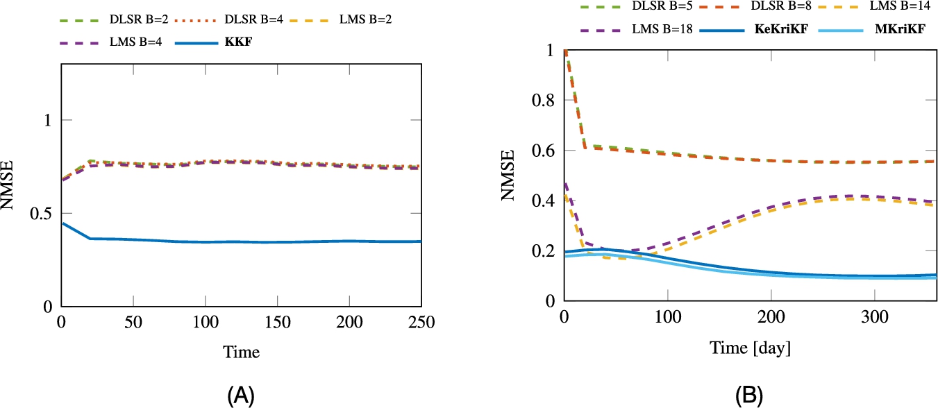
 , βDLSR = 0.5, μLMS = 0.6). (B) NMSE of temperature estimates (μ1 = 1, μ2 = 1, μDLSR = 1.6, βDLSR = 0.5, μLMS = 0.6, α = 10−3, μη = 10−5, rη = 10−6, μν = 2, rν = 0.5, Mν = 40, Mη = 40).
Reconstruction via KeKriKF. The second dataset is provided by the National Climatic Data Center [66] and comprises hourly temperature measurements at ![]() measuring stations across the continental United States in 2010. A time-invariant graph was constructed as in [51], based on geographical distances. The value
measuring stations across the continental United States in 2010. A time-invariant graph was constructed as in [51], based on geographical distances. The value ![]() represents the temperature recorded at the nth station and tth day.
represents the temperature recorded at the nth station and tth day.
Fig. 8.3B reports the performance of different reconstruction algorithms in terms of NMSE, for ![]() . The KeKriKF Algorithm 3 adopts a diffusion kernel for
. The KeKriKF Algorithm 3 adopts a diffusion kernel for ![]() with
with ![]() and for
and for ![]() with
with ![]() . The MKriKF is configured with:
. The MKriKF is configured with: ![]() that contains
that contains ![]() diffusion kernels with parameters
diffusion kernels with parameters ![]() drawn from a Gaussian distribution with mean
drawn from a Gaussian distribution with mean ![]() and variance
and variance ![]() ;
; ![]() that contains
that contains ![]()
![]() with parameters
with parameters ![]() drawn from a Gaussian distribution with mean
drawn from a Gaussian distribution with mean ![]() and variance
and variance ![]() . The specific kernel selection for KeKriKF leads to the smallest NMSE error and was selected using cross validation. Observe that MKriKF captures the spatiotemporal dynamics, successfully explores the pool of available kernels and achieves superior performance.
. The specific kernel selection for KeKriKF leads to the smallest NMSE error and was selected using cross validation. Observe that MKriKF captures the spatiotemporal dynamics, successfully explores the pool of available kernels and achieves superior performance.
The third dataset is provided by the World Bank Group [67] and is comprised of the gross domestic product (GDP) per capita values for ![]() countries for the years 1960–2016. A time-invariant graph was constructed using the correlation between the GDP values for the first 25 years of different countries. The graph function
countries for the years 1960–2016. A time-invariant graph was constructed using the correlation between the GDP values for the first 25 years of different countries. The graph function ![]() denotes the GDP value reported for the nth country and tth year for
denotes the GDP value reported for the nth country and tth year for ![]() . The graph Fourier transform of the GDP values shows that the graph frequencies
. The graph Fourier transform of the GDP values shows that the graph frequencies ![]() ,
, ![]() , take small values and large values otherwise. Motivated by the aforementioned observation, the KKriKF is configured with a band-reject kernel
, take small values and large values otherwise. Motivated by the aforementioned observation, the KKriKF is configured with a band-reject kernel ![]() that results after applying
that results after applying ![]() for
for ![]() and
and ![]() otherwise in (8.16) with
otherwise in (8.16) with ![]() and for
and for ![]() with
with ![]() . The MKriKF adopts a
. The MKriKF adopts a ![]() that contains band-reject kernels with
that contains band-reject kernels with ![]() ,
, ![]() ,
, ![]() that result in
that result in ![]() kernels and a
kernels and a ![]() that contains
that contains ![]() with
with ![]() drawn from a Gaussian distribution with mean
drawn from a Gaussian distribution with mean ![]() and variance
and variance ![]() . Next, the performance of different algorithms in tracking the GDP value is evaluated after sampling
. Next, the performance of different algorithms in tracking the GDP value is evaluated after sampling ![]() countries.
countries.
Fig. 8.4 illustrates the actual GDP as well as GDP estimates for Greece, which is not contained in the sampled countries. Clearly, MKriKF, which learns the pertinent kernels from the data, achieves roughly the same performance as KKriKF, which is configured manually to obtain the smallest possible NMSE.
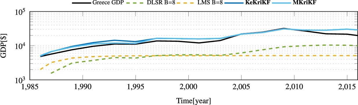
8.3.4 Summary
The task of reconstructing functions defined on graphs arises naturally in a plethora of applications. The kernel-based approach offers a clear, principled and intuitive way for tackling this problem. In this chapter, we gave a contemporary treatment of this framework focusing on both time-invariant and time evolving domains. The methods presented herein offer the potential of providing an expressive way to tackle interesting real-world problems. Besides illustrating the effectiveness of the discussed approaches, our tests were also chosen to showcase interesting application areas as well as reasonable modeling approaches for the interested readers to build upon. For further details about the models discussed here and their theoretical properties, the reader is referred to [23,39,59,58,68,69] and the references therein.