
Adaptive H∞ Tracking Control of Nonlinear Systems Using Reinforcement Learning
Hamidreza Modares⁎; Bahare Kiumarsi†; Kyriakos G. Vamvoudakis‡; Frank L. Lewis†,§ ⁎Missouri University of Science and Technology, Rolla, MO, United States
†UTA Research Institute, University of Texas at Arlington, Fort Worth, TX, United States
‡Virginia Tech, Blacksburg, VA, United States
§State Key Laboratory of Synthetical Automation for Process Industries, Northeastern University, Shenyang, China
Abstract
This chapter presents online solutions to the optimal H∞![]() tracking of nonlinear systems to attenuate the effect of disturbance on the performance of the systems. To obviate the requirement of the complete knowledge of the system dynamics, reinforcement learning (RL) is used to learn the solutions to the Hamilton–Jacobi–Isaacs equations arising from solving the H∞
tracking of nonlinear systems to attenuate the effect of disturbance on the performance of the systems. To obviate the requirement of the complete knowledge of the system dynamics, reinforcement learning (RL) is used to learn the solutions to the Hamilton–Jacobi–Isaacs equations arising from solving the H∞![]() tracking problem. Off-policy RL algorithms are designed for continuous-time systems, which allows the reuse of data for learning and consequently leads to data efficient RL algorithms. A solution is first presented for the H∞
tracking problem. Off-policy RL algorithms are designed for continuous-time systems, which allows the reuse of data for learning and consequently leads to data efficient RL algorithms. A solution is first presented for the H∞![]() optimal tracking control of affine nonlinear systems. It is then extended to a special class of nonlinear nonaffine systems. It is shown that for the nonaffine systems existence of a stabilizing solution depends on the performance function. A performance function is designed to assure the existence of the solution to a class of nonaffine system, while taking into account the input constraints.
optimal tracking control of affine nonlinear systems. It is then extended to a special class of nonlinear nonaffine systems. It is shown that for the nonaffine systems existence of a stabilizing solution depends on the performance function. A performance function is designed to assure the existence of the solution to a class of nonaffine system, while taking into account the input constraints.
Keywords
H∞![]() control; Optimal tracking; Reinforcement learning
control; Optimal tracking; Reinforcement learning
Chapter Points
- • The result of this approach is to design an online data-based solution to the H∞ tracking control problem.
- • Reinforcement learning is employed to learn the solution to the H∞ tracking in real-time and without requiring the system dynamics.
14.1 Introduction
Reinforcement learning (RL) [1–3], inspired by learning mechanisms observed in animals, is concerned with how an agent or decision maker takes actions so as to optimize a cost of its long-term interactions with the environment. The cost function is prescribed and captures some desired system behaviors such as minimizing the transient error and minimizing the control effort for achieving a specific goal. The agent learns an optimal policy so that, by taking actions produced based on this policy, the long-term cost function is optimized. Similar to RL, optimal control involves finding an optimal policy by optimizing a long-term performance criterion. Strong connections between RL and optimal control have prompted a major effort towards introducing and developing online and model-free RL algorithms to learn the solution to optimal control problems [4–6].
RL methods have been successfully used to solve the optimal regulation problems by learning the solution to the so-called Hamilton–Jacobi equations arising from both optimal H2![]() [7–18] and H∞
[7–18] and H∞![]() [19–30] regulation problems. For continuous-time (CT) systems, [8,9] proposed a promising RL algorithm, called integral RL (IRL), to learn the solution to the Hamilton–Jacobi–Bellman (HJB) equations using only partial knowledge about the system dynamics. They used an iterative online policy iteration [31] procedure to implement their IRL algorithm. The original IRL algorithm and many of its extensions are on-policy algorithms. That is, the policy that is applied to the system to generate data for learning (behavior policy) is the same as the policy that is being updated and learned about (target policy). The work [15] presented an off-policy RL algorithms for CT systems in which the behavior policy could be different from the target policy. This algorithm does not require any knowledge of the system dynamics and is data efficient because it reuses the data generated by the behavior policy to learn as many target policies as required. Many variants and extensions of off-policy RL algorithms are presented in the literature. Other than the IRL-based PI algorithms and off-policy RL algorithms, efficient synchronous PI algorithms with guaranteed closed-loop stability were proposed for CT systems in [7,11,12] to learn the solution to the HJB equation. Synchronous IRL algorithms were also presented for solving the HJB equation in [23,32].
[19–30] regulation problems. For continuous-time (CT) systems, [8,9] proposed a promising RL algorithm, called integral RL (IRL), to learn the solution to the Hamilton–Jacobi–Bellman (HJB) equations using only partial knowledge about the system dynamics. They used an iterative online policy iteration [31] procedure to implement their IRL algorithm. The original IRL algorithm and many of its extensions are on-policy algorithms. That is, the policy that is applied to the system to generate data for learning (behavior policy) is the same as the policy that is being updated and learned about (target policy). The work [15] presented an off-policy RL algorithms for CT systems in which the behavior policy could be different from the target policy. This algorithm does not require any knowledge of the system dynamics and is data efficient because it reuses the data generated by the behavior policy to learn as many target policies as required. Many variants and extensions of off-policy RL algorithms are presented in the literature. Other than the IRL-based PI algorithms and off-policy RL algorithms, efficient synchronous PI algorithms with guaranteed closed-loop stability were proposed for CT systems in [7,11,12] to learn the solution to the HJB equation. Synchronous IRL algorithms were also presented for solving the HJB equation in [23,32].
Although RL algorithms have been widely used to solve the optimal regulation problems, few results considered solving the optimal tracking control problem (OTCP) for both discrete-time [33–36] and continuous-time systems [6,37]. Moreover, existing methods for continuous-time systems require the exact knowledge of the system dynamics a priori while finding the feedforward part of the control input using either the dynamic inversion concept or the solution of output regulator equations [39–41]. While the importance of the RL algorithms is well understood for solving optimal regulation problems for uncertain systems, the requirement of the exact knowledge of the system dynamics for finding the steady-state part of the control input in the existing OTCP formulation does not allow for direct extending of the IRL algorithm for solving the OTCP.
In this chapter, we develop adaptive optimal controllers based on the RL techniques to learn the optimal H∞![]() tracking control solutions for nonlinear continuous-time systems without knowing the system dynamics or the command generator dynamics. An augmented system is first constructed from the tracking error dynamics and the command generator dynamics to introduce a new discounted performance function for the OTCP. The tracking Hamilton–Jacobi–Isaac (HJI) equations are then derived to solve OTCPs. Off-policy RL algorithms, implemented on an actor-critic structure, are used to find the solution to the tracking HJI equations online using only measured data along the augmented system trajectories. These algorithms are developed for both affine and nonaffine nonlinear systems. Therefore, they can be employed in control of many real-world applications, including robot manipulators, mobile robots, unmanned aerial vehicles (UAVs), power systems and human–robot interaction systems.
tracking control solutions for nonlinear continuous-time systems without knowing the system dynamics or the command generator dynamics. An augmented system is first constructed from the tracking error dynamics and the command generator dynamics to introduce a new discounted performance function for the OTCP. The tracking Hamilton–Jacobi–Isaac (HJI) equations are then derived to solve OTCPs. Off-policy RL algorithms, implemented on an actor-critic structure, are used to find the solution to the tracking HJI equations online using only measured data along the augmented system trajectories. These algorithms are developed for both affine and nonaffine nonlinear systems. Therefore, they can be employed in control of many real-world applications, including robot manipulators, mobile robots, unmanned aerial vehicles (UAVs), power systems and human–robot interaction systems.
14.2 H∞ Optimal Tracking Control for Nonlinear Affine Systems
Existing solutions to the H∞![]() tracking problem are composed of two steps [38–41]. A feedforward control input is designed to guarantee perfect tracking using either dynamic inversion or by solving the so-called output regulator equations in the first step. A feedback control input is designed in the second step by solving an HJI equation to stabilize the tracking error dynamics. In these methods, procedures for computing the feedback and feedforward terms are based on offline solution methods which require complete knowledge of the system dynamics. In this section, a new formulation for the H∞
tracking problem are composed of two steps [38–41]. A feedforward control input is designed to guarantee perfect tracking using either dynamic inversion or by solving the so-called output regulator equations in the first step. A feedback control input is designed in the second step by solving an HJI equation to stabilize the tracking error dynamics. In these methods, procedures for computing the feedback and feedforward terms are based on offline solution methods which require complete knowledge of the system dynamics. In this section, a new formulation for the H∞![]() tracking is presented which allows developing model-free RL solutions.
tracking is presented which allows developing model-free RL solutions.
Consider the nonlinear time-invariant system given as
˙x(t)=f(x(t))+g(x(t))u(t)+k(x(t))w(t),
where x(t)∈Rn![]() , u(t)∈Rm
, u(t)∈Rm![]() and w(t)∈Rp
and w(t)∈Rp![]() represent the state of the system, the control input and the external disturbance of the system, respectively. The drift dynamics is represented by f(x(t))∈Rn
represent the state of the system, the control input and the external disturbance of the system, respectively. The drift dynamics is represented by f(x(t))∈Rn![]() , g(x(t))∈Rn×m
, g(x(t))∈Rn×m![]() is the input dynamics and k(x(t))∈Rp
is the input dynamics and k(x(t))∈Rp![]() is the disturbance dynamics. It is assumed that f(0)=0
is the disturbance dynamics. It is assumed that f(0)=0![]() and f(x(t))
and f(x(t))![]() , g(x(t)
, g(x(t)![]() and k(x(t))
and k(x(t))![]() are unknown Lipschitz functions and the system is stabilizable.
are unknown Lipschitz functions and the system is stabilizable.
Assumption 1
Let r(t)![]() be the bounded reference trajectory and assume that there exists a Lipschitz continuous command generator function hd(t)∈Rn
be the bounded reference trajectory and assume that there exists a Lipschitz continuous command generator function hd(t)∈Rn![]() with hd(0)=0
with hd(0)=0![]() such that
such that
˙r(t)=hd(t)r(t).
Define the tracking error
ed(t)≜x(t)−r(t).
Using (14.1)–(14.3), the tracking error dynamics is given by
˙ed(t)=f(x(t))+g(x(t))u(t)+k(x(t))w(t)−hd(r(t)).
The performance output to be controlled is defined such that it satisfies
‖z(t)‖2=edTQed+uTRu.
The goal of the H∞![]() tracking is to attenuate the effect of the disturbance input w on the performance output z. Before defining the H∞
tracking is to attenuate the effect of the disturbance input w on the performance output z. Before defining the H∞![]() tracking control problem, we define the following general L2
tracking control problem, we define the following general L2![]() -gain or disturbance attenuation condition.
-gain or disturbance attenuation condition.
Definition 1
Bounded L2![]() -gain or disturbance attenuation
-gain or disturbance attenuation
The nonlinear system (14.1) is said to have L2![]() -gain less than or equal to γ if the following disturbance attenuation condition is satisfied for all w∈L2[0,∞)
-gain less than or equal to γ if the following disturbance attenuation condition is satisfied for all w∈L2[0,∞)![]() :
:
∫∞te−α(τ−t)‖z(τ)‖2dτ∫∞te−α(τ−t)‖w(τ)‖2dτ⩽γ2,
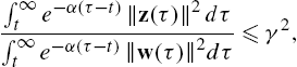
where α>0![]() is the discount factor and γ represents the amount of attenuation from the disturbance input w(t)
is the discount factor and γ represents the amount of attenuation from the disturbance input w(t)![]() to the defined performance output variable z(t)
to the defined performance output variable z(t)![]() .
.
The disturbance attenuation condition (14.6) implies that the effect of the disturbance input to the desired performance output is attenuated by a degree at least equal to γ. The desired performance output represents a meaningful cost in the sense that it includes a positive penalty on the tracking error and a positive penalty on the control effort. The use of the discount factor is essential. This is because the feedforward part of the control input does not converge to zero in general and thus penalizing the control input in the performance function without a discount factor makes the performance function unbounded.
Using (14.5) in (14.6) one has
∫∞te−α(τ−t)(edTQed+uTRu)dτ⩽γ2∫∞te−α(τ−t)(wTw)dτ.

Definition 2
H∞![]() optimal tracking
optimal tracking
The H∞![]() tracking control problem is to find a control policy u=β(ed,r)
tracking control problem is to find a control policy u=β(ed,r)![]() for some smooth function β depending on the tracking error e and the reference trajectory r, such that:
for some smooth function β depending on the tracking error e and the reference trajectory r, such that:
(i) The closed-loop system ˙x=f(x)+g(x)β(ed,r)+k(x)w![]() satisfies the attenuation condition (14.7).
satisfies the attenuation condition (14.7).
(ii) The tracking error dynamics (14.4) with w=0![]() is locally asymptotically stable.
is locally asymptotically stable.
The main difference between Definition 2 and the standard definition of the H∞![]() tracking control problem (see [38], Definition 5.2.1) is that a more general disturbance attenuation condition is defined here. Previous work on the H∞
tracking control problem (see [38], Definition 5.2.1) is that a more general disturbance attenuation condition is defined here. Previous work on the H∞![]() optimal tracking divides the control input into feedback and feedforward parts. The feedforward part is first obtained separately without considering any optimality criterion. Then, the problem of optimal design of the feedback part is reduced to an H∞
optimal tracking divides the control input into feedback and feedforward parts. The feedforward part is first obtained separately without considering any optimality criterion. Then, the problem of optimal design of the feedback part is reduced to an H∞![]() optimal regulation problem. In contrast, in the new formulation, both feedback and feedforward parts of the control input are obtained simultaneously and optimally as a result of the defined L2
optimal regulation problem. In contrast, in the new formulation, both feedback and feedforward parts of the control input are obtained simultaneously and optimally as a result of the defined L2![]() -gain with discount factor in (14.7).
-gain with discount factor in (14.7).
14.2.1 HJI Equation for H∞ Optimal Tracking
In this section, it is first shown that the problem of solving the H∞![]() tracking problem can be transformed into a min–max optimization problem subject to an augmented system composed of the tracking error dynamics and the command generator dynamics. A tracking HJI equation is then developed which gives the solution to the min–max optimization problem. The stability and L2
tracking problem can be transformed into a min–max optimization problem subject to an augmented system composed of the tracking error dynamics and the command generator dynamics. A tracking HJI equation is then developed which gives the solution to the min–max optimization problem. The stability and L2![]() -gain boundedness of the tracking HJI control solution are discussed.
-gain boundedness of the tracking HJI control solution are discussed.
Define the augmented system state
X(t)=[ed(t)Tr(t)T]T∈R2n,
where ed(t)![]() is the tracking error defined in (14.3) and r(t)
is the tracking error defined in (14.3) and r(t)![]() is the reference trajectory.
is the reference trajectory.
Using (14.2) and (14.4), define the augmented system
˙X(t)=F(X(t))+G(X(t))u(t)+K(X(t))w(t),
where u(t)=u(X(t))![]() and
and
F(X)=[f(ed+r)−hd(r)hd(r)],G(X)=[g(ed+r)0],K(X)=[k(ed+r)0].

The disturbance attenuation condition (14.7) using the augmented state becomes
∫∞te−α(τ−t)(XTQTX+uTRu)dτ⩽γ2∫∞te−α(τ−t)(wTw)dτ,

where
QT=[Q000].

Based on (14.9), define the performance function
J(u,w)=∫∞te−α(τ−t)(XTQTX+uTRu−γ2wTw)dτ.

Solvability of the H∞![]() control problem is equivalent to solvability of the following zero-sum game [42]:
control problem is equivalent to solvability of the following zero-sum game [42]:
V⋆(X(t))=J(u⋆,w⋆)=minumaxdJ(u,w),
where J is defined in (14.10) and V⋆(X(t))![]() is defined as the optimal value function. This two-player zero-sum game control problem has a unique solution if a game theoretic saddle point exists, i.e., if the following Nash condition holds:
is defined as the optimal value function. This two-player zero-sum game control problem has a unique solution if a game theoretic saddle point exists, i.e., if the following Nash condition holds:
V⋆(X(t))=minumaxdJ(u,w)=maxdminuJ(u,w).
Differentiating (14.10), note that V(X(t))=J(u(t),w(t))![]() gives the following Bellman equation:
gives the following Bellman equation:
H(V,u,w)Δ=XTQTX+uTRu−γ2wTw−αV+VXT(F+G u+K w)=0,
where F≜F(X)![]() , G≜G(X)
, G≜G(X)![]() , K≜K(X)
, K≜K(X)![]() and VX=∂V/∂X
and VX=∂V/∂X![]() .
.
Applying stationarity conditions ∂H(V⋆,u,w)/∂u=0,∂H(V⋆,u,w)/∂w=0![]() [43] gives the optimal control and disturbance inputs as
[43] gives the optimal control and disturbance inputs as
u⋆=−12R−1GTVX⋆,
w⋆=12γ2KTVX⋆,
where V⋆![]() is the optimal value function defined in (14.11). Substituting the control input (14.13) and the disturbance (14.14) into (14.12), the following tracking HJI equation is obtained:
is the optimal value function defined in (14.11). Substituting the control input (14.13) and the disturbance (14.14) into (14.12), the following tracking HJI equation is obtained:
H(V⋆,u⋆,w⋆)≜XTQTX+VX⋆TF−αVX−14VX⋆TGTR−1GVX⋆+14γ2VX⋆TK KTVX⋆=0.

It is shown in [44] that the control solution (14.13)–(14.15) satisfies the disturbance attenuation condition (14.9) (part (i) of Definition 2) and that it guarantees the stability of the tracking error dynamics (14.4) without the disturbance (part (ii) of Definition 2), if the discount factor is less than an upper bound.
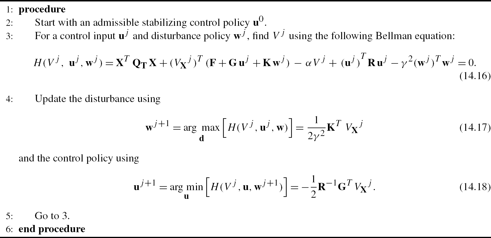
14.2.2 Off-Policy IRL for Learning the Tracking HJI Equation
In this section, an off-policy RL algorithm is first given to learn this control solution online and without requiring any knowledge of the system dynamics.
The Bellman equation (14.12) is linear in the cost function V, while the HJI equation (14.15) is nonlinear in the value function V⋆![]() . Therefore, solving the Bellman equation for V is easier than solving the HJI for V⋆
. Therefore, solving the Bellman equation for V is easier than solving the HJI for V⋆![]() . Instead of directly solving for V⋆
. Instead of directly solving for V⋆![]() , a policy iteration (PI) algorithm iterates on both control and disturbance players to break the HJI equation into a sequence of differential equations linear in the cost. An offline PI algorithm for solving the H∞
, a policy iteration (PI) algorithm iterates on both control and disturbance players to break the HJI equation into a sequence of differential equations linear in the cost. An offline PI algorithm for solving the H∞![]() optimal tracking problem is given as follows.
optimal tracking problem is given as follows.
Algorithm 1 extends the results of the simultaneous RL algorithm in [27] to the tracking problem. The convergence of this algorithm to the minimal nonnegative solution of the HJI equation was shown in [27]. In fact, similar to [27], the convergence of Algorithm 1 can be established by proving that iteration on (14.16) is essentially a Newton iterative sequence which converges to the unique solution of the HJI equation (14.15).
Algorithm 1 requires complete knowledge of the system dynamics. In the following, the off-policy IRL algorithm, which was presented in [14,15] for solving the H2![]() optimal regulation problem, is extended here to solve the H∞
optimal regulation problem, is extended here to solve the H∞![]() optimal tracking for systems with completely unknown dynamics. To this end, the system dynamics (14.8) is first written as
optimal tracking for systems with completely unknown dynamics. To this end, the system dynamics (14.8) is first written as
˙X=F+Guj+Kwj+G(u−uj)+K(w−wj),
where uj∈Rm![]() and wj∈Rq
and wj∈Rq![]() are policies to be updated. In this equation, the control input u is the behavior policy which is applied to the system to generate data for learning, while uj
are policies to be updated. In this equation, the control input u is the behavior policy which is applied to the system to generate data for learning, while uj![]() is the target policy which is evaluated and updated using data generated by the behavior policy. The fixed control policy u should be a stable and exploring control policy. Moreover, the disturbance input w is the actual external disturbance that comes from an external source and is not under our control. However, the disturbance wj
is the target policy which is evaluated and updated using data generated by the behavior policy. The fixed control policy u should be a stable and exploring control policy. Moreover, the disturbance input w is the actual external disturbance that comes from an external source and is not under our control. However, the disturbance wj![]() is the disturbance that is evaluated and updated. One advantage of this off-policy IRL Bellman equation is that, in contrast to on-policy RL-based methods, the disturbance input that is applied to the system does not require to be adjustable.
is the disturbance that is evaluated and updated. One advantage of this off-policy IRL Bellman equation is that, in contrast to on-policy RL-based methods, the disturbance input that is applied to the system does not require to be adjustable.
Differentiating Vj(X)![]() along with the system dynamics (14.19) and using (14.16)–(14.18) gives
along with the system dynamics (14.19) and using (14.16)–(14.18) gives
˙Vj=(VXj)T(F+Guj+Kwj)+(VXj)TG(u−uj)+(VXj)TK(w−wj)=αVj−XTQTX−(uj)TRuj+γ2(wj)Twj−2(uj+1)TR(u−uj)+2γ2(wj+1)T(w−wj).

Multiplying both sides of (14.20) by e−α(τ−t)![]() and integrating from both sides yields the following off-policy IRL Bellman equation:
and integrating from both sides yields the following off-policy IRL Bellman equation:
e−αTVj(X(t+T))−Vj(X(t))=∫t+Tte−α(τ−t)(−XTQTX−(uj)TRuj+γ2(wj)Twj)dτ+∫t+Tte−α(τ−t)(−2(uj+1)TR(u−uj)+2γ2(wj+1)T(w−wj))dτ.

Note that, for a fixed control policy u (the policy that is applied to the system) and a given disturbance w (the actual disturbance that is applied to the system), Eq. (14.21) can be solved for both the value function Vj![]() and the updated policies uj+1
and the updated policies uj+1![]() and wj+1
and wj+1![]() simultaneously.
simultaneously.
The following algorithm uses the off-policy tracking Bellman equation (14.21) to iteratively solve the HJI equation (14.15) without requiring any knowledge of the system dynamics. The implementation of this algorithm is discussed in the next subsection. It is shown how the data collected from a fixed control policy u are reused to evaluate many updated control policies ui![]() sequentially until convergence to the optimal solution is achieved.
sequentially until convergence to the optimal solution is achieved.
Inspired by the off-policy algorithm in [14], Algorithm 2 has two separate phases. First, a fixed initial exploratory control policy u is applied and the system information is recorded over the time interval T. Second, without requiring any knowledge of the system dynamics, the information collected in phase 1 is repeatedly used to find a sequence of updated policies uj![]() and wj
and wj![]() converging to u⋆
converging to u⋆![]() and w⋆
and w⋆![]() . Note that Eq. (14.23) is a scalar equation and can be solved in a least square sense after collecting enough data samples from the system. It is shown in the following section how to collect required information in phase 1 and reuse it in phase 2 in a least square sense to solve (14.23) for Vj
. Note that Eq. (14.23) is a scalar equation and can be solved in a least square sense after collecting enough data samples from the system. It is shown in the following section how to collect required information in phase 1 and reuse it in phase 2 in a least square sense to solve (14.23) for Vj![]() , uj+1
, uj+1![]() and wj+1
and wj+1![]() simultaneously. After the learning is done and the optimal control policy u⋆
simultaneously. After the learning is done and the optimal control policy u⋆![]() is found, it can be applied to the system.
is found, it can be applied to the system.

14.2.3 Implementing Algorithm 2 Using Neural Networks
In order to implement the off-policy RL Algorithm 2, it is required to reuse the collected information found by applying a fixed control policy u to the system to solve Eq. (14.23) for Vj![]() , uj+1
, uj+1![]() and wj+1
and wj+1![]() iteratively. Three neural networks (NNs), i.e., the actor NN, the critic NN and the disturber NN, are used here to approximate the value function and the updated control and disturbance policies in the Bellman equation (14.23). That is, the solution Vj
iteratively. Three neural networks (NNs), i.e., the actor NN, the critic NN and the disturber NN, are used here to approximate the value function and the updated control and disturbance policies in the Bellman equation (14.23). That is, the solution Vj![]() , uj+1
, uj+1![]() and wj+1
and wj+1![]() of the Bellman equation (14.23) is approximated by three NNs as
of the Bellman equation (14.23) is approximated by three NNs as
ˆVj(X)=ˆW1Tσ(X),
ˆuj+1(X)=ˆW2Tϕ(X),
ˆwj+1(X)=ˆW3Tφ(X),
where σ=[σ1,...,σl1]∈Rl1![]() , ϕ=[ϕ1,...,ϕl2]∈Rl2
, ϕ=[ϕ1,...,ϕl2]∈Rl2![]() and φ=[φ1,...,φl3]∈Rl3
and φ=[φ1,...,φl3]∈Rl3![]() provide suitable basis function vectors, ˆW1∈Rl1
provide suitable basis function vectors, ˆW1∈Rl1![]() , ˆW2∈Rm×l2
, ˆW2∈Rm×l2![]() and ˆW3∈Rq×l3
and ˆW3∈Rq×l3![]() are constant weight vectors and l1
are constant weight vectors and l1![]() , l2
, l2![]() and l3
and l3![]() are the number of neurons. Define v1=[v11,...,vm1]T=u−uj
are the number of neurons. Define v1=[v11,...,vm1]T=u−uj![]() , v2=[v21,...,v2q]T=w−wj
, v2=[v21,...,v2q]T=w−wj![]() and assume R=diag(r,...,rm)
and assume R=diag(r,...,rm)![]() . Then, substituting (14.24)–(14.26) in (14.23) yields
. Then, substituting (14.24)–(14.26) in (14.23) yields
e(t)=ˆW1T(e−αTσ(X(t+T))−σ(X(t)))−∫t+Tte−α(τ−t)(−XTQTX−(uj)TRuj+γ2(wj)Twj)dτ+2m∑l=1rl∫t+Tte−α(τ−t)ˆW2,lTϕ(X(t))v1ldτ−2γ2q∑k=1∫t+Tte−α(τ−t)ˆW3,kTφ(X(t))v2kdτ,
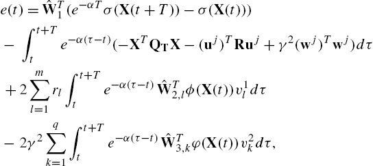
where e(t)![]() is the Bellman approximation error, ˆW2,l
is the Bellman approximation error, ˆW2,l![]() is the lth column of ˆW2
is the lth column of ˆW2![]() and ˆW3,k
and ˆW3,k![]() is the kth column of ˆW3
is the kth column of ˆW3![]() . The Bellman approximation error is the continuous-time counterpart of the temporal difference (TD) [10]. In order to bring the TD error to its minimum value, the least squares method is used. To this end, rewrite Eq. (14.27) as
. The Bellman approximation error is the continuous-time counterpart of the temporal difference (TD) [10]. In order to bring the TD error to its minimum value, the least squares method is used. To this end, rewrite Eq. (14.27) as
y(t)+e(t)=ˆWTh(t),
where
ˆW=[ˆW1T,ˆW2,lT,...,ˆW2,mT,ˆW3,1T,...,ˆW3,qT]T∈Rl1+m×l2+q×l3,h(t)=[e−αTσ(X(t+T))−σ(X(t)))2r1∫t+Tte−α(τ−t)ϕ(X(t))v11dτ⋮2rm∫t+Tte−α(τ−t)ϕ(X(t))v1mdτ−2γ2∫t+Tte−α(τ−t)φ(X(t))v21dτ⋮−2γ2∫t+Tte−α(τ−t)φ(X(t))v2qdτ],

y(t)=∫t+Tte−α(τ−t)(−XTQTX−(uj)TRuj+γ2(wj)Twj)dτ.

The parameter vector ˆW![]() , which gives the approximated value function, actor and disturbance (14.24)–(14.26), is found by minimizing, in the least squares sense, the Bellman error. Assume that the systems state, input and disturbance information are collected at N⩾l1+m×l2+q×l3
, which gives the approximated value function, actor and disturbance (14.24)–(14.26), is found by minimizing, in the least squares sense, the Bellman error. Assume that the systems state, input and disturbance information are collected at N⩾l1+m×l2+q×l3![]() (the number of independent elements in ˆW
(the number of independent elements in ˆW![]() ) points t1
) points t1![]() to tN
to tN![]() in the state space, over the same time interval T in phase 1. Then, for a given uj
in the state space, over the same time interval T in phase 1. Then, for a given uj![]() and wj
and wj![]() , one can use this information to evaluate (14.29) and (14.30) at N points to form
, one can use this information to evaluate (14.29) and (14.30) at N points to form
H=[h(t1),....,h(tN)],Y=[y(t1),....,y(tN)]T.
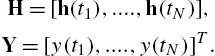
The least squares solution to (14.28) is then equal to
ˆW=(HHT)−1HY,
which gives Vj![]() , uj+1
, uj+1![]() and wj+1
and wj+1![]() . Note that although X(t+T)
. Note that although X(t+T)![]() appears in Eq. (14.27), this equation is solved in a least square sense after observing N samples X(t)
appears in Eq. (14.27), this equation is solved in a least square sense after observing N samples X(t)![]() , X(t+T)
, X(t+T)![]() , …, X(t+NT)
, …, X(t+NT)![]() . Therefore, the knowledge of the system is not required to predict the future state X(t+T)
. Therefore, the knowledge of the system is not required to predict the future state X(t+T)![]() at time t to solve (14.27).
at time t to solve (14.27).
14.3 H∞ Optimal Tracking Control for a Class of Nonlinear Nonaffine Systems
This section considers the design of an RL-based optimal tracking control solution for a class of nonaffine systems.
14.3.1 A Class of Nonaffine Dynamical Systems
A special class of nonaffine systems can be described as
˙X(t)=f(X(t))+g(X(t))L(u)+Dw(t),
where X(t)∈Rn![]() , u(t)∈Rm
, u(t)∈Rm![]() and w(t)∈Rp
and w(t)∈Rp![]() are the state of the system, the control input and the external disturbance input, respectively. The functions f(X(t))
are the state of the system, the control input and the external disturbance input, respectively. The functions f(X(t))![]() and g(X(t))
and g(X(t))![]() are Lipschitz functions. This system is affine in a nonlinear function L(.)
are Lipschitz functions. This system is affine in a nonlinear function L(.)![]() of the control input u(t)
of the control input u(t)![]() . This class of nonaffine systems allows the definition of a new performance function for the optimal H∞
. This class of nonaffine systems allows the definition of a new performance function for the optimal H∞![]() problem such that the existence of the constrained optimal control is assured (if any exists).
problem such that the existence of the constrained optimal control is assured (if any exists).
The following example shows that the UAV as a real-world application can be presented in the form of (14.31).
Example 1
A general class of nonlinear nonaffine UAV systems has the following well-known form:
˙x1=Vcosγcosψ+d1w1,˙x2=Vcosγsinψ+d2w2,˙x3=−Vsinγ+d3w3,˙V=−α2V2−gsinγ+α1ˉT−α3nz−α4n2zV2,˙γ=gV(nzcosϕ−cosγ),˙ψ=gVcosγnzsinϕ,

with
nx=ˉTˉTmaxcosα−Dmg,nx=ˉTˉTmaxsinα+Kmg,

where x1![]() , x2
, x2![]() , x3
, x3![]() are the UAV location coordinates, γ is the pitch angle, ψ is the heading angle, ϕ is bank angle, V is the UAV velocity and m is the mass of the UAV. The terms nx
are the UAV location coordinates, γ is the pitch angle, ψ is the heading angle, ϕ is bank angle, V is the UAV velocity and m is the mass of the UAV. The terms nx![]() and nz
and nz![]() denote longitudinal and normal components of the load factor, depending on the current thrust ˉT
denote longitudinal and normal components of the load factor, depending on the current thrust ˉT![]() , drag force D and lift force K (g is the acceleration due to gravity) [45].
, drag force D and lift force K (g is the acceleration due to gravity) [45].
Define the state of the UAV as
X={x1,x2,x3,V,γ,ψ}T
and the control input and disturbance inputs (wind velocity) as u(t)=[ˉT,nz,ϕ]T=[u1u2u3]T![]() and w(t)
and w(t)![]() , respectively. The constraints on the control input are as follows:
, respectively. The constraints on the control input are as follows:
|u1|⩽ˉu1,|u2|⩽ˉu2.

Using (14.32) and (14.33), the UAV dynamics can be written as a nonlinear nonaffine CT system as
˙X(t)=M(X(t),u(t))+Dw(t),
with
D=[d1d2d3000]T,M(X,u)=[x4cos(x5)cos(x6)x4cos(x5)sin(x6)−x4sin(x5)−α2x24−gsin(x5)+α1u1−α3u2−α4u22x24gx4(−cos(x5)+u2cos(u3))gx4cos(x5)u2sin(u3)].

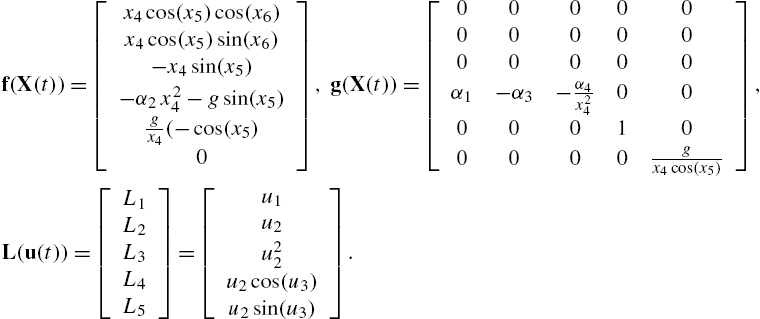
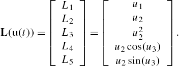
The UAV dynamics (14.35) can be written in the form of (14.31) with
f(X(t))=[x4cos(x5)cos(x6)x4cos(x5)sin(x6)−x4sin(x5)−α2x24−gsin(x5)gx4(−cos(x5)0],g(X(t))=[000000000000000α1−α3−α4x2400000100000gx4cos(x5)],L(u(t))=[L1L2L3L4L5]=[u1u2u22u2cos(u3)u2sin(u3)].
Eq. (14.31) represents a large class of nonaffine systems far larger than the systems that are affine in the control itself. In fact, most aircraft dynamics can be expressed in the form of (14.31) if the lift equation satisfies certain assumptions [45].
14.3.2 Performance Function and H∞ Control Tracking for Nonaffine Systems
It is shown in [46] that the existence of an admissible optimal control solution for nonaffine systems depends on how the utility function r(X,u)![]() is defined. Moreover, to deal with the input constraints, a nonquadratic performance index needs to be defined as follows.
is defined. Moreover, to deal with the input constraints, a nonquadratic performance index needs to be defined as follows.
Let the reference trajectory be generated by the command generator dynamics (14.2). The performance or control output z(t)![]() is defined such that it satisfies
is defined such that it satisfies
‖z(t)‖2=(X−r)TQ(X−r)+W(L(u)),
where Q⪰0![]() and W(L(u))
and W(L(u))![]() is a positive definite nonquadratic function of L(u)
is a positive definite nonquadratic function of L(u)![]() which penalizes the control effort and is chosen as follows to assure the constrained control effort:
which penalizes the control effort and is chosen as follows to assure the constrained control effort:
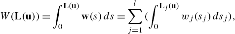
W(L(u))=∫L(u)0w(s)ds=l∑j=1(∫Lj(u)0wj(sj)dsj),
where w(s)=tanh−1(ˉL−1s)=[w1(s1)⋯wl(sl)]T![]() and ˉL
and ˉL![]() is the constant diagonal matrix given by ˉL=diag(ˉL1,...,ˉLl)
is the constant diagonal matrix given by ˉL=diag(ˉL1,...,ˉLl)![]() , which determines the bounds on L(u)
, which determines the bounds on L(u)![]() . Note that the bounds are originally given for the control input u(t)
. Note that the bounds are originally given for the control input u(t)![]() itself. However, one can transform these bounds to bounds on L(u)
itself. However, one can transform these bounds to bounds on L(u)![]() .
.
The H∞![]() control is to develop a control input such that (1) the system (1) with w=0
control is to develop a control input such that (1) the system (1) with w=0![]() is asymptotically stable and (2) the L2
is asymptotically stable and (2) the L2![]() gain condition (14.6) with z(t)
gain condition (14.6) with z(t)![]() defined in (14.36) is satisfied in the presence of w∈L2[0,∞)
defined in (14.36) is satisfied in the presence of w∈L2[0,∞)![]() .
.
The disturbance attenuation condition is satisfied if the following cost function is nonpositive:
J(X)=∫∞te−α(τ−t)[(X−r)TQ(X−r)+W(L(u))−γ2wTw]dτ.

14.3.3 Solution of the H∞ Control Tracking Problem of Nonaffine Systems
Define the tracking error as (14.3). Then, using (14.2) and (14.31), the tracking error dynamics becomes
˙ed(t)=˙X(t)−˙r(t)=f(X(t))+g(X(t))L(u)+Dw(t)−hd(r)(t).
Based on (14.2) and (14.38), an augmented system can be constructed in terms of the tracking error e(t)![]() and the reference trajectory r(t)
and the reference trajectory r(t)![]() as
as
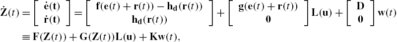
˙Z(t)=[˙e(t)˙r(t)]=[f(e(t)+r(t))−hd(r(t))hd(r(t))]+[g(e(t)+r(t))0]L(u)+[D0]w(t)≡F(Z(t))+G(Z(t))L(u)+Kw(t),
where the augmented state is
Z(t)=[e(t)r(t)].

The performance index (14.37) can be rewritten as
J(L(u),w)=∫∞te−α(τ−t)(ZT(τ)Q1Z(τ)+W(L(u))−γ2wTw)dτ,
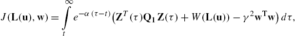
with Q1=[Q000]![]() .
.
The H∞![]() control problem can be expressed as a two-player zero-sum differential game in which the control effort policy player L(u)
control problem can be expressed as a two-player zero-sum differential game in which the control effort policy player L(u)![]() seeks to minimize the value function, while the disturbance policy player w(t)
seeks to minimize the value function, while the disturbance policy player w(t)![]() desires to maximize it. The goal is to find the feedback saddle point (L⋆(u),w⋆)
desires to maximize it. The goal is to find the feedback saddle point (L⋆(u),w⋆)![]() such that [42]
such that [42]
V⋆(Z(t))=minL(u)maxwJ(L(u),w).
On the basis of (14.40) and noting that V(Z(t))=J(L(u),w)![]() , the H∞
, the H∞![]() tracking Bellman equation is
tracking Bellman equation is
ZTQ1Z+W(L(u))−γ2wTw−αV(Z)+˙V(Z)=0
and the Hamiltonian is given by
H(Z,L(u),w,VZ)=ZTQ1Z+W(L(u))−γ2wTw−αV(Z)+VTZ(F(Z)+G(Z)L(u)+Kw).
Then the optimal control effort L(u)![]() and disturbance input w(t)
and disturbance input w(t)![]() for the given problem are obtained by employing the stationarity condition
for the given problem are obtained by employing the stationarity condition
L⋆(u)=argminL(u)H(Z,L(u),w,V⁎)≜d[ZTQ1Z+W(L(u))−γ2wTw−αV⋆+(V⋆Z)T˙Z]dL(u),w⋆=argmaxwH(Z,L(u),w,V⋆)≜d[ZTQ1Z+W(L(u))−γ2wTw−αV⋆+(V⋆Z)T˙Z]dw,

which give
L⋆(u)=−ˉLtanhT(v⋆),
w⋆=12γ−2(V⁎Z)TK,
where
v⋆=(V⋆Z)TG.
Substituting (14.43) and (14.44) in Bellman equation (14.42) yields the HJI equation
ZTQ1Z+W(L⋆(u))−γ2(w⋆)Tw⋆−αV⋆(Z)+˙V⋆(Z)=0.
To find the optimal control solution, the tracking HJI equation (14.46) could first be solved and then the control effort L⋆(u)![]() given by (14.43).
given by (14.43).
Note that the minimization problem (14.41) is defined in terms of L(u)![]() . Under certain conditions, this is equivalent to minimization in terms of u(t)
. Under certain conditions, this is equivalent to minimization in terms of u(t)![]() .
.
Lemma 2
We have minuH(Z,L(u),w,VZ)=minL(u)H(Z,L(u),w,VZ)![]() if the elements of L(u)
if the elements of L(u)![]() are independent.
are independent.
Proof
The minimum of H(Z,L(u),w,VZ)![]() with respect to u is equal to
with respect to u is equal to
minuH(Z,L(u),w,VZ)=(∂L(u)∂u)T∂H(Z,L(u),w,VZ)∂L(u)=0

and the minimum of H(Z,L(u),w,VZ)![]() with respect to L(u)
with respect to L(u)![]() is equal to
is equal to
minL(u)H(Z,L(u),w,VZ)=dH(Z,L(u),w,VZ)dL(u)=0.

Eqs. (14.47) and (14.48) are equivalent if and only if J=dL(u)/du![]() is a nonsingular matrix which guarantees the elements of L(u)
is a nonsingular matrix which guarantees the elements of L(u)![]() are independent [46]. □
are independent [46]. □
Note that if the elements of L⋆(u)![]() are independent, then the optimal control is given by
are independent, then the optimal control is given by
u⋆=−L−1(ˉLtanhT(v⋆)),
thus L(u⋆)=L⋆(u)![]() . Otherwise, it is shown in the subsequent sections how to use (14.43) to find v⋆
. Otherwise, it is shown in the subsequent sections how to use (14.43) to find v⋆![]() and u⋆
and u⋆![]() consequently to assure L(u⋆)=L⋆(u)
consequently to assure L(u⋆)=L⋆(u)![]() . The next result holds for both independent and dependent L(u)
. The next result holds for both independent and dependent L(u)![]() .
.
Theorem 2
Solution to bounded L2![]() gain problem
gain problem
If the elements of L(u)![]() are independent, then there exists a u⋆
are independent, then there exists a u⋆![]() such that L(u⋆)=L⋆(u)
such that L(u⋆)=L⋆(u)![]() and this u⋆
and this u⋆![]() makes the L2
makes the L2![]() gain less than or equal to γ. On the other hand, if the elements of L⋆(u)
gain less than or equal to γ. On the other hand, if the elements of L⋆(u)![]() are dependent, a method of solution is suggested in subsequent sections.
are dependent, a method of solution is suggested in subsequent sections.
14.3.4 Off-Policy Reinforcement Learning for Nonaffine Systems
In this section, the off-policy RL is presented to solve the optimal H∞![]() control of nonaffine nonlinear systems. In the proposed method, no knowledge about the system dynamics and the reference trajectory dynamics is needed. Moreover, it does not require an adjustable disturbance input and it avoids bias in finding the value function. Two algorithms are developed for two different cases: (1) for nonaffine systems with independent elements in L(u)
control of nonaffine nonlinear systems. In the proposed method, no knowledge about the system dynamics and the reference trajectory dynamics is needed. Moreover, it does not require an adjustable disturbance input and it avoids bias in finding the value function. Two algorithms are developed for two different cases: (1) for nonaffine systems with independent elements in L(u)![]() and (2) for nonaffine systems with dependent elements in L(u)
and (2) for nonaffine systems with dependent elements in L(u)![]() . Then the implementation of these two algorithms is given.
. Then the implementation of these two algorithms is given.
The system dynamics (14.39) can be rewritten as
˙Z(t)=F(Z(t))+G(Z(t))Lj(u)+Kwj+G(Z(t))(L(u)−Lj(u))+K(w−wj),
where Lj(u)![]() and wj(t)
and wj(t)![]() are the policies that are updated. By contrast, L(u)
are the policies that are updated. By contrast, L(u)![]() and w(t)
and w(t)![]() are the policies that are applied to the system to collect the data.
are the policies that are applied to the system to collect the data.
By the definition, it is easy to see that
e−α(tk−tk−1)Vj+1(Z(tk))−Vj+1(Z(tk−1))=∫tktk−1e−α(τ−tk−1)(Vj+1Z)T˙Z(t)−αVj+1dt.

Substituting (14.50) into (14.51) yields
e−α(tk−tk−1)Vj+1(Z(tk))−Vj+1(Z(tk−1))=∫tktk−1e−α(τ−tk−1)(Vj+1Z)T[F(Z(t))+G(Z(t))Lj(u)+Kwj+G(Z(t)(L(u)−Lj(u))+K(w−wj)]dt.

On the other hand, one has
(Vj+1Z)T[F(Z)+G(Z)Lj(u)+Kwj]=αVj+1−ra(Z(t),Lj(u),wj),
where
ra(Z(t),Lj(u),wj)=ZTQ1Z+W(L(uj))−γ2(wj)Twj.
Substituting (14.53) into (14.52) yields
e−α(tk−tk−1)Vj+1(Z(tk))−Vj+1(Z(tk−1))=∫tktk−1e−α(τ−tk−1)((Vj+1Z)T×[G(Z(t)(L(u)−Lj(u))+K(w−wj)]−ra(Z(t),Lj(u),wj))dt.
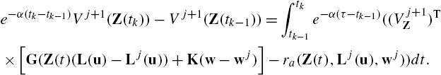
Using (14.43)–(14.45) in (14.54) yields the following off-policy H∞![]() Bellman equation:
Bellman equation:
e−α(tk−tk−1)Vj+1(Z(tk))−Vj+1(Z(tk−1))=∫tktk−1e−α(τ−tk−1)((vj+1ˉL(tanhT(vj)−tanhT(v))+2γ2wj+1(w−wj)−ra(Z(t),vj,wj))dt.

Note that if vj![]() and wj
and wj![]() are given, the unknown functions Vj+1(Z)
are given, the unknown functions Vj+1(Z)![]() , vj+1
, vj+1![]() and wj+1
and wj+1![]() can be approximated using (14.55). Then Lj+1(u)
can be approximated using (14.55). Then Lj+1(u)![]() is found from vj+1
is found from vj+1![]() .
.
The elements of Lj+1(u)![]() can be either dependent or independent. If elements in Lj+1(u)
can be either dependent or independent. If elements in Lj+1(u)![]() are independent, then the Bellman equation (14.55) can be solved iteratively using stored data to find L⋆(u)
are independent, then the Bellman equation (14.55) can be solved iteratively using stored data to find L⋆(u)![]() and the optimal control policy is u⋆
and the optimal control policy is u⋆![]() . The following algorithm shows how to iterate on (14.55) to find the optimal control policy in this case.
. The following algorithm shows how to iterate on (14.55) to find the optimal control policy in this case.
Algorithm 3 gives Lj+1(u)![]() and, if the condition of Lemma 2 is satisfied, then the elements of the control input are uj+1=−L−1(ˉLtanhT(vj+1))
and, if the condition of Lemma 2 is satisfied, then the elements of the control input are uj+1=−L−1(ˉLtanhT(vj+1))![]() . However, if elements in Lj+1(u)
. However, if elements in Lj+1(u)![]() are dependent, then the dependency of its elements must be taken into account by encoding equality constraints while solve Eq. (14.55) for vj+1
are dependent, then the dependency of its elements must be taken into account by encoding equality constraints while solve Eq. (14.55) for vj+1![]() .
.

To find a form for solution constraints L(u)![]() if it has dependent elements, consider the UAV system in Example 1 with
if it has dependent elements, consider the UAV system in Example 1 with
L(u(t))=[L1L2L3L4L5]=[u1u2u22u2cos(u3)u2sin(u3)].
Then, the dependency of the elements of L(u)![]() becomes
becomes
L3=L22=L42+L52.
This gives the following equality constraints:
ˉL3tanh(v3)=(ˉL2tanh(v2))2=(ˉL4tanh(v4))2+(ˉL5tanh(v5))2.
In general, it is seen that one has a vector of equality functions
f(L)=[f1(L),...,fp(L)]T=0,
with p being the number of dependent elements in L(u)![]() . For example for the UAV system, one has f1=ˉL3tanh(v3)−(ˉL2tanh(v2))2
. For example for the UAV system, one has f1=ˉL3tanh(v3)−(ˉL2tanh(v2))2![]() , f2=(ˉL2tanh(v2))2−(ˉL4tanh(v4))2−(ˉL5tanh(v5))2
, f2=(ˉL2tanh(v2))2−(ˉL4tanh(v4))2−(ˉL5tanh(v5))2![]() and f3=(ˉL3tanh(v3))−(ˉL4tanh(v4))2−(ˉL5tanh(v5))2
and f3=(ˉL3tanh(v3))−(ˉL4tanh(v4))2−(ˉL5tanh(v5))2![]() . This constraint must be taken into account when solving (14.55) for v using NNs.
. This constraint must be taken into account when solving (14.55) for v using NNs.
The following algorithm shows how to find the optimal control solution for the cases where L(u)![]() has dependent elements. The details of implementation of solving (14.55) for v while considering the constraint imposed by the independency of elements of v are presented in the next subsection.
has dependent elements. The details of implementation of solving (14.55) for v while considering the constraint imposed by the independency of elements of v are presented in the next subsection.
Before proceeding, ˉH![]() is defined as
is defined as
ˉH=∫tktk−1e−α(τ−tk−1)((vj+1ˉL(tanhT(vj)−tanhT(v))+2γ2wj+1(w−wj)−ra(Z(t),vj,wj))dt−e−α(tk−tk−1)Vj+1(Z(tk))+Vj+1(Z(tk−1)).

The minimum value of ˉH![]() in Algorithm 4 not considering the constraint (14.57) is zero. If this algorithm terminates, so that ˉH=0
in Algorithm 4 not considering the constraint (14.57) is zero. If this algorithm terminates, so that ˉH=0![]() , then by Theorem 2 the L2
, then by Theorem 2 the L2![]() gain problem is solved and there exists a u⋆
gain problem is solved and there exists a u⋆![]() such that L(u⋆)=L⋆(u)
such that L(u⋆)=L⋆(u)![]() .
.

The following subsection shows how to use NNs along with linear and nonlinear LS, respectively, to implement Algorithms 3 and 4.
14.3.5 Neural Networks for Implementation of Off-Policy RL Algorithms
In this subsection, the solution of the off-policy H∞![]() Bellman equations (14.56) and Eq. (14.58) in Algorithms 3 and 4 using three NNs is presented. The unknown functions Vj+1(Z)
Bellman equations (14.56) and Eq. (14.58) in Algorithms 3 and 4 using three NNs is presented. The unknown functions Vj+1(Z)![]() , vj+1
, vj+1![]() and wj+1
and wj+1![]() can be approximated by three NNs as
can be approximated by three NNs as
ˆVj+1(Z)=N1∑i=1ˆcj+1iϕi(Z)=ˆCj+1ϕ(Z),

ˆvij+1=N2∑k=1ˆpj+1i,kσi,k(Z)=ˆPij+1σi(Z),

ˆwij+1=N3∑k=1ˆqj+1i,kρi,k(Z)=ˆQij+1ρi(Z),

where ˆvj+1=[ˆv1j+1,...,ˆvlj+1]![]() , ˆwj+1=[ˆw1j+1,...,ˆwqj+1]
, ˆwj+1=[ˆw1j+1,...,ˆwqj+1]![]() . The terms ϕi(Z)=[ϕi1,...,ϕiNi1]
. The terms ϕi(Z)=[ϕi1,...,ϕiNi1]![]() , σi(Z)=[σi1,...,σiNi2]
, σi(Z)=[σi1,...,σiNi2]![]() and ρi(Z)=[ρi1,...,ρiN3]
and ρi(Z)=[ρi1,...,ρiN3]![]() are basis function vectors, ˆCj+1
are basis function vectors, ˆCj+1![]() , ˆPij+1
, ˆPij+1![]() and ˆQij+1
and ˆQij+1![]() are constant weight vectors and N1
are constant weight vectors and N1![]() , N2
, N2![]() and N3
and N3![]() are the number of neurons. Substituting (14.59)–(14.61) into the off-policy H∞
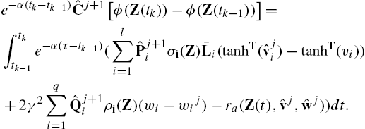
are the number of neurons. Substituting (14.59)–(14.61) into the off-policy H∞![]() Bellman equation (14.55) yields
Bellman equation (14.55) yields
e−α(tk−tk−1)ˆCj+1[ϕ(Z(tk))−ϕ(Z(tk−1))]=∫tktk−1e−α(τ−tk−1)(l∑i=1ˆPij+1σi(Z)ˉLi(tanhT(ˆvij)−tanhT(vi))+2γ2q∑i=1ˆQij+1ρi(Z)(wi−wij)−ra(Z(t),ˆvj,ˆwj))dt.
By defining ˆP=[ˆP1...ˆPl]![]() and ˆQ=[ˆQ1...ˆQq]
and ˆQ=[ˆQ1...ˆQq]![]() , Eq. (14.62) can be rewritten as
, Eq. (14.62) can be rewritten as
ˆWTh(tk)=y(tk),
where
ˆW=[(ˆCj+1)T(ˆPj+1)T(ˆQj+1)T]T,h(tk)=[e−α(tk−tk−1)ϕ(Z(tk))−ϕ(Z(tk−1))∫tktk−1e−α(τ−tk−1)σ1(Z)ˉL1(tanhT(ˆv1j)−tanhT(v1))dτ⋮∫tktk−1e−α(τ−tk−1)σl(Z)ˉLl(tanhT(ˆvlj)−tanhT(vl))dτ2γ2∫tktk−1e−α(τ−tk−1)ρ1(Z)(w1−w1j)dτ⋮2γ2∫tktk−1e−α(τ−tk−1)ρq(Z)(wq−wqj)dτ],y(tk)=∫tktk−1e−α(τ−tk−1)ra(Z(t),ˆvj,ˆwj))dt.

Case 1: Independency in Elements of L(u)![]() Eq. (14.63) can be solved using the least square method for parameter vector ˆW
Eq. (14.63) can be solved using the least square method for parameter vector ˆW![]() . Then the approximated value function and disturbance input are (14.59) and (14.61), respectively. The control input ˆuj+1
. Then the approximated value function and disturbance input are (14.59) and (14.61), respectively. The control input ˆuj+1![]() is found by determining L(ˆuj+1)
is found by determining L(ˆuj+1)![]() based on (14.45) from (14.60). The number of unknown parameters ˆW
based on (14.45) from (14.60). The number of unknown parameters ˆW![]() is N1+N2+N3
is N1+N2+N3![]() . Then, at least N⩾N1+N2+N3
. Then, at least N⩾N1+N2+N3![]() data sampled t1
data sampled t1![]() to tN
to tN![]() should be collect before solving (14.63) in the least square sense,
should be collect before solving (14.63) in the least square sense,
Y=[y(t1)...y(tN)]T,H=[h(t1)...h(tN)].

The least square solution is obtained as
ˆW=(HHT)−1HY.
Case 2: Dependency in Elements of L(u)![]() If the elements of L(u)
If the elements of L(u)![]() are dependent, one has to solve a constrained nonlinear least square problem to take into account the equality constraints imposed by the dependency of the elements of L(u)
are dependent, one has to solve a constrained nonlinear least square problem to take into account the equality constraints imposed by the dependency of the elements of L(u)![]() . To show this, consider the case of the UAV in Example 1. The following constraints are considered when finding the weights of NNs:
. To show this, consider the case of the UAV in Example 1. The following constraints are considered when finding the weights of NNs:
ˉL3tanh(ˆPj+13σ3(Z))=(ˉL2tanh(ˆPj+12σ2(Z)))2=(ˉL4tanh(ˆPj+14σ4(Z)))2+(ˉL5tanh(ˆPj+15σ5(Z)))2.

This constraint is nonlinear in NN weights and thus requires using the nonlinear least square method. In general, (14.58) becomes
argminˆW‖ˆWH−Y‖2s.t.f(ˆPj+1,σ1,...,σl)=0,

where the function f is defined in (14.57) and depends on how the elements of L(u)![]() and consequently NN weights are related.
and consequently NN weights are related.