Chapter 5 Thread Cooperation
We have now written our first program using CUDA C as well as have seen how to write code that executes in parallel on a GPU. This is an excellent start! But arguably one of the most important components to parallel programming is the means by which the parallel processing elements cooperate on solving a problem. Rare are the problems where every processor can compute results and terminate execution without a passing thought as to what the other processors are doing. For even moderately sophisticated algorithms, we will need the parallel copies of our code to communicate and cooperate. So far, we have not seen any mechanisms for accomplishing this communication between sections of CUDA C code executing in parallel. Fortunately, there is a solution, one that we will begin to explore in this chapter.
5.1 Chapter Objectives
Through the course of this chapter, you will accomplish the following:
• You will learn about what CUDA C calls threads.
• You will learn a mechanism for different threads to communicate with each other.
• You will learn a mechanism to synchronize the parallel execution of different threads.
5.2 Splitting Parallel Blocks
In the previous chapter, we looked at how to launch parallel code on the GPU. We did this by instructing the CUDA runtime system on how many parallel copies of our kernel to launch. We call these parallel copies blocks.
The CUDA runtime allows these blocks to be split into threads. Recall that when we launched multiple parallel blocks, we changed the first argument in the angle brackets from 1 to the number of blocks we wanted to launch. For example, when we studied vector addition, we launched a block for each element in the vector of size N by calling this:
add<<<N,1>>>( dev_a, dev_b, dev_c );
Inside the angle brackets, the second parameter actually represents the number of threads per block we want the CUDA runtime to create on our behalf. To this point, we have only ever launched one thread per block. In the previous example, we launched the following:
N blocks x 1 thread/block = N parallel threads
So really, we could have launched N/2 blocks with two threads per block, N/4 blocks with four threads per block, and so on. Let’s revisit our vector addition example armed with this new information about the capabilities of CUDA C.
5.2.1 Vector Sums: Redux
We endeavor to accomplish the same task as we did in the previous chapter. That is, we want to take two input vectors and store their sum in a third output vector. However, this time we will use threads instead of blocks to accomplish this.
You may be wondering, what is the advantage of using threads rather than blocks? Well, for now, there is no advantage worth discussing. But parallel threads within a block will have the ability to do things that parallel blocks cannot do. So for now, be patient and humor us while we walk through a parallel thread version of the parallel block example from the previous chapter.
GPU Vector Sums Using Threads
We will start by addressing the two changes of note when moving from parallel blocks to parallel threads. Our kernel invocation will change from one that launches N blocks of one thread apiece:
add<<<N,1>>>( dev_a, dev_b, dev_c );
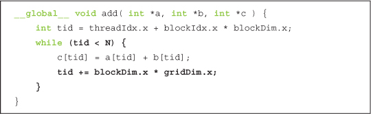
to a version that launches N threads, all within one block:
add<<<1,N>>>( dev_a, dev_b, dev_c );
The only other change arises in the method by which we index our data. Previously, within our kernel we indexed the input and output data by block index.
![]()
The punch line here should not be a surprise. Now that we have only a single block, we have to index the data by thread index.
![]()
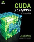
These are the only two changes required to move from a parallel block implementation to a parallel thread implementation. For completeness, here is the entire source listing with the changed lines in bold:
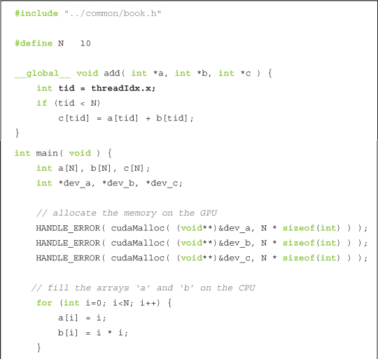
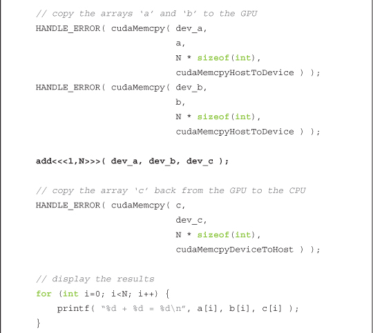
Pretty simple stuff, right? In the next section, we’ll see one of the limitations of this thread-only approach. And of course, later we’ll see why we would even bother splitting blocks into other parallel components.
GPU Sums of a Longer Vector
In the previous chapter, we noted that the hardware limits the number of blocks in a single launch to 65,535. Similarly, the hardware limits the number of threads per block with which we can launch a kernel. Specifically, this number cannot exceed the value specified by the maxThreadsPerBlock field of the device properties structure we looked at in Chapter 3. For many of the graphics processors currently available, this limit is 512 threads per block, so how would we use a thread-based approach to add two vectors of size greater than 512? We will have to use a combination of threads and blocks to accomplish this.
As before, this will require two changes: We will have to change the index computation within the kernel, and we will have to change the kernel launch itself.
Now that we have multiple blocks and threads, the indexing will start to look similar to the standard method for converting from a two-dimensional index space to a linear space.
![]()
This assignment uses a new built-in variable, blockDim. This variable is a constant for all blocks and stores the number of threads along each dimension of the block. Since we are using a one-dimensional block, we refer only to blockDim.x. If you recall, gridDim stored a similar value, but it stored the number of blocks along each dimension of the entire grid. Moreover, gridDim is two-dimensional, whereas blockDim is actually three-dimensional. That is, the CUDA runtime allows you to launch a two-dimensional grid of blocks where each block is a three-dimensional array of threads. Yes, this is a lot of dimensions, and it is unlikely you will regularly need the five degrees of indexing freedom afforded you, but they are available if so desired.
Indexing the data in a linear array using the previous assignment actually is quite intuitive. If you disagree, it may help to think about your collection of blocks of threads spatially, similar to a two-dimensional array of pixels. We depict this arrangement in Figure 5.1.
Figure 5.1 A two-dimensional arrangement of a collection of blocks and threads
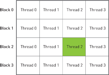
If the threads represent columns and the blocks represent rows, we can get a unique index by taking the product of the block index with the number of threads in each block and adding the thread index within the block. This is identical to the method we used to linearize the two-dimensional image index in the Julia Set example.
![]()
Here, DIM is the block dimension (measured in threads), y is the block index, and x is the thread index within the block. Hence, we arrive at the index: tid = threadIdx.x + blockIdx.x * blockDim.x.
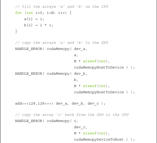
The other change is to the kernel launch itself. We still need N parallel threads to launch, but we want them to launch across multiple blocks so we do not hit the 512-thread limitation imposed upon us. One solution is to arbitrarily set the block size to some fixed number of threads; for this example, let’s use 128 threads per block. Then we can just launch N/128 blocks to get our total of N threads running.
The wrinkle here is that N/128 is an integer division. This implies that if N were 127, N/128 would be zero, and we will not actually compute anything if we launch zero threads. In fact, we will launch too few threads whenever N is not an exact multiple of 128. This is bad. We actually want this division to round up.
There is a common trick to accomplish this in integer division without calling ceil(). We actually compute (N+127)/128 instead of N/128. Either you can take our word that this will compute the smallest multiple of 128 greater than or equal to N or you can take a moment now to convince yourself of this fact.
We have chosen 128 threads per block and therefore use the following kernel launch:
![]()
Because of our change to the division that ensures we launch enough threads, we will actually now launch too many threads when N is not an exact multiple of 128. But there is a simple remedy to this problem, and our kernel already takes care of it. We have to check whether a thread’s offset is actually between 0 and N before we use it to access our input and output arrays:

Thus, when our index overshoots the end of our array, as will always happen when we launch a nonmultiple of 128, we automatically refrain from performing the calculation. More important, we refrain from reading and writing memory off the end of our array.
GPU Sums of Arbitrarily Long Vectors
We were not completely forthcoming when we first discussed launching parallel blocks on a GPU. In addition to the limitation on thread count, there is also a hardware limitation on the number of blocks (albeit much greater than the thread limitation). As we’ve mentioned previously, neither dimension of a grid of blocks may exceed 65,535.
So, this raises a problem with our current vector addition implementation. If we launch N/128 blocks to add our vectors, we will hit launch failures when our vectors exceed 65,535 * 128 = 8,388,480 elements. This seems like a large number, but with current memory capacities between 1GB and 4GB, the high-end graphics processors can hold orders of magnitude more data than vectors with 8 million elements.
Fortunately, the solution to this issue is extremely simple. We first make a change to our kernel.
This looks remarkably like our original version of vector addition! In fact, compare it to the following CPU implementation from the previous chapter:
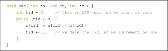
Here we also used a while() loop to iterate through the data. Recall that we claimed that rather than incrementing the array index by 1, a multi-CPU or multicore version could increment by the number of processors we wanted to use. We will now use that same principle in the GPU version.
In the GPU implementation, we consider the number of parallel threads launched to be the number of processors. Although the actual GPU may have fewer (or more) processing units than this, we think of each thread as logically executing in parallel and then allow the hardware to schedule the actual execution. Decoupling the parallelization from the actual method of hardware execution is one of the burdens that CUDA C lifts off a software developer’s shoulders. This should come as a relief, considering current NVIDIA hardware can ship with anywhere between 8 and 480 arithmetic units per chip!
Now that we understand the principle behind this implementation, we just need to understand how we determine the initial index value for each parallel thread and how we determine the increment. We want each parallel thread to start on a different data index, so we just need to take our thread and block indexes and linearize them as we saw in the “GPU Sums of a Longer Vector” section. Each thread will start at an index given by the following:
![]()
After each thread finishes its work at the current index, we need to increment each of them by the total number of threads running in the grid. This is simply the number of threads per block multiplied by the number of blocks in the grid, or blockDim.x * gridDim.x. Hence, the increment step is as follows:
tid += blockDim.x * gridDim.x;
We are almost there! The only remaining piece is to fix the launch itself. If you remember, we took this detour because the launch add<<<(N+127)/128,128>>>( dev_a, dev_b, dev_c ) will fail when (N+127)/128 is greater than 65,535. To ensure we never launch too many blocks, we will just fix the number of blocks to some reasonably small value. Since we like copying and pasting so much, we will use 128 blocks, each with 128 threads.
add<<<128,128>>>( dev_a, dev_b, dev_c );
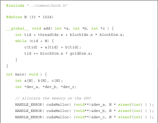
You should feel free to adjust these values however you see fit, provided that your values remain within the limits we’ve discussed. Later in the book, we will discuss the potential performance implications of these choices, but for now it suffices to choose 128 threads per block and 128 blocks. Now we can add vectors of arbitrary length, limited only by the amount of RAM we have on our GPU. Here is the entire source listing:
5.2.2 GPU Ripple Using Threads
As with the previous chapter, we will reward your patience with vector addition by presenting a more fun example that demonstrates some of the techniques we’ve been using. We will again use our GPU computing power to generate pictures procedurally. But to make things even more interesting, this time we will animate them. But don’t worry, we’ve packaged all the unrelated animation code into helper functions so you won’t have to master any graphics or animation.
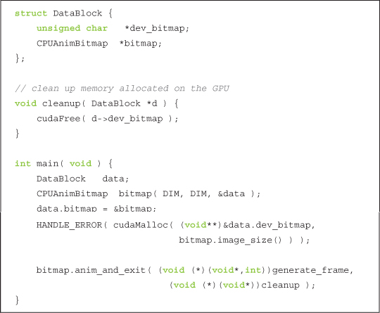
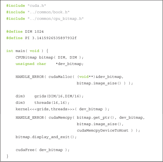
Most of the complexity of main() is hidden in the helper structure CPUAnimBitmap. You will notice that we again have a pattern of doing a cudaMalloc(), executing device code that uses the allocated memory, and then cleaning up with cudaFree(). This should be old hat to you by now.
In this example, we have slightly convoluted the means by which we accomplish the middle step, “executing device code that uses the allocated memory.” We pass the anim_and_exit() method a function pointer to generate_frame(). This function will be called by the structure every time it wants to generate a new frame of the animation.
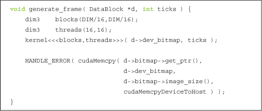
Although this function consists only of four lines, they all involve important CUDA C concepts. First, we declare two two-dimensional variables, blocks and threads. As our naming convention makes painfully obvious, the variable blocks represents the number of parallel blocks we will launch in our grid. The variable threads represents the number of threads we will launch per block. Because we are generating an image, we use two-dimensional indexing so that each thread will have a unique (x,y) index that we can easily put into correspondence with a pixel in the output image. We have chosen to use blocks that consist of a 16 x 16 array of threads. If the image has DIM x DIM pixels, we need to launch DIM/16 x DIM/16 blocks to get one thread per pixel. Figure 5.2 shows how this block and thread configuration would look in a (ridiculously) small, 48-pixel-wide, 32-pixel-high image.
Figure 5.2 A 2D hierarchy of blocks and threads that could be used to process a 48 x 32 pixel image using one thread per pixel
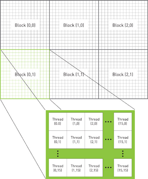
If you have done any multithreaded CPU programming, you may be wondering why we would launch so many threads. For example, to render a full high-definition animation at 1920 x 1080, this method would create more than 2 million threads. Although we routinely create and schedule this many threads on a GPU, one would not dream of creating this many threads on a CPU. Because CPU thread management and scheduling must be done in software, it simply cannot scale to the number of threads that a GPU can. Because we can simply create a thread for each data element we want to process, parallel programming on a GPU can be far simpler than on a CPU.
After declaring the variables that hold the dimensions of our launch, we simply launch the kernel that will compute our pixel values.
kernel<<< blocks, threads>>>( d->dev_bitmap, ticks );
The kernel will need two pieces of information that we pass as parameters. First, it needs a pointer to device memory that holds the output pixels. This is a global variable that had its memory allocated in main(). But the variable is “global” only for host code, so we need to pass it as a parameter to ensure that the CUDA runtime will make it available for our device code.
Second, our kernel will need to know the current animation time so it can generate the correct frame. The current time, ticks, is passed to the generate_frame() function from the infrastructure code in CPUAnimBitmap, so we can simply pass this on to our kernel.
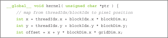
And now, here’s the kernel code itself:
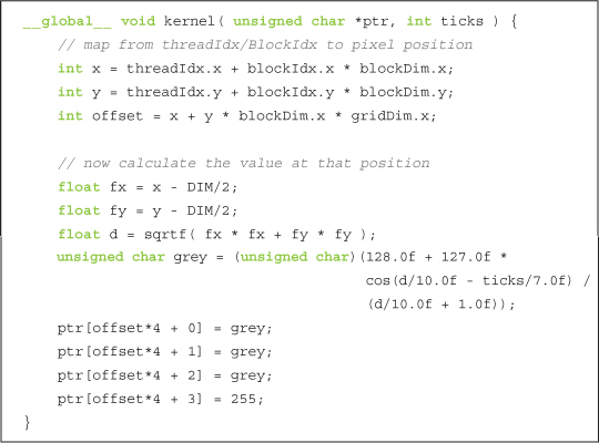
The first three are the most important lines in the kernel.
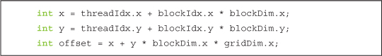
In these lines, each thread takes its index within its block as well as the index of its block within the grid, and it translates this into a unique (x,y) index within the image. So when the thread at index (3, 5) in block (12, 8) begins executing, it knows that there are 12 entire blocks to the left of it and 8 entire blocks above it. Within its block, the thread at (3, 5) has three threads to the left and five above it. Because there are 16 threads per block, this means the thread in question has the following:
3 threads + 12 blocks * 16 threads/block = 195 threads to the left of it
5 threads + 8 blocks * 16 threads/block = 128 threads above it
This computation is identical to the computation of x and y in the first two lines and is how we map the thread and block indices to image coordinates. Then we simply linearize these x and y values to get an offset into the output buffer. Again, this is identical to what we did in the “GPU Sums of a Longer Vector” and “GPU Sums of Arbitrarily Long Vectors” sections.
int offset = x + y * blockDim.x * gridDim.x;
Since we know which (x,y) pixel in the image the thread should compute and we know the time at which it needs to compute this value, we can compute any function of (x,y,t) and store this value in the output buffer. In this case, the function produces a time-varying sinusoidal “ripple.”
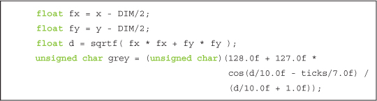
We recommend that you not get too hung up on the computation of grey. It’s essentially just a 2D function of time that makes a nice rippling effect when it’s animated. A screenshot of one frame should look something like Figure 5.3.
Figure 5.3 A screenshot from the GPU ripple example

5.3 Shared Memory and Synchronization
So far, the motivation for splitting blocks into threads was simply one of working around hardware limitations to the number of blocks we can have in flight. This is fairly weak motivation, because this could easily be done behind the scenes by the CUDA runtime. Fortunately, there are other reasons one might want to split a block into threads.
CUDA C makes available a region of memory that we call shared memory. This region of memory brings along with it another extension to the C language akin to __device__ and __global__. As a programmer, you can modify your variable declarations with the CUDA C keyword __shared__ to make this variable resident in shared memory. But what’s the point?
We’re glad you asked. The CUDA C compiler treats variables in shared memory differently than typical variables. It creates a copy of the variable for each block that you launch on the GPU. Every thread in that block shares the memory, but threads cannot see or modify the copy of this variable that is seen within other blocks. This provides an excellent means by which threads within a block can communicate and collaborate on computations. Furthermore, shared memory buffers reside physically on the GPU as opposed to residing in off-chip DRAM. Because of this, the latency to access shared memory tends to be far lower than typical buffers, making shared memory effective as a per-block, software-managed cache or scratchpad.
The prospect of communication between threads should excite you. It excites us, too. But nothing in life is free, and interthread communication is no exception. If we expect to communicate between threads, we also need a mechanism for synchronizing between threads. For example, if thread A writes a value to shared memory and we want thread B to do something with this value, we can’t have thread B start its work until we know the write from thread A is complete. Without synchronization, we have created a race condition where the correctness of the execution results depends on the nondeterministic details of the hardware.
Let’s take a look at an example that uses these features.
5.3.1 Dot Product
Congratulations! We have graduated from vector addition and will now take a look at vector dot products (sometimes called an inner product). We will quickly review what a dot product is, just in case you are unfamiliar with vector mathematics (or it has been a few years). The computation consists of two steps. First, we multiply corresponding elements of the two input vectors. This is very similar to vector addition but utilizes multiplication instead of addition. However, instead of then storing these values to a third, output vector, we sum them all to produce a single scalar output.
For example, if we take the dot product of two four-element vectors, we would get Equation 5.1.
![]()
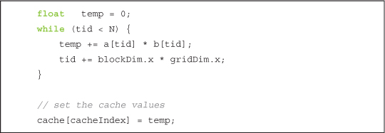
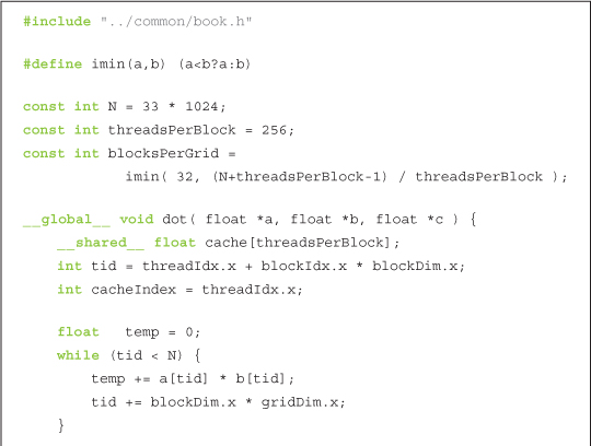
Perhaps the algorithm we tend to use is becoming obvious. We can do the first step exactly how we did vector addition. Each thread multiplies a pair of corresponding entries, and then every thread moves on to its next pair. Because the result needs to be the sum of all these pairwise products, each thread keeps a running sum of the pairs it has added. Just like in the addition example, the threads increment their indices by the total number of threads to ensure we don’t miss any elements and don’t multiply a pair twice. Here is the first step of the dot product routine:
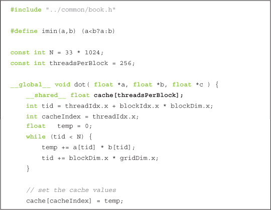
As you can see, we have declared a buffer of shared memory named cache. This buffer will be used to store each thread’s running sum. Soon we will see why we do this, but for now we will simply examine the mechanics by which we accomplish it. It is trivial to declare a variable to reside in shared memory, and it is identical to the means by which you declare a variable as static or volatile in standard C:
__shared__float cache[threadsPerBlock];
We declare the array of size threadsPerBlock so each thread in the block has a place to store its temporary result. Recall that when we have allocated memory globally, we allocated enough for every thread that runs the kernel, or threadsPerBlock times the total number of blocks. But since the compiler will create a copy of the shared variables for each block, we need to allocate only enough memory such that each thread in the block has an entry.
After allocating the shared memory, we compute our data indices much like we have in the past:
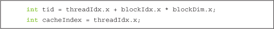
The computation for the variable tid should look familiar by now; we are just combining the block and thread indices to get a global offset into our input arrays. The offset into our shared memory cache is simply our thread index. Again, we don’t need to incorporate our block index into this offset because each block has its own private copy of this shared memory.
Finally, we clear our shared memory buffer so that later we will be able to blindly sum the entire array without worrying whether a particular entry has valid data stored there:
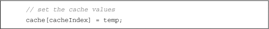
It will be possible that not every entry will be used if the size of the input vectors is not a multiple of the number of threads per block. In this case, the last block will have some threads that do nothing and therefore do not write values.
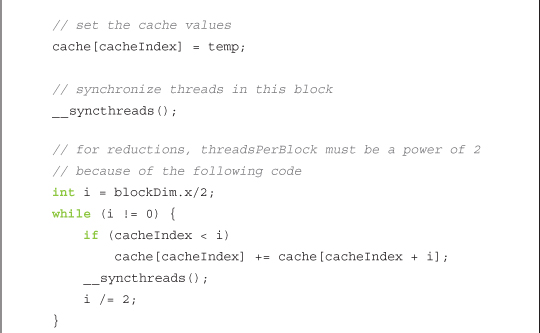
Each thread computes a running sum of the product of corresponding entries in a and b. After reaching the end of the array, each thread stores its temporary sum into the shared buffer.
At this point in the algorithm, we need to sum all the temporary values we’ve placed in the cache. To do this, we will need some of the threads to read the values that have been stored there. However, as we mentioned, this is a potentially dangerous operation. We need a method to guarantee that all of these writes to the shared array cache[] complete before anyone tries to read from this buffer. Fortunately, such a method exists:
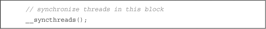
This call guarantees that every thread in the block has completed instructions prior to the __syncthreads() before the hardware will execute the next instruction on any thread. This is exactly what we need! We now know that when the first thread executes the first instruction after our __syncthreads(), every other thread in the block has also finished executing up to the __syncthreads().
Now that we have guaranteed that our temporary cache has been filled, we can sum the values in it. We call the general process of taking an input array and performing some computations that produce a smaller array of results a reduction. Reductions arise often in parallel computing, which leads to the desire to give them a name.
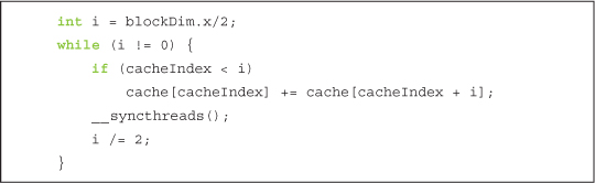
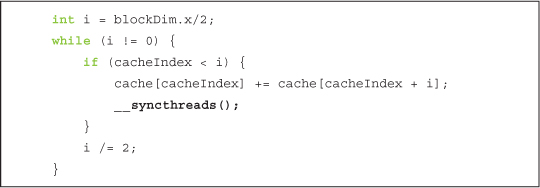
The naïve way to accomplish this reduction would be having one thread iterate over the shared memory and calculate a running sum. This will take us time proportional to the length of the array. However, since we have hundreds of threads available to do our work, we can do this reduction in parallel and take time that is proportional to the logarithm of the length of the array. At first, the following code will look convoluted; we’ll break it down in a moment.
The general idea is that each thread will add two of the values in cache[] and store the result back to cache[]. Since each thread combines two entries into one, we complete this step with half as many entries as we started with. In the next step, we do the same thing on the remaining half. We continue in this fashion for log2(threadsPerBlock) steps until we have the sum of every entry in cache[]. For our example, we’re using 256 threads per block, so it takes 8 iterations of this process to reduce the 256 entries in cache[] to a single sum.
The code for this follows:
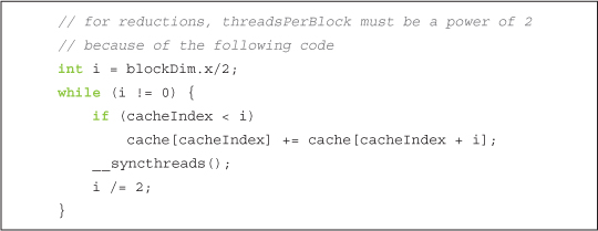
Figure 5.4 One step of a summation reduction
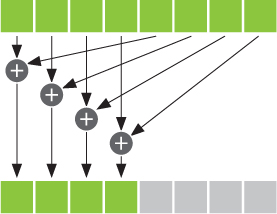
For the first step, we start with i as half the number of threadsPerBlock. We only want the threads with indices less than this value to do any work, so we conditionally add two entries of cache[] if the thread’s index is less than i. We protect our addition within an if(cacheIndex < i) block. Each thread will take the entry at its index in cache[], add it to the entry at its index offset by i, and store this sum back to cache[].
Suppose there were eight entries in cache[] and, as a result, i had the value 4. One step of the reduction would look like Figure 5.4.
After we have completed a step, we have the same restriction we did after computing all the pairwise products. Before we can read the values we just stored in cache[], we need to ensure that every thread that needs to write to cache[] has already done so. The __syncthreads() after the assignment ensures this condition is met.
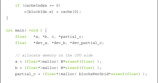
After termination of this while() loop, each block has but a single number remaining. This number is sitting in the first entry of cache[] and is the sum of every pairwise product the threads in that block computed. We then store this single value to global memory and end our kernel:
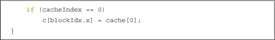
Why do we do this global store only for the thread with cacheIndex == 0? Well, since there is only one number that needs writing to global memory, only a single thread needs to perform this operation. Conceivably, every thread could perform this write and the program would still work, but doing so would create an unnecessarily large amount of memory traffic to write a single value. For simplicity, we chose the thread with index 0, though you could conceivably have chosen any cacheIndex to write cache[0] to global memory. Finally, since each block will write exactly one value to the global array c[], we can simply index it by blockIdx.
We are left with an array c[], each entry of which contains the sum produced by one of the parallel blocks. The last step of the dot product is to sum the entries of c[]. Even though the dot product is not fully computed, we exit the kernel and return control to the host at this point. But why do we return to the host before the computation is complete?
Previously, we referred to an operation like a dot product as a reduction. Roughly speaking, this is because we produce fewer output data elements than we input. In the case of a dot product, we always produce exactly one output, regardless of the size of our input. It turns out that a massively parallel machine like a GPU tends to waste its resources when performing the last steps of a reduction, since the size of the data set is so small at that point; it is hard to utilize 480 arithmetic units to add 32 numbers!
For this reason, we return control to the host and let the CPU finish the final step of the addition, summing the array c[]. In a larger application, the GPU would now be free to start another dot product or work on another large computation. However, in this example, we are done with the GPU.
In explaining this example, we broke with tradition and jumped right into the actual kernel computation. We hope you will have no trouble understanding the body of main() up to the kernel call, since it is overwhelmingly similar to what we have shown before.
To avoid you passing out from boredom, we will quickly summarize this code:
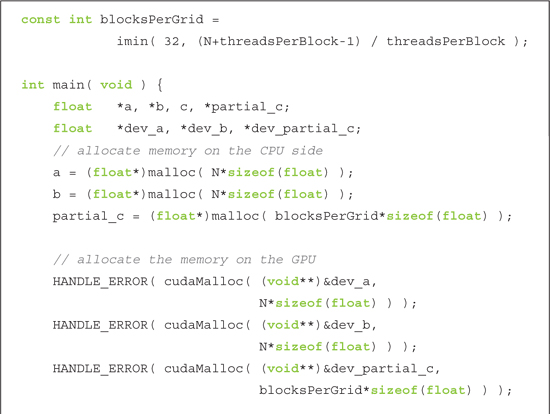
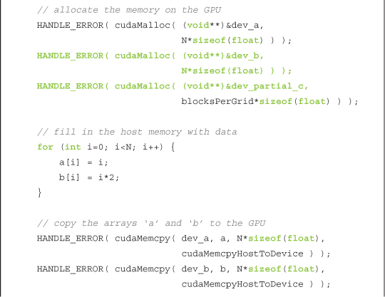
1. Allocate host and device memory for input and output arrays.
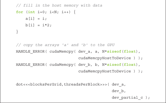
2. Fill input arrays a[] and b[], and then copy these to the device using cudaMemcpy().
3. Call our dot product kernel using some predetermined number of threads per block and blocks per grid.
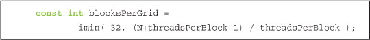
Despite most of this being commonplace to you now, it is worth examining the computation for the number of blocks we launch. We discussed how the dot product is a reduction and how each block launched will compute a partial sum. The length of this list of partial sums should be something manageably small for the CPU yet large enough such that we have enough blocks in flight to keep even the fastest GPUs busy. We have chosen 32 blocks, although this is a case where you may notice better or worse performance for other choices, especially depending on the relative speeds of your CPU and GPU.
But what if we are given a very short list and 32 blocks of 256 threads apiece is too many? If we have N data elements, we need only N threads in order to compute our dot product. So in this case, we need the smallest multiple of threadsPerBlock that is greater than or equal to N. We have seen this once before when we were adding vectors. In this case, we get the smallest multiple of threadsPerBlock that is greater than or equal to N by computing (N+(threadsPerBlock-1)) / threadsPerBlock. As you may be able to tell, this is actually a fairly common trick in integer math, so it is worth digesting this even if you spend most of your time working outside the CUDA C realm.
Therefore, the number of blocks we launch should be either 32 or (N+(threadsPerBlock-1)) / threadsPerBlock, whichever value is smaller.
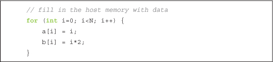
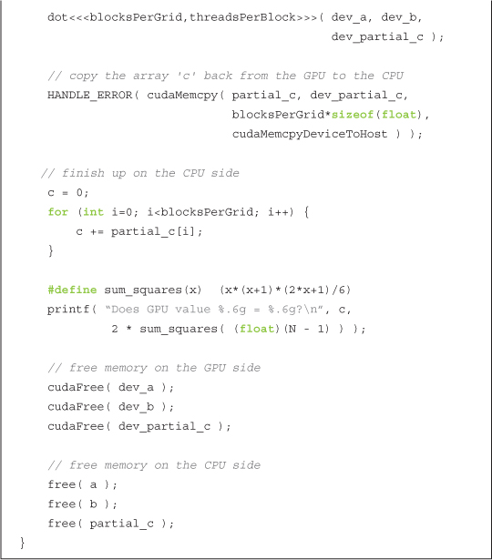
Now it should be clear how we arrive at the code in main(). After the kernel finishes, we still have to sum the result. But like the way we copy our input to the GPU before we launch a kernel, we need to copy our output back to the CPU before we continue working with it. So after the kernel finishes, we copy back the list of partial sums and complete the sum on the CPU.
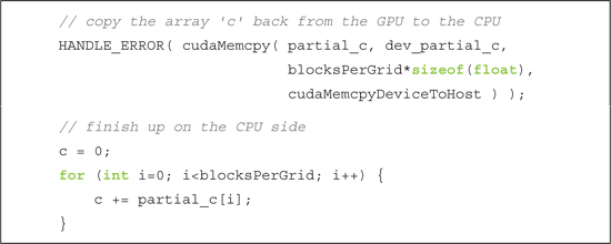
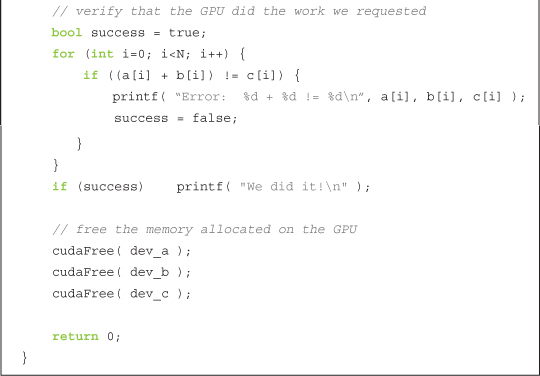
Finally, we check our results and clean up the memory we’ve allocated on both the CPU and GPU. Checking the results is made easier because we’ve filled the inputs with predictable data. If you recall, a[] is filled with the integers from 0 to N-1 and b[] is just 2*a[].
Our dot product should be two times the sum of the squares of the integers from 0 to N-1. For the reader who loves discrete mathematics (and what’s not to love?!), it will be an amusing diversion to derive the closed-form solution for this summation. For those with less patience or interest, we present the closed-form here, as well as the rest of the body of main():
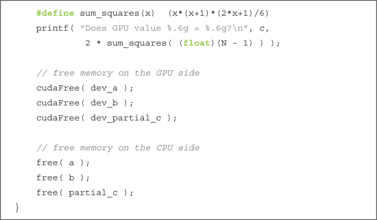
If you found all our explanatory interruptions bothersome, here is the entire source listing, sans commentary:
5.3.2 Dot Product Optimized (Incorrectly)
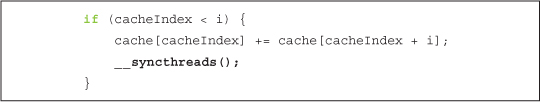
We quickly glossed over the second __syncthreads() in the dot product example. Now we will take a closer look at it as well as examining an attempt to improve it. If you recall, we needed the second __syncthreads() because we update our shared memory variable cache[] and need these updates to be visible to every thread on the next iteration through the loop.
Observe that we update our shared memory buffer cache[] only if cacheIndex is less than i. Since cacheIndex is really just threadIdx.x, this means that only some of the threads are updating entries in the shared memory cache. Since we are using __syncthreads only to ensure that these updates have taken place before proceeding, it stands to reason that we might see a speed improvement if we wait only for the threads that are actually writing to shared memory. We do this by moving the synchronization call inside the if() block:
Although this was a valiant effort at optimization, it will not actually work. In fact, the situation is worse than that. This change to the kernel will actually cause the GPU to stop responding, forcing you to kill your program. But what could have gone so catastrophically wrong with such a seemingly innocuous change?
To answer this question, it helps to imagine every thread in the block marching through the code one line at a time. At each instruction in the program, every thread executes the same instruction, but each can operate on different data. But what happens when the instruction that every thread is supposed to execute is inside a conditional block like an if()? Obviously not every thread should execute that instruction, right? For example, consider a kernel that contains the following fragment of code that intends for odd-indexed threads to update the value of some variable:
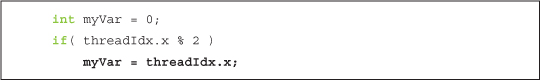
In the previous example, when the threads arrive at the line in bold, only the threads with odd indices will execute it since the threads with even indices do not satisfy the condition if( threadIdx.x % 2 ). The even-numbered threads simply do nothing while the odd threads execute this instruction. When some of the threads need to execute an instruction while others don’t, this situation is known as thread divergence. Under normal circumstances, divergent branches simply result in some threads remaining idle, while the other threads actually execute the instructions in the branch.
But in the case of __syncthreads(), the result is somewhat tragic. The CUDA Architecture guarantees that no thread will advance to an instruction beyond the __syncthreads() until every thread in the block has executed the __syncthreads(). Unfortunately, if the __syncthreads() sits in a divergent branch, some of the threads will never reach the __syncthreads(). Therefore, because of the guarantee that no instruction after a __syncthreads() can be executed before every thread has executed it, the hardware simply continues to wait for these threads. And waits. And waits. Forever.
This is the situation in the dot product example when we move the __syncthreads() call inside the if() block. Any thread with cacheIndex greater than or equal to i will never execute the __syncthreads(). This effectively hangs the processor because it results in the GPU waiting for something that will never happen.
The moral of this story is that __syncthreads() is a powerful mechanism for ensuring that your massively parallel application still computes the correct results. But because of this potential for unintended consequences, we still need to take care when using it.
5.3.3 Shared Memory Bitmap
We have looked at examples that use shared memory and employed __syncthreads() to ensure that data is ready before we continue. In the name of speed, you may be tempted to live dangerously and omit the __syncthreads(). We will now look at a graphical example that requires __syncthreads() for correctness. We will show you screenshots of the intended output and of the output when run without __syncthreads(). It won’t be pretty.
The body of main() is identical to the GPU Julia Set example, although this time we launch multiple threads per block:
As with the Julia Set example, each thread will be computing a pixel value for a single output location. The first thing that each thread does is compute its x and y location in the output image. This computation is identical to the tid computation in the vector addition example, although we compute it in two dimensions this time:
Since we will be using a shared memory buffer to cache our computations, we declare one such that each thread in our 16 x 16 block has an entry.
__shared__ float shared[16][16];
Then, each thread computes a value to be stored into this buffer.

And lastly, we store these values back out to the pixel, reversing the order of x and y:

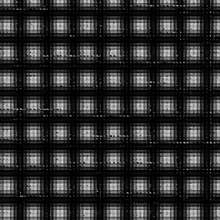
Granted, these computations are somewhat arbitrary. We’ve simply come up with something that will draw a grid of green spherical blobs. So after compiling and running this kernel, we output an image like the one in Figure 5.5.
What happened here? As you may have guessed from the way we set up this example, we’re missing an important synchronization point. When a thread stores the computed value in shared[][] to the pixel, it is possible that the thread responsible for writing that value to shared[][] has not finished writing it yet. The only way to guarantee that this does not happen is by using __syncthreads(). Thus, the result is a corrupted picture of green blobs.
Figure 5.5 Ascreenshot rendered without proper synchronization
Although this may not be the end of the world, your application might be computing more important values.
Instead, we need to add a synchronization point between the write to shared memory and the subsequent read from it.
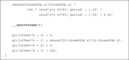
With this __syncthreads() in place, we then get a far more predictable (and aesthetically pleasing) result, as shown in Figure 5.6.
Figure 5.6 A screenshot after adding the correct synchronization

5.4 Chapter Review
We know how blocks can be subdivided into smaller parallel execution units known as threads. We revisited the vector addition example of the previous chapter to see how to perform addition of arbitrarily long vectors. We also showed an example of reduction and how we use shared memory and synchronization to accomplish this. In fact, this example showed how the GPU and CPU can collaborate on computing results. Finally, we showed how perilous it can be to an application when we neglect the need for synchronization.
You have learned most of the basics of CUDA C as well as some of the ways it resembles standard C and a lot of the important ways it differs from standard C. This would be an excellent time to consider some of the problems you have encountered and which ones might lend themselves to parallel implementations with CUDA C. As we progress, we will look at some of the other features we can use to accomplish tasks on the GPU, as well as some of the more advanced API features that CUDA provides to us.