Chapter 5 Bending of Beams

5.1. Introduction

In this chapter we are concerned with the bending of straight as well as curved beams—that is, structural elements possessing one dimension significantly greater than the other two, usually loaded in a direction normal to the longitudinal axis.

Except in the case of very simple shapes and loading systems, the theory of elasticity yields beam solutions only with considerable difficulty. Practical considerations often lead to assumptions with regard to stress and deformation that result in mechanics of materials or elementary theory solutions. The theory of elasticity can sometimes be applied to test the validity of such assumptions. The role of the theory of elasticity is then threefold. It can serve to place limitations on the use of the elementary theory, it can be used as the basis of approximate solutions through numerical analysis, and it can provide exact solutions when configurations of loading and shape are simple.

Part A—Exact Solutions

5.2. Pure Bending of Beams of Symmetrical Cross Section

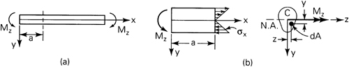
The simplest case of pure bending is that of a beam possessing a vertical axis of symmetry, subjected to equal and opposite end couples (Fig. 5.1a). The semi-inverse method is now applied to analyze this problem. The moment M_z shown in the figure is defined as positive, because it acts on a positive (negative) face with its vector in the positive (negative) coordinate direction. This sign convention agrees with that of stress (Sec. 1.4). We shall assume that the normal stress over the cross section varies linearly with y and that the remaining stress components are zero:

Figure 5.1. Beam of singly symmetric cross section in pure bending.

(5.1)

Here k is a constant, and y = 0 contains the neutral surface, that is, the surface along which σ_x = 0. The intersection of the neutral surface and the cross section locates the neutral axis (abbreviated N.A.). Figure 5.1b shows the linear stress field in a section located an arbitrary distance a from the left end.

Since Eqs. (5.1) indicate that the lateral surfaces are free of stress, we need only be assured that the stresses are consistent with the boundary conditions at the ends. These conditions require that the resultant of the internal forces be zero and that the moments of the internal forces about the neutral axis equal the applied moment M_z:

(5.2)

where A is the cross-sectional area. It should be noted that the zero stress components τ_xy, τ_xz in Eqs. (5.1) satisfy the conditions that no y- and z-directed forces exist at the end faces, and because of the y symmetry of the section, σ_x = ky produces no moment about the y axis. The negative sign in the second expression implies that a positive moment M_z is one that results in compressive (negative) stress at points of positive y. Substitution of Eqs. (5.1) into Eqs. (5.2) yields

(5-3a,b)

Inasmuch as k ≠ 0, Eq. (5.3a) indicates that the first moment of cross-sectional area about the neutral axis is zero. This requires that the neutral and centroidal axes of the cross section coincide. Neglecting body forces, it is clear that the equations of equilibrium (3.4), are satisfied by Eqs. (5.1). It may readily be verified also that Eqs. (5.1) together with Hooke’s law fulfill the compatibility conditions, Eq. (2.9). Thus, Eqs. (5.1) represent an exact solution.

The integral in Eq. (5.3b) defines the moment of inertia I_z of the cross section about the z axis of the beam cross section (Appendix C); therefore

(a)

An expression for normal stress can now be written by combining Eqs. (5.1) and (a):

(5-4)

This is the familiar elastic flexure formula applicable to straight beams.

Since, at a given section, M and I are constant, the maximum stress is obtained from Eq. (5.4) by taking |y|_max = c:

(5-5)

Here S is the elastic section modulus. Formula (5.5) is widely employed in practice because of its simplicity. To facilitate its use, section moduli for numerous common sections are tabulated in various handbooks. A fictitious stress in extreme fibers, computed from Eq. (5.5) for experimentally obtained ultimate bending moment (Sec. 12.6), is termed the modulus of rupture of the material in bending. This, σ_max = M_u/S, is frequently used as a measure of the bending strength of materials.

Kinematic Relationships

To gain further insight into the beam problem, consideration is now given to the geometry of deformation, that is, beam kinematics. Fundamental to this discussion is the hypothesis that sections originally plane remain so subsequent to bending. For a beam of symmetrical cross section, Hooke’s law and Eq. (5.4) lead to

(5-6)

where EI_Z is the flexural rigidity.

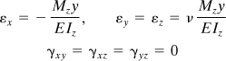
Let us examine the deflection of the beam axis, the axial deformation of which is zero. Figure 5.2a shows an element of an initially straight beam, now in a deformed state. Because the beam is subjected to pure bending, uniform throughout, each element of infinitesimal length experiences identical deformation, with the result that the beam curvature is everywhere the same. The deflected axis of the beam or the deflection curve is thus shown deformed, with radius of curvature r_x. The curvature of the beam axis in the xy plane in terms of the y deflection υ is

(5-7)

Figure 5.2. Segment of a bent beam.

where the approximate form is valid for small deformations (dv/dx << 1). The sign convention for curvature of the beam axis is such that it is positive when the beam is bent concave downward as shown in the figure. From the geometry of Fig. 5.2b, the shaded sectors are similar. Hence, the radius of curvature and the strain are related as follows:

(5-8)

Here ds is the arc length mn along the longitudinal axis of the beam. For small displacement, ds ≈ dx, and θ represents the slope dv/dx of the beam axis. Clearly, for the positive curvature shown, θ increases as we move from left to right along the beam axis. On the basis of Eqs. (5.6) and (5.8),

(5-9a)

Following a similar procedure and noting that ε_z ≈ –νε_x, we may also obtain the curvature in the yz plane as

(5-9b)

The basic beam equation is obtained by combining Eqs. (5.7) and (5.9a) as follows:

(5-10)

This expression, relating the beam curvature to the bending moment, is known as the Bernoulli-Euler law of elementary bending theory. It is observed from Fig. 5.2 and Eq. (5.10) that a positive moment produces positive curvature. If the sign convention adopted in this section for either moment or deflection (and curvature) should be reversed, the plus sign in Eq. (5.10) should likewise be reversed.

Reference to Fig. 5.2a reveals that the top and bottom lateral surfaces have been deformed into saddle-shaped or anticlastic surfaces of curvature 1/r_z. The vertical sides have been simultaneously rotated as a result of bending. Examining Eq. (5.9b) suggests a method for determining Poisson’s ratio [Ref. 5.1]. For a given beam and bending moment, a measurement of 1/r_z leads directly to v. The effect of anticlastic curvature is small when the beam depth is comparable to its width.

5.3. Pure Bending of Beams of Asymmetrical Cross Section

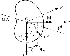
The development of Sec. 5.2 is now extended to the more general case in which a beam of arbitrary cross section is subjected to end couples M_y and M_z about the y and z axes, respectively (Fig. 5.3). Following a procedure similar to that of Sec. 5.2, plane sections are again taken to remain plane. Assume that the normal stress σ_x acting at a point within dA is a linear function of the y and z coordinates of the point; assume further that the remaining stresses are zero. The stress field is thus

(5-11)

Figure 5.3. Pure bending of beams of asymmetrical cross section.

where c₁, c₂, c₃ are constants to be evaluated.

The conditions at the beam ends, as before, relate to the force and bending moment:

(a)

(b,c)

Substitution of σ_x, as given by Eq. (5.11), into Eqs. (a), (b), and (c) results in the following expressions:

(d)

(e)

(f)

For the origin of the y and z axes to be coincident with the centroid of the section, it is required that

(g)

We conclude, therefore, from Eq. (d) that c₁ = 0, and from Eqs. (5.11) that σ_x = 0 at the origin. The neutral axis is thus observed to pass through the centroid, as in the beam of symmetrical section. It may be verified that the field of stress described by Eqs. (5.11) satisfies the equations of equilibrium and compatibility and that the lateral surfaces are free of stress. Now consider the defining relationships

(5.12)

where I_y and I_z are the moments of inertia about the y and z axes, respectively, and I_yz is the product of inertia about the y and z axes. From Eqs. (e) and (f), together with Eqs. (5.12), we obtain expressions for c₂ and c₃.

Substitution of the constants into Eqs. (5.11) results in the following generalized flexure formula:

(5.13)

The equation of the neutral axis is found by equating this expression to zero:

(5.14)

This is an inclined line through the centroid C. The angle ϕ between the neutral axis and the z axis is determined as follows:

(5.15)

The angle Φ (measured from the z axis) is positive in the clockwise direction, as shown in Fig. 5.3. The highest bending stress occurs at a point located farthest from the neutral axis.

There is a specific orientation of the y and z axes for which the product of inertia I_yz vanishes. Labeling the axes so oriented y′ and z′, we have I_y′z′ = 0. The flexure formula under these circumstances becomes

(5.16)

The y′ and z′ axes now coincide with the principal axes of inertia of the cross section. The stresses at any point can now be ascertained by applying Eq. (5.13) or (5.16).

The kinematic relationships discussed in Sec. 5.2 are valid for beams of asymmetrical section provided that y and z represent principal axes.

Recall that the two-dimensional stress (or strain) and the moment of inertia of an area are second-order tensors (Appendix A). Thus, the transformation equations for stress and moment of inertia are analogous (Sec. C.4). The Mohr’s circle analysis and all conclusions drawn for stress therefore apply to the moment of inertia. With reference to the coordinate axes shown in Fig. 5.3, applying Eq. (C.12a), the moment of inertia about the y′ axis is found to be

(5.17)

From Eq. (C.13) the orientation of the principal axes is given by

(5.18)

The principal moment of inertia, I₁ and I₂, from Eq. (C.14) are

(5.19)

Subscripts 1 and 2 refer to the maximum and minimum values, respectively.

Determination of the moments of inertia and stresses in an asymmetrical section will now be illustrated.

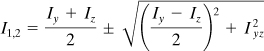
Example 5.1

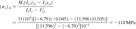
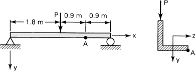
A 150- by 150-mm slender angle of 20-mm thickness is subjected to oppositely directed end couples M_z = 11 kN · m, at the centroid of the cross section. What bending stresses exist at points A and B on a section away from the ends (Fig. 5.4a)? Determine the orientation of the neutral axis.

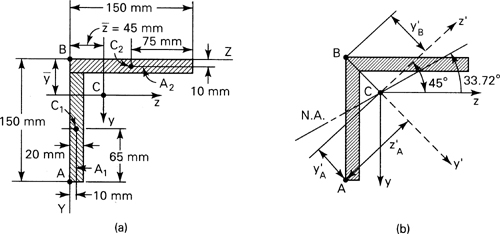
Figure 5.4. Example 5.1.

Solution Equations (5.13) and (5.16) will be applied to ascertain the normal stress. This requires first the determination of a number of section properties, through the use of familiar expressions of mechanics given in Appendix C. Note that the FORTRAN computer program presented in Table C.2 provides a check of the numerical values obtained here for the area characteristics and may easily be extended to compute the stresses.

Location of the Centroid C. Let and represent the distances from C to arbitrary reference lines (denoted Z and Y):

Here represents the z distance from the Y reference line to the centroid of each subarea (A₁ and A₂) composing the total cross section. Since the section is symmetrical, = .

Moments and Products of Inertia. For a rectangular section of depth h and width b, the moment of inertia about the neutral axis is I = bh³/12 (Table C.1). We now use yz axes as reference axes through C. Representing the distances from C to the centroids of each subarea by d_y1, d_y2, d_z1, and d_z2, we obtain the moments of inertia with respect to these axes using the parallel-axis theorem. Applying Eq. (C.9),

Thus, referring to Fig. 5.4a,

The transfer formula (C.11) for a product of inertia yields

Stresses Using Formula (5.13). We have y_A = 0.105 m, y_B = –0.045 m, Z_A = –0.045 m, Z_B = –0.045 m, and M_y = 0. Thus,

(h)

Similarly,

Alternatively, these stresses may be calculated by proceeding as follows.

Directions of the Principal Axes and the Principal Moments of Inertia. Employing Eq. (5.18), we have

Therefore, the two values of θ_p are 45° and 135°. Substituting the first of these values into Eq. (5.17), we obtain I_y′ = [11.596 + 6.79 sin 90°]10⁶ = 18.386 × 10⁶ mm⁴. Since the principal moments of inertia are, by application of Eq. (5.19),

it is observed that I₁ = I_y′ = 18.386 × 10⁶ mm⁴ and I₂ = I_z′ = 4.806 × 10⁶ mm⁴. The principal axes are indicated in Fig. 5.4b as the y′z′ axes.

Stresses Using Formula (5.16). The components of bending moment about the principal axes are

M_y′ = 11(10³) sin 45° = 7778 N·m

M_z′ = 11(10³) cos 45° = 7778 N·m

Equation (5.16) is now applied, referring to Fig. 5.4b, with y′_A = 0.043 m, z′_A = −0.106 m, , and z′_B = 0, determined from geometrical considerations:

as before.

Direction of the Neutral Axis. From Eq. (5.15), with M_y = 0,

The negative sign indicates that the neutral is located counterclockwise from the z axis (Fig. 5.4b).

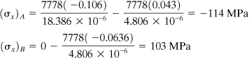
5.4. Bending of a Cantilever of Narrow Section

Consider a narrow cantilever beam of rectangular cross section, loaded at its free end by a concentrated force of such magnitude that the beam weight may be neglected (Fig. 5.5). The situation described may be regarded as a case of plane stress provided that the beam thickness t is small relative to beam depth 2 h. The distribution of stress in the beam, as we have already found in Example 3.1, is given by

(3-21)

Figure 5.5. Deflections of an end-loaded cantilever beam.

To derive expressions for the beam displacement, it is necessary to relate stress, described by Eq. (3.21), to strain. This is accomplished through the use of the strain–displacement relations and Hooke’s law:

(a,b)

(c)

Integration of Eqs. (a) and (b) yields

(d)

(e)

Differentiating Eqs. (d) and (e) with respect to y and x, respectively, and substituting into Eq. (c), we have

In this expression, note that the left and right sides depend only on y and x, respectively. These variables are independent of one another, and it is therefore concluded that the equation can be valid only if each side is equal to the same constant:

These are integrated to yield

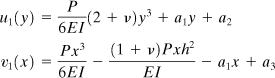
in which a₂ and a₃ are constants of integration. The displacements may now be written

(5.20a)

(5.20b)

The constants a₁, a₂, and a₃ depend on known conditions. If, for example, the situation at the fixed end is such that

then, from Eqs. (5.20),

The beam displacement is therefore

(5.21)

(5.22)

It is clear on examining these equations that u and v do not obey a simple linear relationship with y and x. We conclude, therefore, that plane sections do not, as assumed in elementary theory, remain plane subsequent to bending.

The vertical displacement of the beam axis is obtained by substituting y = 0 into Eq. (5.22):

(5.23)

Introducing the foregoing into Eq. (5.7), the radius of curvature is given by

provided that dυ/dx is a small quantity. Once again we obtain Eq. (5.9a), the beam curvature-moment relationship of elementary bending theory.

It is also a simple matter to compare the total vertical deflection at the free end (x = 0) with the deflection derived in elementary theory. Substituting x = 0 into Eq. (5.23), the total deflection is

(5.24)

wherein the deflection associated with shear is clearly Ph²L/2GI = 3PL/2GA. The ratio of the shear deflection to the bending deflection at x = 0 provides a measure of beam slenderness:

If, for example, L = 10(2h), the preceding quotient is only . For a slender beam, 2h << L, and it is clear that the deflection is mainly due to bending. It should be mentioned here, however, that in vibration at higher modes, and in wave propagation, the effect of shear is of great importance in slender as well as in other beams.

In the case of wide beams (t >> 2h), Eq. (5.24) must be modified by replacing E and v as indicated in Table 3.1.

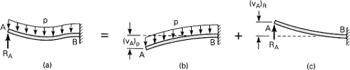
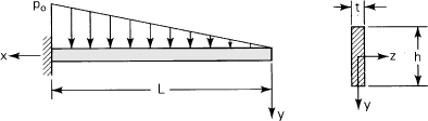
5.5. Bending of a Simply Supported, Narrow Beam

Consideration is now given to the stress distribution in a narrow beam of thickness t and depth 2h subjected to a uniformly distributed loading (Fig. 5.6). The situation as described is one of plane stress, subject to the following boundary conditions, consistent with the origin of an x, y coordinate system located at midspan and midheight of the beam, as shown:

(a)

>Figure 5.6. Bending of a simply supported beam with a uniform load.

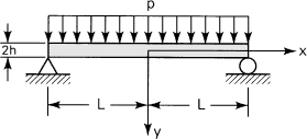
Since at the ends no longitudinal load is applied, it would appear reasonable to state that σ_x = 0 at x = ±L. However, this boundary condition leads to a complicated solution, and a less severe statement is instead used:

(b)

The corresponding condition for bending couples at x = ±L is

(c)

For y equilibrium, it is required that

(d)

The problem is treated by superimposing the solutions Φ₂, Φ₃, and Φ₅ (Sec. 3.6), with

c₂ = b₂ = a₃ = c₃ = a₅ = b₅ = c₅ = e₅ = 0

We then have

The stresses are

(e)

The conditions (a) are

and the solution is

The constant d₃ is obtained from condition (c) as follows:

or

Expressions (e) together with the values obtained for the constants also fulfill conditions (b) and (d).

The state of stress is thus represented by

(5.25a)

(5.25b)

(5.25c)

Here is the area moment of inertia taken about a line through the centroid, parallel to the z axis. Although the solutions given by Eqs. (5.25) satisfy the equations of elasticity and the boundary conditions, they are nevertheless not exact. This is indicated by substituting x = ±L into Eq. (5.25a) to obtain the following expression for the normal distributed forces per unit area at the ends:

which cannot exist, as no forces act at the ends. From Saint-Venant’s principle we may conclude, however, that the solutions do predict the correct stresses throughout the beam, except near the supports.

Recall that the longitudinal normal stress derived from elementary beam theory is σ_x = –My/I; this is equivalent to the first term of Eq. (5.25a). The second term is then the difference between the longitudinal stress results given by the two approaches. To gauge the magnitude of the deviation, consider the ratio of the second term of Eq. (5.25a) to the result of elementary theory at x = 0. At this point, the bending moment is a maximum. Substituting y = h for the condition of maximum stress, we obtain

For a beam of length 10 times its depth, the ratio is small, . For beams of ordinary proportions, we can conclude that elementary theory provides a result of sufficient accuracy for σ_x. As for σ_y, this stress is not found in the elementary theory. The result for τ_xy is, on the other hand, the same as that of elementary beam theory.

The displacement of the beam may be determined in a manner similar to that described for a cantilever beam (Sec. 5.4).

Part B—Approximate Solutions

5.6. Elementary Theory of Bending

We may conclude, on the basis of the previous sections, that exact solutions are difficult to obtain. It was also observed that for a slender beam the results of the exact theory do not differ markedly from that of the mechanics of materials or elementary approach provided that solutions close to the ends are not required. The bending deflection was found to be very much larger than the shear deflection. Thus, the stress associated with the former predominates. We deduce therefore that the normal strain ε_y resulting from transverse loading may be neglected. Because it is more easily applied, the elementary approach is usually preferred in engineering practice. The exact and elementary theories should be regarded as complementary rather than competitive approaches, enabling the analyst to obtain the degree of accuracy required in the context of the specific problem at hand.

The basic assumptions of the elementary theory, for a slender beam whose cross section is symmetrical about the vertical plane of loading, are

(5.26)

(5.27)

The first equation of (5.26) is equivalent to the assertion υ = υ(x). Thus, all points in a beam at a given longitudinal location x experience identical deformation. The second equation of (5.26), together with υ = υ(x), yields, after integration,

(a)

The third equation of (5.26) and Eqs. (5.27) imply that the beam is considered narrow, and we have a case of plane stress.

At y = 0, the bending deformation should vanish. Referring to Eq. (a), it is clear, therefore, that u₀(x) must represent axial deformation. The term dυ/dx is the slope θ of the beam axis, as shown in Fig. 5.7a, and is very much smaller than unity. Therefore,

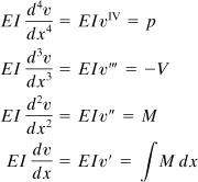
Figure 5.7. (a) Longitudinal displacements in a beam due to rotation of a plane section; (b) element between adjoining sections of a beam.

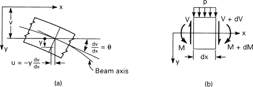
The slope is positive when clockwise, provided that the x and y axes have the directions shown. Since u is a linear function of y, this equation restates the kinematic hypothesis of the elementary theory of bending: Plane sections perpendicular to the longitudinal axis of the beam remain plane subsequent to bending. This assumption is confirmed by the exact theory only in the case of pure bending.

In the next section, we will obtain the stress distribution in a beam according to the elementary theory. We now derive some useful relations involving the shear force V, the bending moment M, the load per unit length p, the slope θ, and the deflection υ. Consider a beam element of length dx subjected to a distributed loading (Fig. 5.7b). Note that as dx is small the variation in the load per unit length p is omitted. In the free-body diagram, all the forces and the moments are positive. The shear force obeys the sign convention discussed in Sec. 1.4; the bending moment is in agreement with the convention adopted in Sec. 5.2. In general, the shear force and bending moment vary with the distance x, and it thus follows that these quantities will have different values on each face of the element. The increments in shear force and bending moment are denoted by dV and dM, respectively. Equilibrium of forces in the vertical direction is governed by V − (V + dV) − pdx = 0, or

(5.28)

That is, the rate of change of shear force with respect to x is equal to the algebraic value of the distributed loading. Equilibrium of the moments about a z axis through the left end of the element, neglecting the higher-order infinitesimals, leads to

(5.29)

This relation states that the rate of change of bending moment is equal to the algebraic value of the shear force, valid only if a distributed load or no load acts on the beam segment. Combining Eqs. (5.28) and (5.29), we have

(5.30)

The basic equation of bending of a beam, Eq. (5.10), combined with Eq. (5.30), may now be written as

(5.31)

For a beam of constant flexural rigidity EI, the beam equations derived here may be expressed as

(5.32)

These relationships also apply to wide beams provided that E/(1 – v²) is substituted for E (Table 3.1).

In many problems of practical importance, the deflection due to transverse loading of a beam may be obtained through successive integration of the beam equation:

(5.33)

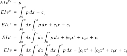
Alternatively, we could begin with EIυ″ = M(x) and integrate twice to obtain

(5.34)

In either case, the constants, c₁, c₂, c₃, and c₄, which correspond to the homogeneous solution of the differential equations, may be evaluated from the boundary conditions. The constants c₁, c₂, c₃/EI, and c₄/EI represent the values at the origin of V, M, θ, and ν, respectively. In the method of successive integration, there is no need to distinguish between statically determinate and statically indeterminate systems (Sec. 5.11), because the equilibrium equations represent only two of the boundary conditions (on the first two integrals), and because the total number of boundary conditions is always equal to the total number of unknowns.

Example 5.2

A cantilever beam AB of length L and constant flexural rigidity EI carries a moment M₀ at its free end A (Fig. 5.8a). Derive the equation of the deflection curve and determine the slope and deflection at A.

Figure 5.8. Example 5.2

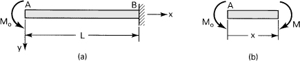
Solution From the free-body diagram of Fig. 5.8b, observe that the bending moment is +M₀ throughout the beam. Thus, the third of Eqs. (5.32) becomes

EIυ″ = M₀

Integrating, we obtain

EIυ′ = M₀x + c₁

The constant of integration c₁ can be found from the condition that the slope is zero at the support; therefore, we have υ′(L) = 0, from which c₁ = – M₀L. The slope is then

(5.35)

Integrating, we obtain

The boundary condition on the deflection at the support is υ(L) = 0, which yields c₂ = M₀L²/2EI. The equation of the deflection curve is thus a parabola:

(5.36)

However, every element of the beam experiences equal moments and deforms alike. The deflection curve should therefore be part of a circle. This inconsistancy results from the use of an approximation for the curvature, Eq. (5.7). The error is very small when, however, the deformation υ is small [Ref. 5.1].

The slope and deflection at A are readily found by letting x = 0 into Eqs. (5.35) and (5.36):

(5.37)

The minus sign indicates that the angle of rotation is counterclockwise (Fig. 5.8a).

5.7. Bending and Shear Stress

When a beam is bent by transverse loads, usually both a bending moment M and a shear force V act on each cross section. The distribution of the normal stress associated with the bending moment is given by the flexure formula, Eq. (5.4):

(5.38)

where M and I are taken with respect to the z axis (Fig. 5.7).

In accordance with the assumptions of elementary bending, Eqs. (5.26) and (5.27), the contribution of the shear strains to beam deformation is omitted. However, shear stresses do exist, and the shearing forces are the resultant of the stresses. The shearing stress τ_xy acting at section mn, assumed uniformly distributed over the area b·dx, can be determined on the basis of equilibrium of forces acting on the shaded part of the beam element (Fig. 5.9). Here b is the width of the beam a distance y₁ from the neutral axis and dx is the length of the element. The distribution of normal stresses produced by M and M + dM is indicated in the figure. The normal force distributed over the left face mr on the shaded area A^* is equal to

(a)

Figure 5.9. Element for analyzing beam shearing stress.

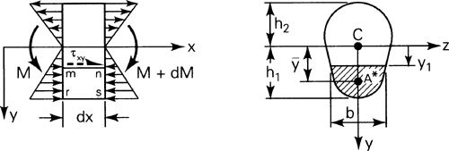
Similarly, an expression for the normal force on the right face ns may be written in terms of M + dM. The equilibrium of x-directed forces acting on the beam element is governed by

from which we have

Upon substitution of Eq. (5.29), we obtain the shear stress formula for beams:

(5.39)

The integral represented by Q is the first moment of the shaded area A^* with respect to the neutral axis z:

(5.40)

By definition, is the distance from the neutral axis to the centroid of A^*, In the case of sections of regular geometry, A^* provides a convenient means of calculating Q. Note that the shear force acting across the width of the beam per unit length q = τ_xy b = VQ/I is called the Shear flow.

For example, in the case of a rectangular cross section of width b and depth 2h, the shear stress at y₁ is

(5.41)

This shows that the shear stress varies parabolically with y₁; it is zero when y₁ = ±h and has its maximum value at the neutral axis, y₁ = 0:

(5.42)

Here, 2bh is the area of the rectangular cross section. It is observed that the maximum shear stress (either horizontal or vertical: τ_xy = τ_yx) is 1.5 times larger than the average shear stress V/A. As observed in Sec. 5.4, for a thin rectangular beam, (5.42) is the exact distribution of shear stress. However, in general, for wide rectangular sections and for other sections, Eq. (5.39) yields only approximate values of the shearing stress.

It should be pointed out that the maximum shear stress does not always occur at the neutral axis. For instance, in the case of a cross section having nonparallel sides, such as a triangular section, the maximum value of Q/b (and thus τ_xy) takes place at midheight, h/2, while the neutral axis is located at a distance h/3 from the base.

The following sample problem illustrates the application of the shear stress formula.

Example 5.3

A cantilever wide-flange beam is loaded by a force P at the free end acting through the centroid of the section. The beam is of constant thickness t (Fig. 5.10a). Determine the shear stress distribution in the section.

Figure 5.10. Example 5.3. Shearing stresses in a wide-flange beam.

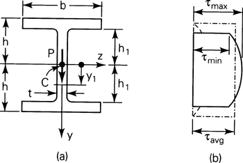
Solution The vertical shear force at every section is P. It is assumed that the shear stress τ_xy is uniformly distributed over the web thickness. Then, in the web, for 0 ≤ y₁ ≤ h₁, applying Eq. (5.39),

This equation may be written as

(b)

The shearing stress thus varies parabolically in the web (Fig. 5.10b). The extreme values of τ_xy found at y₁ = 0 and y₁ = ±h₁, are, from Eq. (b), as follows:

Note that it is usual that t << b, and therefore the maximum and minimum stresses do not differ appreciably, as is seen in the figure. Similarly, the shear stress in the flange, for h₁ < y₁ ≤ h, is

(c)

This is the parabolic equation for the variation of stress in the flange, shown by the dashed lines in the figure.

Clearly, for a thin flange, the shear stress is very small as compared with the shear stress in the web. It is concluded that the approximate average value of shear stress in the beam may be found by dividing P by the web cross section with the web height assumed equal to the beam overall height: τ_avg = P/2th. The preceding is indicated by the dotted lines in the figure. The distribution of stress given by Eq. (c) is fictitious, because the inner planes of the flanges must be free of shearing stress, as they are load-free boundaries of the beam. This contradiction cannot be resolved by the elementary theory; the theory of elasticity must be applied to obtain the correct solution. Fortunately, this defect of the shearing stress formula does not lead to serious error since, as pointed out previously, the web carries almost all the shear force. To reduce the stress concentration at the juncture of the web and the flange, the sharp corners should be rounded.

5.8. Effect of Transverse Normal Stress

When a beam is subjected to a transverse load, there will be a resulting transverse normal stress. According to Eq. (5.26), this stress is not related to the normal strain ε_y and thus cannot be determined from Hooke’s law. However, an expression for the average transverse normal stress can be obtained from the equilibrium requirement of force balance along the axis of the beam. For this purpose, a procedure is used similar to that employed for determining the shear stress in Sec. 5.7.

Consider, for example, a rectangular cantilever beam of width b and depth 2h subject to a uniform load of intensity p (Fig. 5.11a). The free-body diagram of an isolated beam segment of length dx is shown in Fig. 5.11b. Passing a horizontal plane through this segment results in the free-body diagram of Fig. 5.11c, for which the condition of statics ∑ F_y = 0 yields

(a)

Figure 5.11. Stresses in a uniformly loaded cantilever beam of rectangular cross section.

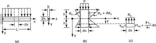
Here, the shear stress is defined by Eq. (5.41), as

(b)

Upon substitution of Eqs. (5.28) and (b) into Eq. (a), we have

Integration yields the transverse normal stress in the form

(5.43)

We see that this stress varies as a cubic parabola from –p/b at the surface (y = –h), where the load acts, to zero at the opposite surface (y = h).

The distribution of the bending and the shear stresses in a uniformly loaded cantilever beam (Fig. 5.11a) is determined from Eqs. (5.38) and (b):

(5.44)

The largest values of the σ_x, τ_xy, and σ_y given by Eqs. (5.43) and (5.44) are

(c)

To compare the magnitudes of the maximum stresses, consider the ratios

(d,e)

Because L is much greater than h in most beams, L ≥ 20h, it is observed from the preceding that the shear and the transverse normal stresses will usually be orders of magnitude smaller than the bending stresses. This is justification for assuming γ_xy = 0 and ε_y = 0 in the technical theory of bending. Note that Eq. (e) results in even smaller values than Eq. (d). Therefore, in practice it is reasonable to neglect σ_y.

The foregoing conclusion applies, in most cases, to beams of a variety of cross-sectional shapes and under various load configurations. Clearly, the factor of proportionality in Eqs. (d) and (e) will differ for beams of different sectional forms and for different loadings of a given beam.

5.9. Composite Beams

Beams constructed of two or more materials having different moduli of elasticity are referred to as composite beams. Examples include multilayer beams made by bonding together multiple sheets, sandwich beams consisting of high-strength material faces separated by a relatively thick layer of low-strength material such as plastic foam, and reinforced concrete beams. The assumptions of the technical theory for a homogeneous beam (Sec. 5.6) are valid for a beam of more than one material.

We shall employ the common transformed-section method to analyze a composite beam. In this technique, the cross section of several materials is transformed into an equivalent cross section of one material on which the resisting forces and the neutral axis are the same as on the original section. The usual flexure formula is then applied to the new section. To illustrate the method, a frequently used beam with a symmetrical cross section built of two different materials is considered (Fig. 5.12a).

Figure 5.12. Composite beam of two materials: (a) cross section; (b) strain distribution; (c) stress distribution; (d) transformed section.

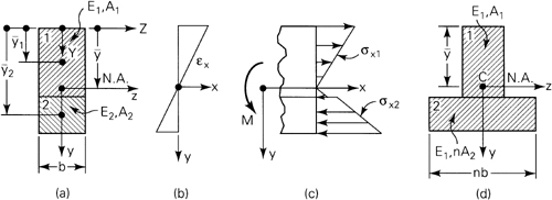
The cross sections of the beam remain plane during bending. It follows that the normal strain ε_x varies linearly with the distance y from the neutral axis of the section; that is, ε_x = ky (Figs. 5.12a and b). The location of the neutral axis is yet to be determined. Both materials of the beam are assumed to obey Hooke’s law, and their moduli of elasticity are designated E₁ and E₂. Then, the stress-strain relation gives

(5.45a,b)

This result is sketched in Fig. 5.12c for the assumption that E₂ > E₁. We introduce the notation

(5.46)

where n is called the modular ratio. Note that n > 1 in Eq. (5.46). However, this choice is arbitrary; the technique applies as well for n < 1.

Referring to the cross section (Figs. 5.12a and c), equilibrium equations ∑F_X = 0 and ∑M_z = 0 lead to

(a)

(b)

wherein A₁ and A₂ denote the cross-sectional areas for materials 1 and 2, respectively. Substituting into Eq. (a) σ_x1, σ_x2, and n as given by Eqs. (5.45) and (5.46) results in

(5.47)

Electing the top of the section as a reference (Fig. 5.12a), from Eq. (5.47) with y = Y – ,

or, setting

we have

The foregoing yields an alterative form of Eq. (5.47):

(5.47′)

Expression (5.47) or (5.47′) can be used to locate the neutral axis for a beam of two materials. These equations show that the transformed section will have the same neutral axis as the original beam, provided the width of area 2 is changed by a factor n and area 1 remains the same (Fig. 5.12d). Clearly, this widening must be effected in a direction parallel to the neutral axis, since the distance ₂ to the centroid of area 2 is unchanged. The new section constructed this way represents the cross section of a beam made of a homogeneous material with a modulus of elasticity E₁, and the neutral axis passes through its centroid, as shown in the figure.

Similarly, condition (b) together with Eqs. (5.45) and (5.46) leads to

or

(5.48)

where I₁ and I₂ are the moments of inertia about the neutral axis of the cross-sectional areas 1 and 2, respectively. Note that

(5.49)

is the moment of inertia of the entire transformed area about the neutral axis. From Eq. (5.48), we have

The flexure formulas for a composite beam are obtained upon introduction of this relation into Eqs. (5.45):

(5.50)

in which σ_x1 and σ_x2 are the stresses in materials 1 and 2, respectively. Note that, when E₁ = E₂ = E, Eqs. (5.50) reduce to the flexure formula for a beam of homogeneous material, as expected.

The preceding discussion may be extended to include composite beams of more than two materials. It is readily shown that for m different materials, Eqs. (5.47′), (5.49), and (5.50) take the forms

(5.51)

(5.52)

(5.53)

where i = 2, 3, ..., m denotes the ith material.

The use of the formulas developed in this section is demonstrated in the solutions of two numerical problems that follow.

Example 5.4

A wood beam E_w = 8.75 GPa, 100 mm wide by 220 mm deep, has an aluminum plate E_a = 70 GPa with a net section 80 mm by 20 mm securely fastened to its bottom face, as shown in Fig. 5.13a. Dimensions are given in millimeters. The beam is subjected to a bending moment of 20 kN · m around a horizontal axis. Calculate the maximum stresses in both materials (a) using a transformed section of wood and (b) using a transformed section of aluminum.

Figure 5.13. Example 5.4.

Solution

a. The modular ratio n = E_a/E_W = 8. The centroid and the moment of inertia about the neutral axis of the transformed section (Fig. 5.13b) are

The maximum stresses in the wood and aluminum portions are therefore

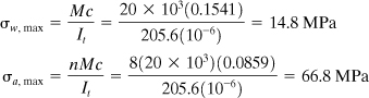
It is noted that at the juncture of the two parts:

b. For this case, the modular ratio n = E_w/E_a = 1/8 and the transformed area is shown in Fig. 5.13c. We now have

Then

as have already been found in part (a).

Example 5.5

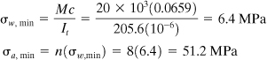
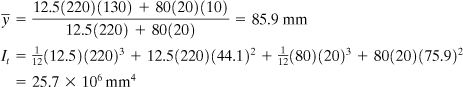
A concrete beam of width b = 250 mm and effective depth d = 400 mm is reinforced with three steel bars providing a total cross-sectional area A_s = 1000 mm² (Fig. 5.14a). Dimensions are given in millimeters. Note that it is usual for an approximate allowance a = 50 mm to be used to protect the steel from corrosion and fire. Let n = E_S/E_C = 10. Calculate the maximum stresses in the materials produced by a negative bending moment of M = 60 kN · m.

Figure 5.14. Example 5.5 Reinforced-concrete beam.

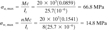
Solution Concrete is very weak in tension but strong in compression. Thus, only the portion of the cross section located a distance kd above the neutral axis is used in the transformed section (Fig. 5.14b); the concrete is assumed to take no tension. Notice that the transformed area of the steel nA_s is located by a single dimension from the neutral axis to its centroid. The compressive stress in the concrete is assumed to vary linearly from the neutral axis. The steel is taken to be uniformly stressed.

The condition that the first moment of the transformed section with respect to the neutral axis be zero is satisfied by

or

(5.54)

Solving this quadratic expression for kd, the position of the neutral axis is obtained.

Introducing the data given, Eq. (5.54) reduces to

(kd)² + 80(kd) − 32 × 10³ = 0

from which

(c)

The moment of inertia of the transformed cross section about the neutral axis is

Thus, the peak compressive stress in the concrete and the tensile stress in the steel are

The stresses act as shown in Fig. 5.14c.

An alternative method of solution is to obtain σ_{C, max} and σ_s from a free-body diagram of the portion of the beam (Fig. 5.14c) without computing I_t. The first equilibrium condition, ∑F_x = 0, gives C = T, where

(d)

are the compressive and tensile stress resultants, respectively. From the second requirement of statics, ∑M_Z = 0, we have

(e)

Equations (d) and (e) result in

(5.55)

Substitution of the data given and Eq. (c) into Eq. (5.55) yields

as before.

5.10. Shear Center

Given any cross-sectional configuration, one point may be found in the plane of the cross section through which passes the resultant of the transverse shearing stresses. A transverse load applied on the beam must act through this point, called the shear center or flexural center, if no twisting is to occur.^* The center of shear is sometimes defined as the point in the end section of a cantilever beam at which an applied load results in bending only. When the load does not act through the shear center, in addition to bending, a twisting action results (Sec. 6.1). The location of the shear center is independent of the direction and magnitude of the transverse forces. For singly symmetrical sections, the shear center lies on the axis of symmetry, while for a beam with two axes of symmetry, the shear center coincides with their point of intersection (also the centroid). It is not necessary, in general, for the shear center to lie on a principal axis, and it may be located outside the cross section of the beam.

^* For a detailed discussion, see Ref. 5.2.

For thin-walled sections, the shearing stresses are taken to be distributed uniformly over the thickness of the wall and directed so as to parallel the boundary of the cross section. If the shear center S for the typical section of Fig. 5.15a is required, we begin by calculating the shear stresses by means of Eq. (5.39). The moment M_x of these stresses about arbitrary point A is then obtained. Inasmuch as the external moment attributable to V_y about A is V_ye, the distance between A and the shear center is given by

(5.56)

Figure 5.15. Shear centers.

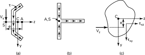
If the force is parallel to the z axis rather than the y axis, the position of the line of action may be established in the manner discussed previously. In the event that both V_y and V_z exist, the intersection of the two lines of action locates the shear center.

The determination of M_x is simplified by propitious selection of point A, such as in Fig. 5.15b. Here it is observed that the moment M_x of the shear forces about A is zero; point A is also the shear center. For all sections consisting of two intersecting rectangular elements, the same situation exists.

For the thin-walled box-beams (with boxlike cross section) the point or points in the wall where the shear flow q = 0 (or τ_xy = 0) is unknown. Here shear flow is represented by the superposition of transverse and torsional flow (see Sec. 6.7). Hence, the unit angle of twist equation, Eq. (6.23), along with q = VQ/I is required to find the shear flow for a cross section of a box beam. The analysis procedure is as follows: First introduce a free edge by cutting the section open; second close it again by obtaining the shear flow that makes the angle of twist in the beam zero [Refs. 5.3 through 5.5].

The preceding considerations can be extended to beams of arbitrary solid cross section, in which the shearing stress varies with both cross-sectional coordinates y and z. For these sections, the exact theory can, in some cases, be successfully applied to locate the shear center. Examine the section of Fig. 5.15c, subjected to the shear force V_z which produces the stresses indicated. Denote y and z as the principal directions. The moment about the x axis is

(5.57)

V_z must be located a distance e from the z axis, where e = M_x/V_Z.

In the following examples, the determination of the shear center of an open, thin-walled section is illustrated in the solution for two typical situations. The first refers to a section having only one axis of symmetry, the second to an asymmetrical section.

Example 5.6

Locate the shear center of the channel section loaded as a cantilever (Fig. 5.16a). Assume that the flange thicknesses are small when compared with the depth and width of the section.

Figure 5.16. Example 5.6.

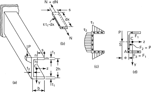
Solution The shearing stress in the upper flange at any section nn will be found first. This section is located a distance s from the free edge m, as shown in the figure. At m the shearing stress is zero. The first moment of area st₁ about the z axis is Q_z = st₁h. The shear stress at nn, from Eq. (5.39), is thus

(a)

The direction of τ along the flange can be determined from the equilibrium of the forces acting on an element of length dx and width s (Fig. 5.16b). Here the normal force N = t₁sσ_x, owing to the bending of the beam, increases with dx by dN. Hence, the x equilibrium of the element requires that τt₁ · dx must be directed as shown. As a consequence, this flange force is directed to the left, because the shear forces must intersect at the corner of the element.

The distribution of the shear stress τ_xz on the flange, as Eq. (a) indicates, is linear with s. Its maximum value occurs at s = b:

(b)

Similarly, the value of stress τ_xy at the top of the web is

(c)

The stress varies parabolically over the web, and its maximum value is found at the neutral axis. A sketch of the shear stress distribution in the channel is shown in Fig. 5.16c. As the shear stress is linearly distributed across the flange length, from Eq. (b), the flange force is expressed by

(d)

Symmetry of the section dictates that F₁ = F₃ (Fig. 5.16d). We shall assume that the web force F₂ = P, since the vertical shearing force transmitted by the flange is negligibly small, as shown in Example 5.3. The shearing force components acting in the section must be statically equivalent to the resultant shear load P. Thus, the principle of the moments for the system of forces in Fig. 5.16d or Eq. (5.56), applied at A, yields M_x = Pe = 2F₁h. Upon substituting F₁ from Eq. (d) into this expression, we obtain

where

The shear center is thus located by the expression

(e)

Note that e depends on only section dimensions. Examination reveals that e may vary from a minimum of zero to a maximum of b/2. A zero or near zero value of e corresponds to either a flangeless beam (b = 0, e = 0) or an especially deep beam (h >> b). The extreme case, e = b/2, is obtained for an infinitely wide beam.

Example 5.7

Locate the shear center center S for the asymmetrical channel section shown in Fig. 5.17a. All dimensions are in millimeters. Assume that the beam thickness t = 1.25 mm is constant.

Figure 5.17. Example 5.7.

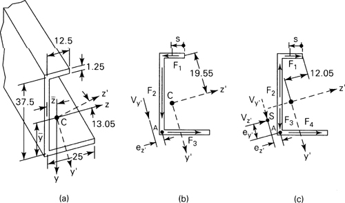
Solution The centroid C of the section is located by and with respect to nonprincipal axes z and y. By performing the procedure given in Example 5.1, we obtain = 15.63 mm, = 5.21 mm, I_y = 4765.62 mm⁴, I_z = 21,054.69 mm⁴, and I_yz = 3984.37 mm⁴. Equation (5.18) then yields the direction of the principal axis x′,y′ as θ_p = 13.05°, and Eq. (5.19), the principal moments of inertia I_y′ = 3828.12 mm⁴, I_z′ = 21,953.12 mm⁴ (Fig. 5.17a).

Let us now assume that a shear load V_y′ is applied in the y′, Z′ plane (Fig. 5.17b). This force may be considered the resultant of force components F₁, F₂, and F₃ acting in the flanges and web in the directions indicated in the figure. The algebra will be minimized if we choose point A, where F₂ and F₃ intersect, in finding the line of action of V_y′ by applying the principle of moments. In so doing, we need to determine the value of F₁ acting in the upper flange. The shear stress τ_XZ in this flange, from Eq. (5.39), is

(f)

where s is measured from right to left along the flange. Note that Q_Z′, the bracketed expression, is the first moment of the shaded flange element area with respect to the Z′ axis. The constant 19.55 is obtained from the geometry of the section. Upon substituting the numerical values and integrating Eq. (f), the total shear force in the upper flange is found to be

(g)

Application of the principle of moments at A gives V_y′e_Z′ = 37.5F₁. Introducing F₁ from Eq. (g) into this equation, the distance e_Z′, which locates the line of action of V_y′ from A, is

(h)

Next, assume that the shear loading V_Z′ acts on the beam (Fig. 5.17c). The distance e_y′ may be obtained as in the situation just described. Because of V_Z′, the force components F₁ to F₄ will be produced in the section. The shear stress in the upper flange is given by

(i)

Here Q_y′ represents the first moment of the flange segment area with respect to the y′ axis, and 12.05 is found from the geometry of the section. The total force F₁ in the flange is

The principle of moments applied at A, V_Z′e_y′ = 37.5F₁ = 7.65V_z′, leads to

(j)

Thus, the intersection of the lines of action of V_y′ and V_Z′, and e_Z′ and e_y′, locates the shear center S of the asymmetrical channel section.

5.11. Statically Indeterminate Systems

A large class of problems of considerable practical interest relates to structural systems for which the equations of statics are not sufficient (though necessary) for determination of the reactions or other unknown forces. Such systems are statically indeterminate, requiring supplementary information for solution. Additional equations usually describe certain geometrical conditions associated with displacement or strain. These equations of compatibility state that the strain owing to deflection or rotation must be such as to preserve continuity. With this additional information, the solution proceeds in essentially the same manner as for statically determinate systems. The number of reactions in excess of the number of equilibrium equations is called the degree of statical indeterminacy. Any reaction in excess of that which can be obtained by statics alone is said to be redundant. Thus, the number of redundants is the same as the degree of indeterminacy.

Several methods are available to analyze statically indeterminate structures. The principle of superposition, briefly discussed next, offers for many cases an effective approach. In Sec. 5.6 and in Chapters 7 and 10, a number of commonly employed methods are discussed for the solution of the indeterminate beam, frame, and truss problems.

The Method of Superposition

In the event of complicated load configurations, the method of superposition may be used to good advantage to simplify the analysis. Consider, for example, the continuous beam of Fig. 5.18a, replaced by the beams shown in Fig. 5.18b and c. At point A, the beam now experiences the deflections (ν_A)_p and (ν_A)_R due respectively to P and R. Subject to the restrictions imposed by small deformation theory and a material obeying Hooke’s law, the deflections and stresses are linear functions of transverse loadings, and superposition is valid:

υ_A = (υ_A)_p + (υ_A)_R

σ_A = (σ_A)_p + (σ_A)_R

Figure 5.18. Superposition of displacements in a continuous beam.

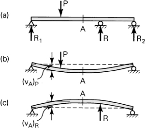
The procedure may in principle be extended to situations involving any degree of indeterminacy.

Example 5.8

A propped cantilever beam AB subject to a uniform load of intensity p is shown in Fig. 5.19. Determine (a) the reactions, (b) the equation of the deflection curve, and (c) the slope at A.

Figure 5.19. Example 5.8. Statically indeterminate beam.

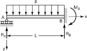
Solution Reactions R_A, R_B, and M_B are statically indeterminate because there are only two equilibrium conditions (Σ F_y = 0, Σ M_Z = 0); the beam is statically indeterminate to the first degree. With the origin of coordinates taken at the left support, the equation for the beam moment is

The third of Eqs. (5.32) then becomes

and successive integrations yield

(a)

There are three unknown quantities in these equations (c₁, c₂, and R_A) and three boundary conditions:

(b)

a. Introducing Eqs. (b) into the preceding expressions, we obtain c₂ = 0, c₁ = pL³/48, and

(5.58a)

We can now determine the remaining reactions from the equations of equilibrium:

(5.58b,c)

b. Substituting for R_A, c₁ and c₂ in Eq. (a), the equation of the deflection curve is obtained:

(5.59)

c. Differentiating the foregoing with respect to x, the equation of the angle of rotation is

(5.60)

Setting x = 0, we have the slope at A:

(5.61)

Example 5.9

Consider again the statically indeterminate beam of Fig. 5.19. Determine the reactions using the method of superposition.

Solution Reaction R_A is selected as redundant and is considered an unknown load by eliminating the support at A (Fig. 5.20a). The loading is resolved into those shown in Fig. 5.20b. The solution for each case is (see Table D.4)

Figure 5.20. Example 5.9.

The compatibility condition for the original beam requires that

from which R_A = 3pL/8. Reaction R_B and moment M_B can now be found from the equilibrium requirements. The results correspond to those of Example 5.8.

5.12. Energy Method for Deflections

Strain energy methods are frequently employed to analyze the deflections of beams and other structural elements. Of the many approaches available, Castigliano’s second theorem is one of the most widely used. In applying this theory, the strain energy must be represented as a function of loading. Detailed discussions of energy techniques are found in Chapter 10. In this section we limit ourselves to a simple example to illustrate how the strain energy in a beam is evaluated and how the deflection is obtained by the use of Castigliano’s theorem (Sec. 10.4).

The strain energy stored in a beam under bending stress σ_x only, substituting M = EI(d²υ/dx²) into Eq. (2.53), is expressed in the form

(5.62)

Here the integrations are carried out over the beam length. We next determine the strain energy stored in a beam, only due to the shear loading V. As we described in Sec. 5.7, this force produces shear stress τ_xy at every point in the beam. The strain energy density is, from Eq. (2.40), . Substituting τ_xy as expressed by Eq. (5.39), we have U_º = V²Q²/2GI²b². Integrating this expression over the volume of the beam of cross-sectional area A, we obtain

(a)

Let us denote

(5.63)

This is termed the form factor for shear, which when substituted in Eq. (a) yields

(5.64)

where the integration is carried over the beam length.

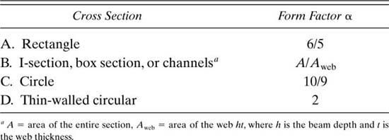
The form factor is a dimensionless quantity specific to a given cross-section geometry. For example, for a rectangular cross section of width b and height 2h, the first moment Q, from Eq. (5.41), is . Because A/I² = 9/2bh⁵, Eq. (5.63) provides the following result:

(b)

In a like manner, the form factor for other cross sections can be determined. Table 5.1 lists several typical cases. Following the determination of α, the strain energy is evaluated by applying Eq. (5.64).

Table 5.1. Form Factor for Shear for Various Beam Cross Sections

For a linearly elastic beam, Castigliano’s theorem, from Eq. (10.3), is expressed by

(c)

where P is a load acting on the beam and δ is the displacement of the point of application in the direction of P. Note that the strain energy U = U_b + U_s is expressed as a function of the externally applied forces (or moments).

As an illustration, consider the bending of a cantilever beam of rectangular cross section and length L, subjected to a concentrated force P at the free end (Fig. 5.5). The bending moment at any section is M = Px, and the shear force V is equal in magnitude to P. Upon substituting these together with into Eqs. (5.62) and (5.64) and integrating, the strain energy stored in the cantilever is found to be

The displacement of the free end owing to bending and shear is, by application of Castigliano’s theorem, therefore

The exact solution is given by Eq. (5.24).

Part C—Curved Beams

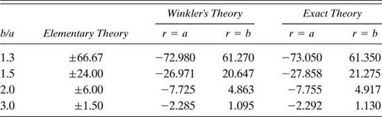
5.13. Exact Solution

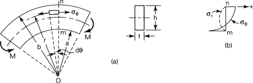
A curved bar or beam is a structural element for which the locus of the centroids of the cross sections is a curved line. This section concerns itself with an application of the theory of elasticity. We deal here with a bar characterized by a constant narrow rectangular cross section and a circular axis. The axis of symmetry of the cross section lies in a single plane throughout the length of the member.

Consider a beam subjected to equal end couples M such that bending takes place in the plane of curvature, as shown in Fig. 5.21a. Inasmuch as the bending moment is constant along the length of the bar, the stress distribution should be identical in any radial cross section. Stated differently, we seek a distribution of stress displaying θ independence. It is clear that the appropriate expression of equilibrium is Eq. (8.2),

(a)

Figure 5.21. Pure bending of a curved beam of rectangular cross section.

and that the condition of compatibility for plane stress, Eq. (3.38),

must also be satisfied. The latter is an equidimensional equation, reducible to a second-order equation with constant coefficients by substituting r = e^t or t = In r. Direct integration then leads to σ_r + σ_θ = c" + c′ In r, which may be written in the form σ_r + σ_θ = c″ + c′ In(r/a). Solving this expression together with Eq. (a) results in the following equations for the radial and tangential stress:

(5.65)

To evaluate the constants of integration, the boundary conditions are applied as follows:

1. No normal forces act along the curved boundaries at r = a and r = b, and therefore

(b)

2. Because there is no force acting at the ends, the normal stresses acting at the straight edges of the bar must be distributed to yield a zero resultant:

(c)

where t represents the beam thickness.

3. The normal stresses at the ends must produce a couple M:

(d)

The conditions (c) and (d) apply not only at the ends, but because of σ_θ independence, at any θ. In addition, shearing stresses have been assumed zero throughout the beam, and τ_rθ = 0 is thus satisfied at the boundaries, where no tangential forces exist.

Combining the first equation of (5.65) with the conditions (b), we find that

These constants together with the second of Eqs. (5.65) satisfy condition (c). Thus, we have

(e)

Finally, substitution of the second of Eqs. (5.65) and (e) into (d) provides

(f)

where

(5.66)

When the expressions for constants c₁, c₂, and c₃ are inserted into Eq. (5.65), the following equations are obtained for the radial and tangential stress:

(5.67)

If the end moments are applied so that the force couples producing them are distributed in the manner indicated by Eq. (5.67), then these equations are applicable throughout the bar. If the distribution of applied stress (to produce M) differs from Eq. (5.67), the results may be regarded as valid in regions away from the ends, in accordance with Saint-Venant’s principle. The foregoing results, when applied to a beam with radius a, large relative to its depth h, yield an interesting comparison between straight and curved beam theory. For h << a, σ_r in Eq. (5.67) becomes negligible, and σ_θ is approximately the same as that obtained from My/I.

The bending moment is taken as positive when it tends to decrease the radius of curvature of the beam, as in Fig. 5.21a. Employing this sign convention, σ_r as determined from Eq. (5.67) is always negative, indicating that it is compressive. Similarly, when σ_θ is found to be positive, it is tensile; otherwise, compressive. In Fig. 5.21b, a plot of the stresses at section mn is presented. Note that the maximum stress magnitude is found at the extreme fiber of the concave side.

Deflections

Substitution of σ_r and σ_θ from Eq. (5.67) into Hooke’s law provides expressions for the strains ε_θ, ε_r, and γ_rθ. The displacements u and ν then follow, upon integration, from the strain–displacement relationships, Eqs. (3.30). The resulting displacements indicate that plane sections of the curved beam subjected to pure bending remain plane subsequent to bending. Castigliano’s theorem (Sec. 5.12) is particularly attractive for determining the deflection of curved members.

For beams in which the depth of the member is small relative to the radius of curvature or, as is usually assumed, R/c > 4, the initial curvature may be neglected in evaluating the strain energy. Here R represents the radius to the centroid, and c is the distance from the centroid to the extreme fiber on the concave side. Thus, the strain energy due to the bending of a straight beam [Eq. (5.62)] is a good approximation also for curved, slender beams.

5.14. Tangential Stress. Winkler’s Theory

The approach to curved beams now explored is due to E. Winkler. As an extension of the elementary theory of straight beams, in Winkler’s theory it will be assumed that all conditions required to make the straight-beam formula applicable are satisfied except that the beam is initially curved. Consider the pure bending of a curved beam as in Fig. 5.22a. The distance from the center of curvature to the centroidal axis is R. Derivation of the stress in the beam is again based on the three principles of solid mechanics and the familiar assumptions:

Figure 5.22. Curved beam in pure bending with a cross-sectional axis of symmetry.

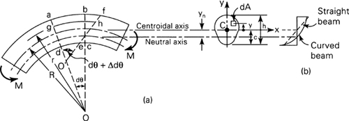
1. All cross sections possess a vertical axis of symmetry lying in the plane of the centroidal axis passing through C.

2. The beam is subjected to end couples M. The bending moment vector is every where normal to the plane of symmetry of the beam.

3. Sections originally plane and perpendicular to the centroidal beam axis remain so subsequent to bending. (The influence of transverse shear on beam deformation is not taken into account.)

Referring to assumption (3), note the relationship in Fig. 5.22a between lines bc and ef representing plane sections before and after the bending of an initially curved beam. Note also that the initial length of a beam fiber such as gh depends on the distance r from the center of curvature O. On the basis of plane sections remaining plane, we can state that the total deformation of a beam fiber obeys a linear law, as the beam element rotates through small angle Δ dθ. The tangential strain ε_θ does not follow a linear relationship, however. The deformation of arbitrary fiber gh is ε_cR dθ + yΔ dθ, where ε_c denotes the strain of the centroidal fiber. Since the original length of gh is (R + y) dθ, the tangential strain of this fiber is given by ε_θ = (ε_c R dθ + y Δ dθ)/(R + y) dθ. Through introduction of Hooke’s law, the tangential stress acting on area dA is then

Denoting the angular strain Δ dθ/dθ by λ and adding and subtracting ε_c y in the numerator, we put the preceding expression into a more convenient form:

(a)

The beam section must, of course, satisfy the conditions of static equilibrium, F_Z = 0 and M_x = 0, respectively:

(b)

When the tangential stress of Eq. (a) is inserted into Eq. (b), we obtain

(c)

Note the ƒ dA = A, and since y is measured from the centroidal axis, ƒ ydA = 0.

We now introduce the notation for a property of the area, the curved beam factor:

(5.68)

It follows that

(d)

Equations (c) are thus written ε_c = (λ – ε_c)Z and M = E(λ – ε_c) · ZAR. From these.

(e)

Substitution of Eqs. (e) into Eq. (a) provides an expression for the tangential stress in a curved beam subject to pure bending:

(5.69)

This equation is often referred to as Winkler’s formula. The variation of stress over the cross section is hyperbolic, as sketched in Fig. 5.22b. The sign convention applied to bending moment is the same as that used in Sec. 5.13. The bending moment is positive when directed toward the concave side of the beam, as shown in the figure. If Eq. (5.69) results in a positive value, it is indicative of a tensile stress.

The distance between the centroidal axis (y = 0) and the neutral axis is found by setting equal to zero the tangential stress in Eq. (5.69):

(f)

where y_n denotes the distance between axes, as indicated in Fig. 5.22a. From this,

(5.70)

This expression is valid for the case of pure bending only.

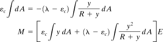
Comparison of the results of the various theories. To do this, consider a curved beam of rectangular cross section and unit thickness experiencing pure bending. The tangential stress predicted by the elementary theory (based on a linear distribution of stress) is My/I. The Winkler approach, leading to a hyperbolic distribution, is given by Eq. (5.69), while the exact theory results in Eqs. (5.67). In each case, the maximum and minimum values of stress are expressible by

(5.71)

In Table 5.2, values of m are listed as a function of b/a for the four cases cited [Ref. 5.6]. Observe that there is good agreement between the exact and Winkler results. On this basis as well as from more extensive comparisons, it may be concluded that the Winkler approach is adequate for practical applications. Its advantage lies in the relative ease with which it may be applied to any symmetric section.

Table 5.2.

The agreement between the Winkler and exact analyses is not as good in situations of combined loading as for the case of pure bending. As might be expected, for beams of only slight curvature, the simple flexure formula provides good results while requiring only simple computation. The linear and hyperbolic stress distributions are approximately the same for R/c > 20.

Finally, it is noted that where I-, T-, or thin-walled tubular curved beams are involved, the stresses predicted by the approaches developed in this chapter will be in error. This is attributable to high stresses existing in certain sections such as the flanges, which cause significant beam distortion. A modified Winkler’s equation finds application in such situations if more accurate results are required [Ref. 5.7].

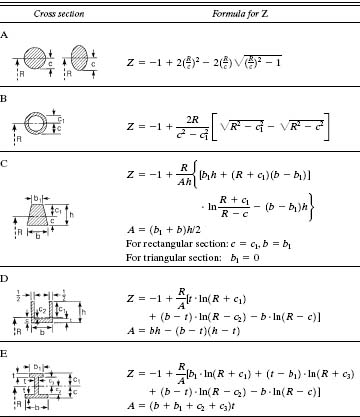
To illustrate the derivation of the curved beam factor, let us consider a circular frame of inner radius a (Fig. 5.23a). The rectangular cross section has a width h and thickness t, as shown in Fig. 5.23b. Applying Eq. (5.68) with c_A = c_B = c, we write

(g)

Figure 5.23. Curved beam with rectangular cross section.

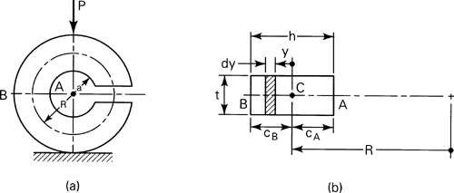
This expression may in general be evaluated through direct integration by use of the binomial expansion and integration or by numerical techniques. Through direct integration, Eq. (g) yields

(h)

Alternatively, expanding in a binomial series,

Substituting this expression in Eq. (g), we have

(i)

Employing similar methods, expressions for the curved beam factor Z for other sections may be found. Table 5.3 lists some commonly encountered examples.

Table 5.3.

5.15. Combined Tangential and Normal Stresses

The tangential stress given by Eq. (5.69) may be added to the stress produced by a normal load P acting through the centroid of cross-sectional area A. For this simple case of superposition,

(5.72)

As before, a negative sign would be associated with a compressive load P.

Example 5.10

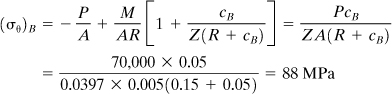
A load P of 70 kN is applied to the circular steel frame shown in Fig. 5.23a. Dimensions are a = 100 mm, h = 100 mm, and t = 50 mm. Determine the tangential stress at points A and B.

Solution From Eq. (h) with R = 0.1 + 0.05 = 0.15 m and c_A = c_B = C 0.05 m (Fig. 5.23b), it is found that

The stresses at the inner and outer edges of section A-B, with M = PR, are thus

(5.73)

(5.74)

Example 5.11

A steel ring of 350-mm mean diameter and of uniform rectangular section 60 mm wide and 12 mm thick is shown in Fig. 5.24a. A rigid bar is fitted across diameter AB, and a tensile force P applied to the ring as shown. Assuming an allowable stress of 140 MPa, determine the maximum tensile force that can be carried by the ring.

Figure 5.24. Example 5.11

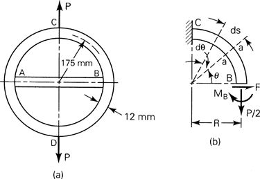
Solution Let the thrust induced in bar AB be denoted by 2F. The moment at any section a-a (Fig. 5.24b) is then

(a)

Note that before and after deformation the relative slope between B and C remains unchanged. Therefore, the relative angular rotation between B and C is zero. Applying Eq. (5.32), we therefore obtain

where dx = ds = R dθ is the length of beam segment corresponding to dθ. Upon substitution of Eq. (a), this becomes, after integrating,

(b)

This expression involves two unknowns, M_B and F. Another expression in terms of M_B and F is found by recognizing that the deflection at B is zero. By application of Castigliano’s theorem,

where U is the strain energy of the segment. This expression, upon introduction of Eq. (a), takes the form

After integration,

(c)

Solution of Eqs. (b) and (c) yields M_B = 0.1106PR and FR = 0.4591PR. Substituting Eq. (a) gives, for θ = 90°,

Thus, M_c > M_B. Since R/c = 0.175/0.006 = 29, the simple flexure formula offers the most efficient means of computation. The maximum stress is found at points A and B:

Similarly, at C and D,

Hence σ_θC > σ_θB. Since σ_max = 140 MPa, 140 × 10⁶ = 18,411P. The maximum tensile load is therefore P = 7.604 kN.

Problems

Secs. 5.1 through 5.5

5.1. A simply supported beam constructed of a 0.15 × 0.15 × 0.015 m angle is loaded by concentrated force P = 22.5 kN at its midspan (Fig. P5.1). Calculate stress σ_x at A and the orientation of the neutral axis. Neglect the effect of shear in bending and assume that beam twisting is prevented.

Figure P5.1.

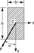
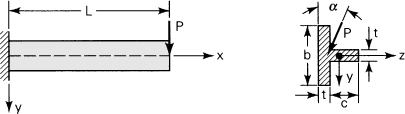
5.2. A wood cantilever beam with cross section as shown in Fig. P5.2 is subjected to an inclined load P at its free end. Determine (a) the orientation of the neutral axis; (b) the maximum bending stress. Given data: P = 1 kN, α = 30°, b = 80 mm, h = 150 mm, and length L = 1.2 m.

Figure P5.2.

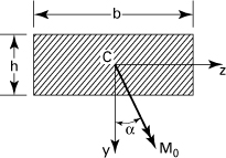
5.3. A moment M_o is applied to a beam of the cross section shown in Fig. P5.3 with its vector forming an angle of α. Use b = 100 mm, h = 40 mm, M_o = 800 N · m, and α = 25°. Calculate (a) the orientation of the neutral axis; (b) the maximum bending stress.

Figure P5.3.

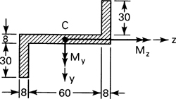
5.4. Couples M_y = M_o and M_z = 1.5M_o are applied to a beam of cross section shown in Fig. P5.4. Determine the largest allowable value of M_o, for the maximum stress not to exceed 80 MPa. All dimensions are in millimeters.

Figure P5.4.

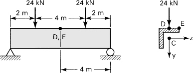
5.5. For the simply supported beam of Fig. P5.5, determine the bending stress at points D and E. The cross section is a 0.15 × 0.15 × 0.02 m angle (Fig. 5.4).

Figure P5.5.

5.6. A concentrated load P acts on a cantilever as shown in Fig. P5.6. The beam is constructed of a 2024-T4 aluminum alloy having a yield strength σ_yp = 290 MPa, L = 1.5 m, t = 20 mm, c = 60 mm, and b = 80 mm. Based on a factor of safety n = 1.2 against initiation of yielding, calculate the magnitude of P for (a) α = 0° and (b) α = 15°. Neglect the effect of shear in bending and assume that beam twisting is prevented.

Figure P5.6.

5.7. Redo Prob. 5.6 for α = 30°. Assume the remaining data to be unchanged.

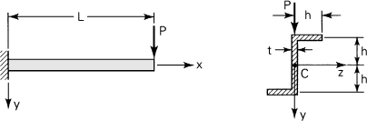
5.8. A cantilever beam has a Z section of uniform thickness for which , , and I_yz = –th³. Determine the maximum bending stress in the beam subjected to a load P at its free end (Fig. P5.8).

Figure P5.8.

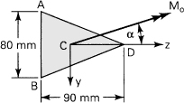
5.9. A beam with cross section as shown in Fig. P5.9 is acted on by a moment M₀= 3 kN · m with its vector forming an angle α = 20°. Determine (a) the orientation of the neutral axis, and (b) the maximum bending stress.

Figure P5.9.

5.10. For the thin cantilever of Fig. P5.10, the stress function is given by

a. Determine the stresses σ_x, σ_y, and τ_xy by using the elasticity method.

b. Determine the stress σ_x by using the elementary method.

Figure P5.10.

c. Compare the values of maximum stress obtained by the preceding approaches for L = 10h.

5.11. Consider a cantilever beam of constant unit thickness subjected to a uniform load of p = 2000 kN per unit length (Fig. P5.11). Determine the maximum stress in the beam:

Figure P5.11.

a. Based on a stress function

b. Based on the elementary theory. Compare the results of (a) and (b).

Secs. 5.6 through 5.11

5.12. A bending moment acting about the z axis is applied to a T-beam shown in Fig. P5.12. Take the thickness t = 15 mm and depth h = 90 mm. Determine the width b of the flange in order that the stresses at the bottom and top of the beam will be in the ratio 3 : 1, respectively.

Figure P5.12.

5.13. A wooden, simply supported beam of length L is subjected to a uniform load p. Determine the beam length and the loading necessary to develop simultaneously σ_max = 8.4 MPa and τ_max = 0.7 MPa. Take thickness t = 0.05 m and depth h = 0.15 m.

5.14. A box beam supports the loading shown in Fig. P5.14. Determine the maximum value of P such that a flexural stress σ = 7 MPa or a shearing stress τ = 0.7 MPa will not be exceeded.

Figure P5.14.

5.15. A composite cantilever beam 140 mm wide, 300 mm deep, and 3 m long is fabricated by fastening two timber planks (E_t = 10 GPa), 60 mm × 300 mm, to the sides of a steel plate (E_s = 200 GPa), 20 mm wide by 300 mm deep. Note that the 300-mm dimension is vertical. The allowable stresses in bending for timber and steel are 7 and 120 MPa, respectively. Calculate the maximum vertical load P the beam can carry at its free end.

5.16. A 180-mm-wide by 300-mm-deep wood beam (E_w = 10 GPa) 4 m long is reinforced with 180-mm-wide and 10-mm-deep aluminum plates (E_a = 70 GPa) on the top and bottom faces. The beam is simply supported and subject to a uniform load of intensity 25 kN/m over its entire length. Calculate the maximum stresses in each material.

5.17. Referring to the reinforced concrete beam of Fig. 5.14a, b = 300 mm, d = 450 mm, A_s = 1200 mm², and n = 10. Given allowable stresses in steel and concrete of 150 and 12 MPa, respectively, calculate the maximum bending moment the section can carry.

5.18. Referring to the reinforced concrete beam of Fig. 5.14a, b = 300 mm, d = 500 mm, and n = 8. Given the actual maximum stresses developed to be σ_s = 80 MPa and σ_c = 5 MPa, calculate the applied bending moment and the steel area required.

5.19. A beam is constructed of half a hollow tube of mean radius R and wall thickness t (Fig. P5.19). Assuming t << R, locate the shear center S. The moment of inertia of the section about the z axis is I_z = πR³t/2.

Figure P5.19.

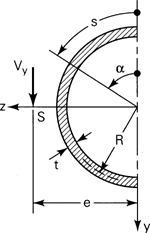
5.20. An H-section beam with unequal flanges is subjected to a vertical load P (Fig. P5.20). The following assumptions are applicable:

Figure P5.20.

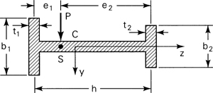
1. The total resisting shear occurs in the flanges.

2. The rotation of a plane section during bending occurs about the symmetry axis so that the radii of curvature of both flanges are equal.

Determine the location of the shear center S.

5.21. Determine the shear center S of the section shown in Fig. P5.21. All dimensions are in millimeters.

Figure P5.21.

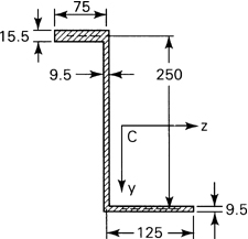
5.22. A cantilever beam AB supports a triangularly distributed load of maximum intensity p₀ (Fig. P5.22). Determine (a) the equation of the deflection curve, (b) the deflection at the free end, and (c) the slope at the free end.

Figure P5.22.

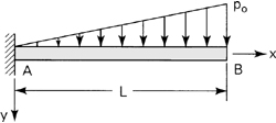
5.23. The slope at the wall of a built-in beam (Fig. P5.23a) is as shown in Fig. P5.23b and is given by pL³/96EI. Determine the force acting at the simple support, expressed in terms of p and L.

5.24. A fixed-ended beam of length L is subjected to a concentrated force P at a distance c away from the left end. Derive the equations of the elastic curve.

Figure P5.23.

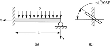
5.25. A propped cantilever beam AB is subjected to a couple M₀ acting at support B, as shown in Fig. P5.25. Derive the equation of the deflection curve and determine the reaction at the roller support.

Figure P5.25.

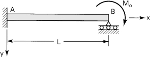
5.26. A welded bimetallic strip (Fig. P5.26) is initially straight. A temperature increment ΔT causes the element to curve. The coefficients of thermal expansion of the constituent metals are α₁ and α₂. Assuming elastic deformation and α₂ > α₁, determine (a) the radius of curvature to which the strip bends, (b) the maximum stress occurring at the interface, and (c) the temperature increase that would result in the simultaneous yielding of both elements.

Figure P5.26.

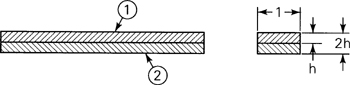
Secs. 5.12 through 5.15

5.27. Verify the values of α for cases B, C, and D of Table 5.1.

5.28. Consider a curved bar subjected to pure bending (Fig. 5.21). Assume the stress function

Φ = A In r + Br² In r + Cr² + D

to rederive the stress field in the bar given by Eqs. (5.67).

5.29. The cross section of a curved beam is shown in Fig. P5.29. Derive the curved beam factor Z by means of integration. Compare the result with that given for Fig. D in Table 5.3.

Figure P5.29.

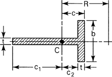
5.30. Verify the value of Z in Fig. B of Table 5.3.

5.31. The circular steel frame of Fig. 5.23 has a cross section approximated by the trapezoidal form shown in Fig. C of Table 5.3. What is the maximum load P for which the stress will not exceed 120 MPa? Take b = 0.1 m, b₁ = 0.06 m, and h = 0.12 m.

5.32. For the hook of circular cross section shown in Fig. P5.32, determine (a) the maximum load P that may be supported without exceeding a stress of 161 MPa at point A and (b) the tangential stress at point B of section A–B for the load obtained in (a).

Figure P5.32.

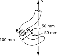
5.33. Determine the maximum tangential stress in the frame shown in Fig. 5.23, using the second of Eqs. (5.67) together with the method of superposition. Compare the value obtained with that found in Example 5.10.

5.34. The allowable stress in tension and compression for the clamp body shown in Fig. P5.34 is 80 MPa. Calculate the maximum permissible load the member can resist. Dimensions are in millimeters.

Figure P5.34.

5.35. A machine component of channel cross-sectional area is loaded as shown in Fig. P5.35. Calculate the tangential stress at points A and B. All dimensions are in millimeters.

Figure P5.35.

5.36. A load P is applied to an eye bar with rigid insert for the purpose of pulling (Fig. P5.36). Determine the tangential stress at points A and B (a) by the elasticity theory, (b) by Winkler’s theory, and (c) by the elementary theory. Compare the results obtained.

Figure P5.36.

5.37. A ring of mean radius R and constant rectangular section is subjected to a concentrated load (Fig. P5.37). You may omit the effect of shear in bending. Derive the following general expression for the tangential stress at any section of the ring:

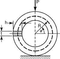
(P5.37)

where

Use Castigliano’s theorem.

Figure P5.37.

5.38. The ring shown in Fig. P5.37 has the following dimensions: R = 150 mm, t = 50 mm, and h = 100 mm. Taking , determine (a) the tangential stress on the inner fiber at θ = π/4 and (b) the deflection along the line of action of the load P, considering the effects of the normal and shear forces, as well as bending moment (Sec. 10.4).