
Chapter 6. Exact Calculation Procedures for Multicomponent Distillation
Since multicomponent calculations are trial and error, it is convenient to do them on a computer. Because stage-by-stage calculations are restricted to problems in which an accurate first guess of compositions can be made at some point in the column, matrix methods for multicomponent distillation are commonly used because these methods do not require a good guess of compositions.
6.0 Summary—Objectives
In this chapter we develop matrix methods for multicomponent distillation. When finished studying this chapter, you should be able to satisfy the following objectives:
1. Use a matrix approach to solve the multicomponent mass balances
2. Use bubble-point calculations to determine new temperatures on each stage
3. Use a matrix approach to solve the energy balances for new flow rates.
4. Explain the difference between the bubble-point and Naphtali-Sandholm methods
5. Use a process simulator to simulate multicomponent distillation
6.1 Introduction to Matrix Solution for Multicomponent Distillation
Since distillation is a very important separation technique, considerable effort has been spent in devising better calculation procedures. Details of these procedures are available in a variety of textbooks (Seader et al., 2011; Holland, 1981; King, 1981; Smith, 1963; and Wankat, 1988).
The general behavior of multicomponent distillation columns (see Chapter 5) and the basic mass and energy balances and equilibrium relationships do not change when different calculation procedures are used. (The physical operation is unchanged; thus, the basic laws and the results are invariant.) What different calculation procedures do is rearrange the equations to enhance convergence, particularly when it is difficult to make a good first guess. The most common approach is to group and solve the equations by type, not stage by stage. That is, all mass balances for component i are grouped and solved simultaneously, all energy balances are grouped and solved simultaneously, and so forth. Most of the equations can conveniently be written in matrix form. Computer routines for solution of these equations are easily written. The advantage of this approach is that even very difficult problems can be made to converge.
A convenient set of variables to specify is F, zi, TF, N, NF, p, Treflux, L/D, and D. Multiple feeds can be specified. This approach then becomes a simulation problem with the distillate flow rate specified. Because the matrices require that N and NF be known, for design problems, a good first guess of N and NF must be made (see Chapter 7) and then a series of simulation problems are solved to find the best design.
In Section 2.7 we looked at solution methods for multicomponent flash distillation. The questions asked in that section are again pertinent for multicomponent distillation. First, what trial variables should we use? As noted, because N and NF are required to set up the matrices, in design problems we choose these and solve a number of simulation problems to find the best design. We select the temperature on every stage, Tj, because temperature is needed to calculate K values and enthalpies. We also estimate the overall liquid, Lj, and vapor, Vj, flow rates on every stage because these flow rates are needed to solve the component mass balances.
Next, we need to decide if we should converge on all the trial variables in a sequential or simultaneous fashion. Since commercial simulators often allow the user to select either of these approaches, we consider both sequential and simultaneous approaches. The simultaneous approach is discussed in Section 6.6.
If we decide to use a sequential approach, we must decide which trial variable to converge on first: temperatures or flow rates. The answer depends on the type of problem we wish to solve. Distillation problems, which tend to be narrow boiling, usually converge best if temperature is converged on first. This method is illustrated in this chapter. Wide-boiling feeds such as flash distillation (Section 2.7), petroleum fractionation, and absorption and stripping (Chapter 12) tend to converge best if the sum-rates method (Section 12.9) that converges on flow rates first is used.
The narrow-boiling, or bubble-point, procedure used for distillation is shown in Figure 6-1. This procedure uses the equilibrium (bubble-point) calculations to determine new temperatures. The energy balance is used to calculate new flow rates. Temperatures are calculated and converged on first and then new flow rates are determined. This procedure makes sense, since an accurate first guess of liquid and vapor flow rates can be made by assuming constant molal overflow (CMO). Thus, temperatures are calculated using reasonable flow rate values. The energy balances are used last because they require values for xi,j, yi,j, and Tj.
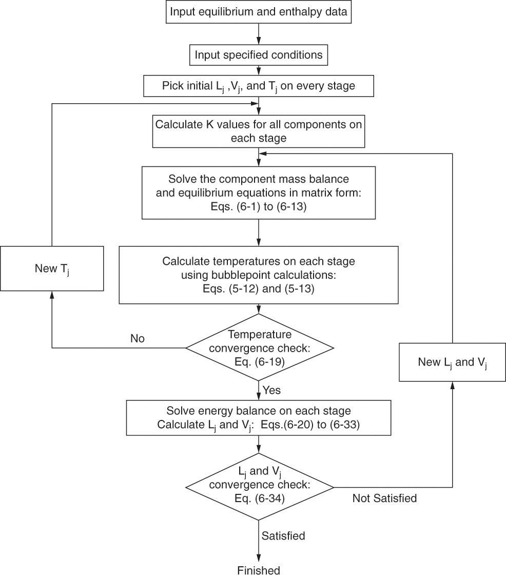
Figure 6-1 is constructed for an ideal system in which the Ki values depend only on temperature and pressure. If the Ki values depend on compositions, then compositions must be guessed and corrected before doing the temperature calculation. We discuss only systems in which Ki = Ki(T, p).
6.2 Component Mass Balances in Matrix Form
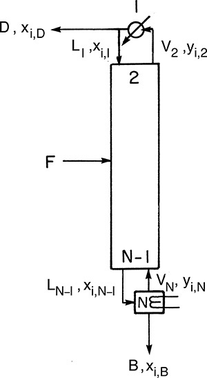
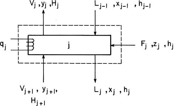
Amundson and Pontinen (1958) realized that the component mass balance equations for multicomponent distillation can be put into matrix form with one matrix for each component. To conveniently put the mass balances in matrix form, renumber the column as shown in Figure 6-2. Stage 1 is the total condenser, stage 2 is the top stage in the column, stage N-1 is the bottom stage, and the partial reboiler is listed as N. For a general stage j within the column (Figure 6-3), the mass balance for any component i is
The unknown vapor compositions, yi,j and yi,j+1, can be replaced using the equilibrium expressions
where the K values depend on T and p. If we also replace xi,j and xi,j–1 with
where ![]() ij and
ij and ![]() ij-1 are the liquid component flow rates, we obtain
ij-1 are the liquid component flow rates, we obtain
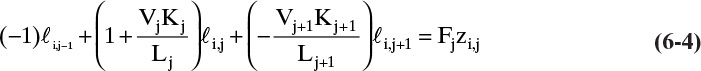
For each component, this equation can be written in the general form
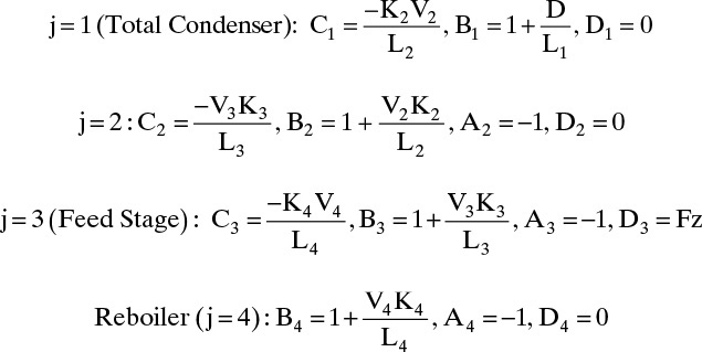
The constants Aj, Bj, Cj, and Dj are determined by comparing Eqs. (6-4) and (6-5).

Equations (6-4) and (6-5) are valid for all stages in the column, 2 ≤ j ≤ N – 1, and are repeated for each of the C components. If a stage has no feed, then Fj = Dj = 0.
For a total condenser, the mass balance is
Since x1 = xD, y2 = K2x2 and x1 = ![]() /L1 this equation becomes
/L1 this equation becomes
where
Note that only B1 does not follow the general formulas of Eq. (6-6). This occurs because the total condenser is not an equilibrium contact.
For the partial reboiler, the mass balance is
Substituting yN = KNxN and ![]() N = LNxN = Bxbot, we get
N = LNxN = Bxbot, we get
where

In matrix notation, the component mass balance and equilibrium relationship for each component is
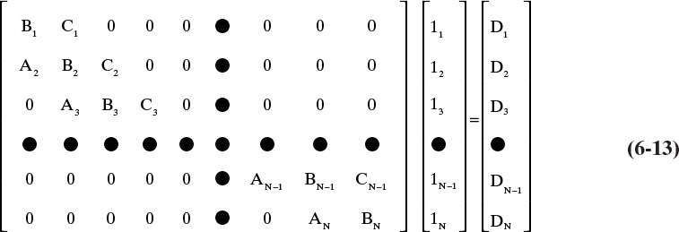
This set of simultaneous linear algebraic equations can be solved by inverting the ABC matrix. This can be done using any standard matrix inversion routine. The particular matrix form shown in Eq. (6-13) is a tridiagonal matrix, which is particularly easy to invert using the Thomas algorithm (see Table 6-1) (Lapidus, 1962; King, 1981). Inversion of the ABC matrix allows direct determination of the component liquid flow rate, lj, leaving each contact. You must construct the ABC matrix and invert it for each of the components.
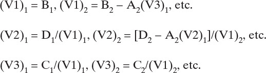
Consider the solution of a matrix in the form of Eq. (6-13) where all Aj, Bj, Cj, and Dj are known.
1. Calculate three intermediate variables for each row of the matrix starting with j = 1. For 1 ≤ j ≤ N,
(V1)j = Bj – Aj(V3)j–1
(V2)j = [Dj – Aj(V2)j–1]/(V1)j
(V3)j = Cj/(V1)j
since A1 ≡ 0, (V1)1 = B1, and (V2)1 = D1/(V1)1.
2. Initialize (V3)0 = 0 and (V2)0 = 0 so you can use the general formulas.
3. Calculate all unknowns, Uj [![]() i,j in Eq. (6-13), Vj in Eq. (6-28), or ΔTj in Eq. (12-58)]. Start with j = N, and calculate UN = (V2)N
i,j in Eq. (6-13), Vj in Eq. (6-28), or ΔTj in Eq. (12-58)]. Start with j = N, and calculate UN = (V2)N
Then going from j = N – 1 to j = 1, calculate UN–1, UN–2, ... U1 from Uj = (V2)j – (V3)jUj+1, 1 ≤ j ≤ N–1
TABLE 6-1. Thomas algorithm for inverting tridiagonal matrices
The A, B, and C terms in Eq. (6-13) must be calculated, but they depend on the liquid and vapor flow rates and the temperature (in the K values) on each stage, which we do not know. To start, guess Lj, Vj, and Tj for every stage j! For ideal systems the K values can be calculated for each component on every stage. Then the A, B, and C terms can be calculated for each component on every stage. Inversion of the matrices for each component gives all liquid component flow rates, ![]() i,j. These flow rates are correct for the assumed Lj, Vj, and Tj.
i,j. These flow rates are correct for the assumed Lj, Vj, and Tj.
6.3 Initial Guesses for Flow Rates and Temperatures
A reasonable first guess for Lj and Vj is to assume CMO. CMO was not assumed in Eqs. (6-1) to (6-13). With the CMO assumption, we can use overall mass balances to calculate all Lj and Vj.
To start the calculation we need to assume the split for non-key (NK) components. Usually the first assumption is that all the light non-key (LNK) components exit in the distillate so that xLNK,bot = 0 and DxLNK,dist = FzLNK. And all heavy non-key (HNK) components exit in the bottoms, xHNK,dist = 0 and BxHNK,bot = FzHNK. Next we do external mass balances to find all distillate and bottoms compositions and flow rates. This procedure is illustrated in Chapter 5. Once this is done, we can find L and V in the rectifying section. Since CMO is assumed,
At the feed stage, q can be estimated from enthalpies as

or q = LF/F can be found from a flash calculation on the feed stream. Then ![]() and
and ![]() are determined from balances at the feed stage:
are determined from balances at the feed stage:
This completes the preliminary calculations for flow rates.
We can estimate the temperature from bubble-point calculations (Section 5.3). Often it is sufficient to do a bubble-point calculation for the feed and then use this temperature on every stage. A better first guess can be obtained by estimating the distillate and bottoms compositions (usually NKs do not distribute), doing bubble-point calculations for both, and assuming that the temperature varies linearly from stage to stage.
6.4 Temperature Convergence
After the first guess and the solution of the matrix equations, the temperature must be corrected. This is done with bubble-point calculations on each stage.
Now the component flow rates are used to determine the liquid mole fractions.
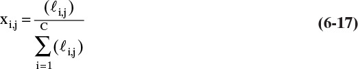
This procedure normalizes the mole fractions on each stage so that they sum to 1.0. Once the mole fractions have been determined, the new temperatures on each stage are calculated with bubble-point calculations (Section 5.3), which are illustrated in Example 6-1. To prevent excessive oscillation of temperatures, the change in temperature can be damped:
where df is a damping factor. When df = 1.0, this procedure becomes direct substitution.
The new temperatures are used to calculate the new K values (see Figure 6-1) and then the new A, B, and C coefficients for Eq. (6-13). The component mass balance matrices are inverted for all components, and new ![]() i,j are determined. This procedure is continued until the temperature loop has converged, which you know has occurred when
i,j are determined. This procedure is continued until the temperature loop has converged, which you know has occurred when
where εT is the tolerance set for the temperature loop—typically 10–2 to 10–3.
EXAMPLE 6-1. Matrix and bubble-point calculations
A distillation column with a partial reboiler and a total condenser is separating nC4, nC5, and nC8. The column has two equilibrium stages (a total of three equilibrium contacts), and the feed is a saturated liquid fed into the bottom stage of the column. The column operates at 2.0 atm. The feed rate is 1000.0 kmol/h. zC4 = 0.20, zC5 = 0.35, zC8 = 0.45 (mole fractions). The reflux is a saturated liquid, and L/D = 1.5. The distillate rate is D = 550 kmol/h. Assume CMO. Use the DePriester charts or Eq. (2-28) for K values. For the first guess, assume that the temperatures on all stages and in the reboiler are equal to the feed bubble-point temperature. Use a matrix to solve the mass balances. Use bubble-point calculations for one iteration toward a solution for stage compositions and to predict new temperatures that could be used for a second iteration. Report the compositions on each stage and in the reboiler and the temperature of each stage and the reboiler.
Solution
This is a long and involved problem. The solution is shown without all the intermediate calculations.
Start with a bubble-point calculation on the feed, ∑ziKi(Tbp) = 1.0. This converges to T = 60°C at p = 202.6 kPa. The K values are KC4 = 3.0, KC5 = 1.05, KC8 = 0.072.
∑(ZiKi) = 1.0002
Next, calculate flow rates:
L = (L/D)(D) = (1.5)(550) = 825 kmol/h = L1, L2
V = L + D = 1375 kmol/h = V2, V3, V4
B = 450 kmol/h = L4
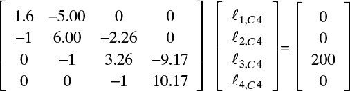
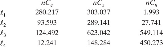
Calculate matrix variables A, B, C, and D for each component (see Table 6-2 for n-C4 solution).
Intermediate values for the Thomas algorithm are:
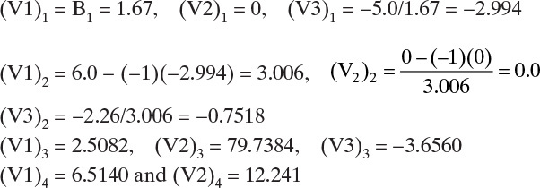
Then flow rates n-C4 are
Calculate mole fractions on each stage.
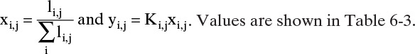
TABLE 6-2. Matrix calculations for Example 6-1 for n-C4
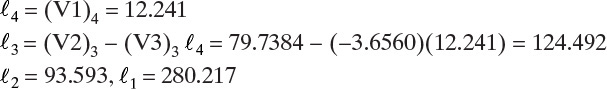
Invert the tridiagonal matrix with either a spreadsheet or the Thomas algorithm (shown here). The Thomas parameters for each component (see Table 6-2 for n-C4 solution) are
Calculate the component flow rate on each stage for each component (see Table 6-2 for n-C4 solution):
![]() 4 = (V2)4,
4 = (V2)4, ![]() 3 = (V2)3 – (V3)3
3 = (V2)3 – (V3)3![]() 4
4
![]() 2 = (V2)2 – (V3)
2 = (V2)2 – (V3) ![]() 3,
3, ![]() 1 = (V2)1 – (V3)1
1 = (V2)1 – (V3)1![]() 2
2
The results are
Calculate normalized values for component mole fractions on each stage:
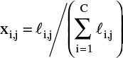
See Tables 6-2 and 6-3.
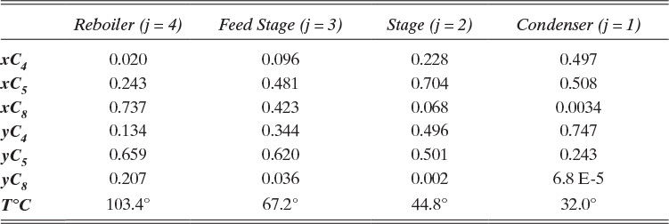
Calculate the temperature on each stage with a bubble-point calculation.
Reboiler (j = 4). Converges to T = 103.4°C. Then the vapor mole fractions are
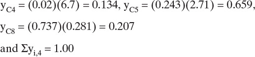
Other calculations are summarized in Table 6-3.
At this point we would use these temperatures to determine new K values and then repeat the matrix and bubble-point calculations. To speed convergence, process simulators use more advanced methods for determining the next set of temperatures (see Section 6.6). Obviously, with this amount of effort we would prefer to use a process simulator to solve the problem (see Problem 6.G1). The process simulator results for temperature are generally higher than the temperatures calculated in this example after one iteration, except for stage 1, which has a calculated temperature that is too high. In addition, since this system does not follow CMO, there is considerable variation in the flow rates.
6.5 Energy Balances in Matrix Form
After convergence of the temperature loop, the liquid and vapor flow rates, Lj and Vj, can be corrected using energy balances (see Figure 6-1). For the general stage shown in Figure 6-3, the energy balance is
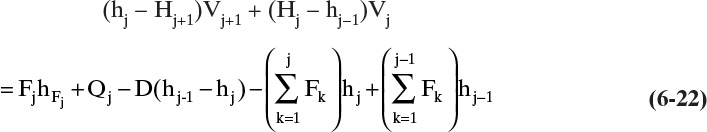
This equation is for 2 ≤ j ≤ N – 1. The liquid flow rates can be substituted in from a mass balance around the top of the column:
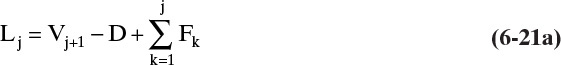
where 2 ≤ j ≤ N – 1.
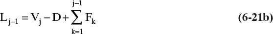
Substituting Eqs. (6-21a) and (6-21b) into Eq. (6-20) and rearranging, we obtain
For a total condenser since V2 = L1 + D and h1 = hD, the energy balance is
For the partial reboiler (j = N), the energy balance is
and the overall flow rate can be calculated from
Substituting Eq. (6-26) into (6-25) and rearranging, we have
If Eqs. (6-22), (6-24), and (6-27) are put in matrix form, we have
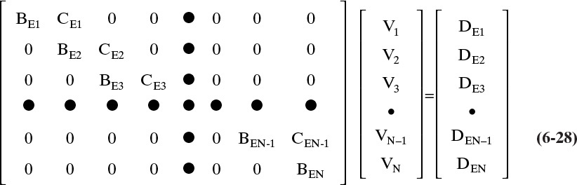
This EB matrix again has a tridiagonal form (with Aj = 0) and can be inverted to obtain the vapor flow rates. The BE and CE coefficients in Eq. (6-28) are obtained by comparing Eqs. (6-22), (6-24), and (6-27) to Eq. (6-28). For j = 1 these values are
For 2 ≤ j ≤ N – 1
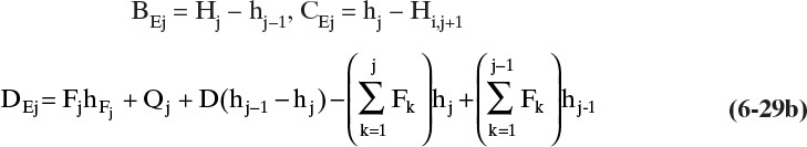
and for j = N
The coefficients in Eqs. (6-29) require knowledge of the enthalpies leaving each stage and the Q values. The enthalpy values can be calculated since all x’s, y’s, and temperatures are known from the component mass balances and the converged temperature loop. For ideal mixtures, the enthalpies are
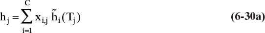
and
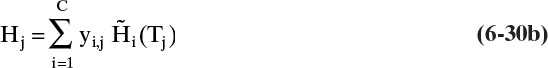
where ![]() and
and ![]() are the pure component enthalpies.
are the pure component enthalpies.
They can be determined from data (e.g., see Maxwell, 1950, or Smith, 1963) or from heat capacities and latent heats of vaporization.
Usually the column is adiabatic. Thus,
The condenser requirement can be determined from balances around the total condenser:

Since D and L/D are specified and hD and H2 can be calculated from Eqs. (6-30), Q1 can be determined. For an adiabatic column, the reboiler heat load can be calculated from an overall energy balance.

Inversion of Eq. (6-28) gives new guesses for all the vapor flow rates. The liquid flow rates can then be determined from mass balances, such as Eqs. (6-21) and (6-26). These new liquid and vapor flow rates are compared to the values used for the previous convergence of the mass balances and temperature loop. The check on convergence is if
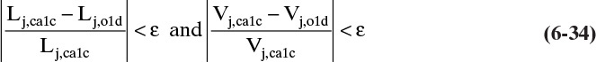
for all stages, then the calculation has converged. For computer calculations, an ε of 10–4 or 10–5 is appropriate.
If the problem has not converged, the new values for Lj and Vj must be used in the mass balance and temperature loop (see Figure 6-1). Direct substitution is the easiest approach. That is, use the Lj and Vj values just calculated for the next trial.
When Eqs. (6-34) are satisfied, the calculation is finished because the mass balances, equilibrium relationships, and energy balance have all been satisfied. The solution gives the liquid and vapor mole fractions, flow rates, and the temperature on each stage and in the products.
6.6 Introduction to Naphtali-Sandholm Simultaneous Convergence Method
One of the more robust methods for solution of multicomponent distillation and absorption problems is developed in a classic paper by Naphtali and Sandholm (1971). This method is available in many commercial simulators. Naphtali and Sandholm developed a linearized Newtonian method to solve all the equations for multicomponent distillation simultaneously.
The Newtonian procedure outlined in Eqs. (2-50) to (2-55) for the energy balance for flash distillation can be considered a simplified version of the method used by Naphtali and Sandholm. I recommend that students reread that material before proceeding.
To develop a simultaneous Newtonian procedure for multicomponent distillation, Naphtali and Sandholm (1971) first wrote the N(2C + 1) equations and variables consisting of component mass balances [essentially Eq. (6-13) but without substitution of the equilibrium K values for yi], the energy balances [essentially Eq. (6-28)], and the equilibrium relationships, including Murphree vapor efficiencies in functional matrix form. Their procedure is illustrated for the energy balance. Essentially, the functional matrix form for Eq. (6-28) is

When you first start the calculation with the initial guesses for all temperatures and vapor and liquid flow rates, the energy balance, component mass balance, and equilibrium functions will not equal zero. The Newtonian method is used to develop new values for the variables to calculate enthalpies and K values. To use the Newtonian method, Naphtali and Sandholm developed derivatives for the changes in all variables. Note that the energy balance (and component mass balances and equilibrium relationships) on plate j depend only on the variables on plates j–1, j, and j+1. For the energy balance function on plate j, the derivatives with respect to the variables on plate j–1 are
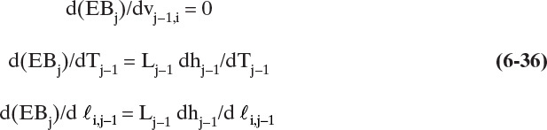
where vj–1,i = Vj–1 yj–1,i. The derivatives for energy balance on plate j with respect to the variables on plate j are

And the derivatives for the energy balance function on plate j with respect to the variables on plate j+1 are
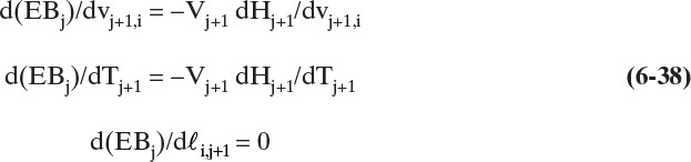
These equations extend Eq. (2-52), developed for multicomponent flash distillation, to multicomponent column distillation.
The next value for every variable is the old value plus the calculated correction. For example, for temperature on stage j, the value for the next trial is
where the correction ΔTj is determined from the Newtonian approximation
where [Fold] is the combined matrix of all functions (energy balance, component mass balances, and equilibrium) and [(dF/dT)old] is the combined matrix of all the derivatives, since temperature affects all of these functions. Equation (6-40) is an extension of Eq. (2-51) to a multistage distillation with multiple variables. This procedure is followed for every variable (Tj, vi,j, and ![]() i,j on every stage j) to obtain new values for each variable. These new values are used in the next trial to calculate the values of the energy balance, component mass balance, and equilibrium functions. These functions should all have a value of zero, and their differences from zero are the discrepancies in the answer. The convergence check is that the sum of squares of the discrepancies is less than some tolerance, such as 10–7.
i,j on every stage j) to obtain new values for each variable. These new values are used in the next trial to calculate the values of the energy balance, component mass balance, and equilibrium functions. These functions should all have a value of zero, and their differences from zero are the discrepancies in the answer. The convergence check is that the sum of squares of the discrepancies is less than some tolerance, such as 10–7.
6.7 Discussion
All of the methods for solving multicomponent distillation and absorption problems have weaknesses. The bubble-point method works well for narrow-boiling feeds, but is inherently unstable for wide-boiling feeds. The sum-rates method (Section 12.9) works well for wide-boiling feeds such as most absorbers but is unstable for narrow-boiling feeds. The Naphtali-Sandholm approach often works well for both narrow- and wide-boiling feeds, but Newtonian methods are notorious for diverging for nonlinear problems if the first guess is not close to the final answer. Since distillation problems can be extremely nonlinear, the first guess can be very important for all of these methods. If a good first guess is difficult to find, try finding a simpler set of conditions in which convergence does occur (e.g., fewer stages or larger L/D) and then approach the desired condition by slowly changing the values of the variables. Since commercial simulators use the previous run as an initial guess for the current run, this method should make the initial guess closer to the answer, which means convergence is more likely.
A number of methods to make the convergence schemes more stable have been developed and are employed in commercial process simulators. As a result, commercial simulators are quite robust, particularly if an appropriate method (bubble-point, sum-rates, or Naphtali-Sandholm) is chosen and a good first guess has been used, although they occasionally still have difficulty converging. When there is a convergence difficulty, first check that the basic solution approach chosen appears to be appropriate. Then try increasing the number of iterations allowed. If this does not work, try reducing the tolerance on convergence. Finally, most simulators have a number of options to make convergence more stable, such as damping the predicted change in variables, and these options can be tried. With a combination of these approaches, almost all equilibrium-staged multicomponent distillation problems can be solved. This is one of the great advances in chemical engineering in the past 100 years. Rate-based models for distillation are considered in Chapter 16.
The matrix approach is easily adapted to partial condensers and to columns with sidestreams (see Problems 6.C2 and 6.C1). The approach converges for normal distillation problems. Extension to more complex problems, such as azeotropic and extractive distillation or very wide boiling feeds, is beyond the scope of this book; however, these problems are solved with a process simulator in Chapter 8.
In some ways, the most difficult part of writing a multicomponent distillation program has not been discussed in detail. This is the development of a physical properties package that will accurately predict equilibrium and enthalpy relationships (Barnicki, 2002; Carlson, 1996; Poling et al., 2001; Sadeq et al., 1997; Schad, 1998). Sadeq et al. (1997) compared three process simulators and found that relatively small differences in the parameters and in the VLE correlation can cause major errors in the results. Fortunately, a considerable amount of research has been done (see Table 2-2; Fredenslund et al., 1977; and Walas, 1985) to develop accurate physical property correlations. Very detailed physical properties packages can be purchased commercially and are included in the commercial process simulators.
Most companies using distillation have computer programs available using one of the advanced calculation procedures. Several software and design companies sell these programs. Typical engineers use these routines and do not go through the effort required to write their own routines. However, an understanding of the expected profiles and the basic mass and energy balances in the column can be very useful in interpreting the computer output and in determining when that output is garbage. Thus, it is important to understand the principles of distillation calculations even though the details of the computer program may not be understood.
References
Amundson, N. R., and A. J. Pontinen, “Multicomponent Distillation Calculations on a Large Digital Computer,” Ind. Engr. Chem, 50, 730 (1958).
Barnicki, S. D., “How Good Are Your Data?” Chem. Engr. Progress, 98 (6), 58 (June 2002).
Carlson, E. C., “Don’t Gamble with Physical Properties for Simulations,” Chem. Engr. Progress, 92 (10), 35 (Oct. 1996).
Fredenslund, A., J. Gmehling, and P. Rasmussen, Vapor-Liquid Equilibria Using UNIFAC: A Group-Contribution Method, Elsevier, Amsterdam, 1977.
Holland, D. D., Fundamentals of Multicomponent Distillation, McGraw-Hill, New York, 1981.
King, C. J., Separation Processes, 2nd ed., McGraw-Hill, New York, 1981.
Lapidus, L., Digital Computation for Chemical Engineers, McGraw-Hill, New York, 1962.
Maxwell, J. B., Data Book on Hydrocarbons, Van Nostrand, Princeton, NJ, 1950.
Naphtali, L. M., and D. P. Sandholm, “Multicomponent Separation Calculations by Linearization,” AIChE Journal, 17 (1), 148 (1971).
Poling, B. E., J. M. Prausnitz, and J. P. O’Connell, The Properties of Gases and Liquids, 5th ed., McGraw-Hill, New York, 2001.
Sadeq, J., H. A. Duarte, and R. W. Serth, “Anomalous Results from Process Simulators,” Chem. Engr. Education, 31 (1), 46 (Winter 1997).
Schad, R. C., “Make the Most of Process Simulation,” Chem. Engr. Progress, 94 (1), 21 (Jan. 1998).
Seader, J. D., E. J. Henley, and D. J. Roper, Separation Process Principles, 3rd ed., Wiley, New York (2011).
Smith, B. D., Design of Equilibrium Stage Processes, McGraw-Hill, New York, 1963.
Walas, S. M., Phase Equilibria in Chemical Engineering, Butterworth, Boston, 1985.
Wankat, P. C., Equilibrium-Staged Separations, Prentice Hall, Upper Saddle River, NJ, 1988.
Homework
A. Discussion Problems
A1. In the matrix approach, we assumed K = K (T, p). How would the flowchart in Figure 6-1 change if K = K (T, p, xi)?
A2. The method described in this chapter is a simulation method because the number of stages and the feed and withdrawal locations must all be specified. How do you determine the optimum feed stage?
A3. Develop your key relations chart for this chapter.
A4. In a multicomponent simulation program for distillation, the loops are nested. The outermost loop is mole fractions, next is flow rates, and the innermost loop is temperature.
1. Mole fractions are the outermost loop because:
a. Many distillation problems can be done without this loop.
b. Changing mole fractions often do not have a major effect on K values.
c. Mole fractions have a major impact on K values only for systems with complex equilibrium behavior.
d. All of the above.
2. The temperature loop is done before the flow rate loop because:
a. Temperatures cannot be constant in distillation.
b. Flow rates are often very close to constant in each section of the column.
c. A very good guess of flow rates can be made.
d. All of the above.
3. A good initial guess of the flow rates is to:
a. Assume CMO.
b. Assume the liquid and vapor flow rates are constant throughout the column.
c. Use a bubble-point calculation at the top and bottom of the column.
4. For a good initial guess of temperatures:
a. Assume CMO.
b. Use any arbitrary temperature.
c. Use a bubble-point calculation at the top and bottom of the column.
5. The mass balances are solved by developing a matrix that is then inverted. The matrix allows one to have feed at:
a. Only one location in the column.
b. Two locations in the column.
c. Any stage within the column but not at the condenser and the reboiler.
d. Any stage in the column and at the reboiler and the condenser.
A5. The method described in this chapter is a simulation method because the number of stages and the feed and withdrawal locations must all be specified. How do you determine if you have enough stages for a design problem?
A6. Since a new liquid flow rate is calculated in Eq. (6-17) as  , why do we not set Lj,new equal to this value instead of reverting back to Lj,old after calculating the liquid mole fractions?
A7. The enthalpies in Eqs. (6-30a) and (6-30b) assume ideal mixtures. How do the equations change if the mixtures are not ideal? Do you expect that the deviation from ideal mixture behavior will be larger for liquid enthalpy or for vapor enthalpy?
C. Derivations
C1. Suppose there is a liquid sidestream of composition xi,s = xi,j and flow rate Sj is removed from stage j in Figure 6-3.
a. Derive the mass balance Eqs. (6-4) to (6-6) for this modified column.
b. Develop new energy balance equations. Derive new coefficients for Eq. (6-29b).
C2. Derive the mass balance expression for the matrix approach if there is a partial condenser instead of a total condenser. Replace Eqs. (6-7) to (6-9).
C3. Derive the energy balance expression for the matrix approach if there is a partial condenser instead of a total condenser. Replace Eqs. (6-23), (6-24), and (6-29a).
C4. Suppose there is a total reboiler instead of a partial reboiler. Eqs. (6-10) to (6-12) will be changed and the neat logic of the tridiagonal matrix does not work as well.
a. Derive the mass balance matrix if FN = 0.
b. Determine how to arrange the calculations to do the mass balances when FN ≠ 0, zN ≠ xN–1, and the feed to the total reboiler is a liquid that we desire to vaporize.
D. Problems
*Answers to problems with an asterisk are at the back of the book.
D1. For the first trial of Example 6-1 determine the component matrix for n-pentane and then use the Thomas algorithm to find the n-pentane liquid flow rates leaving each stage. Compare your n-pentane flow rates with the values given in Example 6-1.
D2. We are separating a mixture of ethane, propane, n-butane, and n-pentane in a distillation column operating at 5.0 atm. The column has a total condenser and a partial reboiler. The feed flow rate is 1000.0 kmol/h. The feed is a saturated liquid. Feed is 8.0 mol% ethane, 33.0 mol% propane, 49.0 mol% n-butane, and 10.0 mol% n-pentane. The column has 4 equilibrium stages and the partial reboiler, which is an equilibrium contact. The feed is on second stage below the total condenser. The reflux ratio L0/D = 2.5. Distillate flow rate D = 410 kmol/h. Develop the mass balance and equilibrium matrix (Eq. 6-13) with numerical values for each element (Aj, Bj, Cj, and Dj). Do this for your first guess: Tj = bubble-point temperature of feed (use the same temperature for all stages); K values are from the DePriester chart; and L and V are CMO values. Do the matrix for propane only.
D3. Do the matrix for n-butane for Problem 6.D2.
D4. A distillation column is separating 100.0 kmol/h of a saturated liquid feed that is 30.0 mol% methanol, 25.0 mol% ethanol, 35.0 mol% n-propanol, and 10.0 mol% n-butanol at a pressure of 1.0 atm. The column has a total condenser and a partial reboiler. We want a 98.6% recovery of n-propanol in the distillate and 99.2% recovery of n-butanol in the bottoms (but realize that this first trial will not provide this amount of separation). Operation is with L/D = 5, D = 60, N = 4, and Nfeed = 3 (#1 = total condenser, and #4 = partial reboiler). Set up the mass balance matrix Eq. (6-13) for the first trial for n-butanol and then solve. This is a hand calculation.
a. Use CMO to estimate liquid and vapor flow rates in the column for the first trial. Report these flow rates.
b. For a first guess of K values, assume the K values in the column are constant and equal to those found in a bubble-point calculation for the feed. The Knp values are (y/x)np where ynp and xnp are from the bubble-point calculation with constant alpha, Eq. (5-28) in Problem 5.C1. The other Ki = αi Knp.
c. Calculate all the A, B, C, and D values (but for n-butanol only), and write the complete matrix.
d. Solve the n-butanol matrix using the Thomas algorithm, and find the n-butanol flow rates, ![]() n-C4,j, leaving each stage.
n-C4,j, leaving each stage.
e. The T implicitly used in the calculation to find the K values is the bubble-point temperature of the feed. To determine T, first calculate the K value for n-propanol as (y/x)n–propanol where y and x are found from the constant relative volatility solution for the bubble point. Then use Raoult’s law to find the T that gives this K value. Report this temperature.
Do not do additional trials.
System properties: If we choose n-propanol as the reference, the relative volatilities are methanol = 3.58, ethanol = 2.17, n-propanol = 1.0, and n-butanol = 0.412. These relative volatilities can be assumed to be constant. The K value for n-propanol can be estimated from Raoult’s law. The vapor pressure data (in mm Hg) for n-propanol from Perry’s Chemical Engineers’ Handbook is:

D5. Repeat Problem 6.D4 except do the matrix and solution for the first trial for methanol.
F. Problems Requiring Other Resources
F1.* A distillation column with two stages, a partial reboiler, and a partial condenser is separating benzene, toluene, and xylene. The feed rate is 100.0 kmol/h, and the feed is a saturated vapor introduced on the bottom stage of the column. Feed compositions (mole fractions) are zB = 0.35, zT = 0.40, zX = 0.25. The reflux is a saturated liquid, and p = 16.0 psia. A distillate flow rate of D = 30.0 kmol/h is desired. Assume Ki = VPi/p. Do not assume constant relative volatility, but do assume CMO. Use the matrix approach to solve mass balances and the bubble-point method for temperature convergence. For the first guess for temperature, assume that all stages are at the dew-point temperature of the feed. Do only one iteration. See Problem 6.C2 for handling the partial condenser.
G. Computer Simulation Problems
G1. Use a process simulator to completely solve Example 6-1. Do not assume CMO. Compare temperature and mole fractions on each stage to the values obtained in Example 6-1 after one trial.
G2. You have an ordinary, single-feed distillation column separating ethane, propane, n-pentane, and n-hexane. In Aspen notation N = 21; the feed location in the column is Nfeed = 10 (input above stage); the reflux ratio is 2.0; pressure is 5.0 atm (operate the column at constant pressure); there is a partial vapor condenser with saturated liquid reflux and a kettle-type reboiler; the feed flow rate is 100.0 kmol/h; feed mole fractions are ethane = 0.25, propane = 0.36, n-pentane = 0.29, n-hexane = 0.10; feed pressure is 5.0 atm; and the fraction of feed vaporized is 0.3. D = 25.0 kmol/h and is entirely a vapor, column is adiabatic, and you should use the Peng-Robinson VLE package. Open a new blank file, simulate this system, and answer the following questions:
1. Record the following values:
a. Temperature of condenser (°C)
b. Temperature of reboiler (°C)
c. Temperature of feed (°C)
d. Qcondenser (cal/s)
e. Qreboiler (cal/s)
f. Distillate product mole fractions
g. Bottoms product mole fractions
2. Was the specified feed stage the optimum feed stage? Yes No
If no, the feed stage should be: (a) closer to the condenser, or (b) closer to the reboiler.
(Note: Do the minimum number of simulations to answer these questions. Do not optimize.)
3. Which tray gives the largest column diameter with sieve trays when you use the originally specified feed stage? Aspen notation #__________. Column diameter = __________ m.
[Use the default values for number of passes (1), tray spacing (0.6096 m), minimum downcomer area (0.10), foaming factor (1), and over-design factor (1). Set the fractional approach to flooding at 0.7. Use the “Fair” design method for flooding.]
4. Which components in the original problem are the key components (label LKs and HKs)?
5. Change either D or B to make propane LK and n-butane HK. Pick a value that gives a very high yield of propane in the distillate and a very high yield of n-pentane in the bottoms. Note: Distillate remains entirely a vapor. Use the same N and feed stage as original.
a. What operating parameter did you change, and what is its new value?
Record the following values:
b. Temperature of condenser (°C)
c. Temperature of reboiler (°C)
d. Distillate product mole fractions
e. Bottoms product mole fractions
G3. Use a process simulator to simulate the separation of a mixture that is 0.25 mole fractionmethanol, 0.30 mole fraction ethanol and 0.45 mole fraction n-propanol in a series oftwo distillation columns. The feed rate is 100 kmol/h and the feed is at 50°C and 1.0 atm.The feed goes to the first column, which has 22 equilibrium stages, a total condenser, anda kettle reboiler; on (above) stage 11 below the condenser. The distillate from this column, containing mainly methanol and ethanol is fed to the second column. Set the D value to 55.0. Vary L/D in the first column to achieve a 0.990 or better split fraction of ethanol in the distillate and a 0.990 or better split fraction of n-propanol in the bottoms.Vary L/D by increments of 0.1 (e.g., L/D = 0.8, 0.9, 1.0, and so forth) until you find the lowest L/D that gives the desired separation. (You can start with any L/D value you wish.) Both columns are at 1.0 atm pressure. Use the Wilson VLE package.
For column 1 report the following:
a. Final value of L/D ___________________________
b. Split fractions of ethanol (distillate)_________and n-propanol (bottoms) __________
c. Mole fractions in bottoms _____________________________________________
d. Mole fractions in distillate _____________________________________________
The second column receives the distillate from column 1 as a saturated liquid feed at oneatm. pressure. The second column is at 1.0 atm pressure and operates with D = 25.0 and L/D = 4.0. It has a total condenser and a kettle reboiler. There are 34 equilibrium stages in the column. Find the optimum feed stage location. For column 2 report the following:
a. Optimum feed location in the column___________________________
b. Mole fractions in bottoms ____________________________________________
c. Mole fractions in distillate ___________________________________________
G4. The feed mole fractions are methanol = 0.2, ethanol = 0.5, and 1-propanol = 0.3. The feed is at 75°C, the flow rate is 1000.0 kmol/h, and pressure is at 1.0 bar. We want each product to have mole fraction of 0.99 or greater. Use Figure 11-6A (methanol product distillate from the first column, ethanol product distillate from second column, and 1-propanol product bottoms from second column). Operate both columns at a constant pressure of 1.0 bar. Both columns have total condensers and kettle-type reboilers. Each column has only one feed. Column 1 has N (Aspen notation) = 40. Column 2 has reflux ratio = 2.0.
Preliminary. What VLE correlation will you use and why?
First, find conditions that give methanol, ethanol, and 1-propanol products that are all 99.0 mol% or greater. Record the conditions that worked:
Column 1. Aspen N = 40 (given), Aspen feed location = ______, operating condition 1 on the Setup-Configuration tab __________ (e.g., distillate flow rate) and value __________; operating condition 2 on the Setup-Configuration tab __________ and value __________
Column 2. Aspen N = _____, Aspen feed location = ______, operating condition 1 on the Setup-Configuration tab __________ (e.g., distillate flow rate) and value __________reflux ratio = 2.0 (specified).
Initial results:
Methanol mole fraction in methanol product: __________
Ethanol mole fraction in ethanol product: __________
1-propanol mole fraction in 1-propanol product: __________
Second, for column 1, keep all variables except for the reflux ratio and the feed location constant. Find the optimum feed location for N = 40. Then with N =40 and the optimum feed stage, find the lowest reflux ratio that gives the methanol mole fraction within the range 0.99000 to 0.99004.
Column 1. Aspen N = 40 (specified), Aspen optimum feed location = ______, reflux ratio = __________, Methanol mole fraction in methanol product __________.
Third, with changes in column 1, the products from column 2 may no longer meet specifications. If this is the case, find conditions that work but keep the reflux ratio = 2.0 and do not change column 1. If column 2 already meets the specifications or once column 2 meets the specifications, keep all variables except for N and the feed location constant. Find the optimum feed location. Reduce N as much as possible while using the optimum feed location and obtaining ethanol and 1-propanol product mole fractions that are greater than or equal to 0.99000.
Column 2. Aspen N = _____, Aspen optimum feed location = ______, operating condition 1 on the Setup-Configuration tab __________ (e.g., distillate flow rate) and value __________; reflux ratio = 2.0.
Ethanol mole fraction in ethanol product: __________
1-propanol mole fraction in 1-propanol product: __________
G5. You have an ordinary, single-feed distillation column separating benzene, toluene, cumene, p-xylene (the last one is paraxylene, C8H10). There are 23 trays in the column; the feed location in column is tray 12 (input above stage); the reflux ratio is 4.0; pressure is at 3.0 atm (operate column at constant pressure); there is a total condenser with a saturated liquid reflux and a kettle-type reboiler; feed flow rate is 400.0 kmol/h; feed mole fractions are benzene = 0.2, toluene = 0.45, p-xylene = 0.35; feed pressure is 3.0 atm; feed temperature is 100°C; D = 80 kmol/h; column is adiabatic; and you should use the Peng-Robinson VLE package. Open a new blank file, simulate this system with RadFrac, and answer the following questions:
1. Report the following values:
a. Temperature of condenser (K)
b. Temperature of reboiler (K)
c. Qcondenser (cal/sec)
d. Qreboiler (cal/sec)
e. Distillate product mole fractions
f. Bottoms product mole fractions
2. Was the specified feed stage the optimum feed stage? Yes No
If no, the feed stage should be: (a) closer to the condenser, (b) closer to the reboiler.
(Note: Do minimum number of simulations to answer these questions. Do not optimize.)
3. Which tray gives the largest column diameter with sieve trays when one uses the originally specified feed stage? Aspen Tray #__________, Column diameter = __________ m
Use the default values for number of passes (1), tray spacing (0.6096 m), minimum downcomer area (0.10), foaming factor (1), and over-design factor (1). Set the fractional approach to flooding at 0.7. Use the Fair design method for flooding.
4. Which components in the original problem are the key components (label LKs and HKs)?
5. Change one specification in the operating conditions (keep N, original feed location, feed flow rate, feed composition, feed pressure, feed temperature or fraction vaporized constant) to make toluene the LK and p-xylene the HK.
a. What operating parameter did you change, and what is its new value?
Record the following values:
b. Temperature of condenser (K)
c. Temperature of reboiler (K)
d. Distillate product mole fractions
e. Bottoms product mole fractions
Chapter 6 Appendix. Computer Simulations for Multicomponent Column Distillation
Lab 4. Simulation of Multicomponent Distillation
Goal:
Explore simulation of multicomponent distillation with Aspen Plus.
Preparation:
• Review procedures for starting Aspen Plus (Computer Labs 1 and 2)
• Review specific directions for distillation covered in Computer Lab 3
Aspen Plus uses the same calculation methods for binary and multicomponent distillation, but some differences will become apparent as you proceed through this lab.
1. Input a saturated vapor feed at 1.0 bar that consists of n-butane, 20.0 kmol/h; n-pentane, 30.0 kmol/h; and n-hexane, 50.0 kmol/h.
2. Pick an appropriate VLE package to use, and check the equilibrium predictions [e.g., K values should be reasonably close to the predictions made with the DePriester charts (Figures 2-10 and 2-11), but note that the empirical correlation (Eq. 2-28) is not more accurate than the DePriester charts].
3. Place a RadFrac distillation column on the main flowsheet. Connect a feed stream, a bottoms product stream, and a vapor distillate product instead of a liquid distillate product. When done, click Next.
4. In the Block for the column in the Configuration tab, choose the following from the Setup Options menu:
a. Calculation Type: Equilibrium
b. Number of Stages: 40 (this is only an initial setting)
c. Condenser: Partial-Vapor
d. Reboiler: Kettle
e. Valid Phases: Vapor-Liquid
f. Convergence: Standard
5. If you get an error in step 4, chances are you have a liquid distillate in the drawing and are trying to take a vapor distillate product (i.e., Condenser: Partial-Vapor). Redraw your column with a vapor distillate stream. (You can confirm connections by selecting the stream and then hovering the mouse over the blue connection area. A balloon will appear with the connection details.)
6. Complete the Configuration window by selecting Operating Specifications.
a. Select Reflux ratio from the menu, and use a value of 3.0 (more than sufficient for this separation).
b. Adjust the value of Distillate rate (or Bottoms rate) to make the butane and pentane exit from the top of the column and the hexane from the bottom. This can be done by setting D (or equivalently B) so that an external mass balance will be satisfied if a perfect split is achieved (e.g., butane recovery in distillate of 100%, pentane recovery in distillate of 100%, and hexane recovery in the bottoms of 100%)
7. The Streams tab and the Pressure tab need values or RadFrac will not run.
a. In the Streams tab select feed on stage 20, Convention = vapor (select from menu).
b. In the Pressure tab initially try a pressure of 1.0 bar in stage 1. Leave the other pressures blank–RadFrac will use a constant column pressure of 1.0 bar.
8. Click Next and then click OK if the message states the required input is complete and asks if you want to run the separation. The calculations are typically very fast.
9. In the menu at the top of the Navigation Pane on the left side of the screen, click Results Only. Then in the list of items for your distillation block click Results.
a. From the Summary tab record the temperatures of the distillate and bottoms.
b. Record the heat loads in the condenser and the reboiler in kW. (Place the cursor on the units for heat duty, and use the menu to select kW.)
c. Click the Split Fraction tab, and record the values (also called fractional recoveries).
10. In the Navigation Pane (menu lists Results Only), in the list of items for your distillation block, click Profiles.
a. In the TPFQ tab note the temperatures of the stages. The presence of a number of stages with almost the same temperature is an indication that there are pinch points in the column. In this case the constant temperature regions occur because more stages are used than needed.
b. In the TPFQ tab of Profiles look at the vapor and liquid flow rates. Is CMO valid? Determine how much L/V varies in the rectifying and in the stripping sections. Look immediately above and below the feed stage.
c. In the Composition tab record the mole fractions of the components in the distillate and bottoms. Use the menu to change from vapor to liquid. Note that for this simulation distillate is a vapor, and bottoms is a liquid. Be sure that the second menu is set for moles (default is mass).
11. Change the settings so that the butane exits the top and the pentane and hexane the bottoms (change D or B to do this). Under these conditions you should get an error message that the column dried up. Why did this happen? Change the feed to a saturated liquid feed (V/F = 0 in feed), and run it again with the changed setting for D or B.
12. Try an intermediate cut where butane exits from the top, hexane from the bottom, and pentane distributes between the top and bottoms (change D or B). Use a saturated liquid feed. Compare QC and QR in this and the previous run (6 and 7). Explain.
13. Continue with the result from step 11 (V/F = 0 in the feed). Find the total number of stages and the optimum feed location if we want the n-butane mole fraction in the bottoms to be 0.00100 or less and the n-pentane mole fraction in the distillate to be 0.00100 or less. This calculation is trial-and-error in Aspen Plus. Since Aspen Plus calls the partial condenser 1, the vapor composition leaving stage 1 is the distillate, and the last liquid mole fraction is the bottoms. Is it more difficult to meet the C4 or the C5 requirement?
14. Record your condenser and reboiler temperatures for step 13 from the TPFQ tab of Profiles. The condenser temperature is low enough that refrigeration is needed. This is expensive. To avoid this, raise the column and feed pressures until the condenser temperature is high enough that cooling water can be used for condensation. (Use a cooling water temperature of 30°C, and add 5°C for the approach temperature in the heat exchanger.) Changing the pressure changes the VLE. Check to see if you still have the desired separation (the same as in step 13). If not, find the new values for the optimum feed and the total number of stages to obtain the desired mole fractions. Be sure to raise your feed pressure so that it is equal to the column pressure. Why are more stages required at the higher pressure?
15. Try different values for L/D or boilup ratio. See how this affects the separation. Try using different operating specifications in RadFrac.
16. Now try a feed temperature of 30°C (but the same concentrations and pressure) at conditions that you optimized previously. Look at how the reboiler and condenser heat loads change, and compare them to the results from step 9. Try changing the feed composition (remember to change D or B to satisfy mass balances.)
17. Try a different feed flow rate (but the same concentrations and fraction vapor) at conditions that you optimized previously. The number of stages, optimum feed location, and separation achieved should not change. The heat requirements will be different, as will outlet flow rates. Compare QR/(feed rate) for the two runs. What does this say about the design of distillation for different flow rates?
18. Change the column configuration, and have a liquid distillate product. This requires redrawing your flowsheet. Compare the results to the results of step 14, but remember the distillate is now a liquid.
19. Click Properties (lower left of Aspen Plus screen) and then in the Home toolbar click Residue Curves (far right side of toolbar in the Home tab). If you get a Popup message titled “Distillation Synthesis” click Continue to Aspen Plus Residue Curves. Set the pressure you want, and click Run Analysis. This gives a residue curve for your chemical system. A residue curve (Section 8.5.2) shows the path that a batch distillation will follow for any starting condition. The absence of nodes and azeotropes for this nearly ideal chemical system shows that the designer can obtain either the lightest or the heaviest species as pure products for any feed concentration. This is not true when there are azeotropes.
20. Switch chemical systems, and try the more complicated chemical system methanol-ethanol-water at 1 atm. (In the Properties menu go to Components→Specifications. Left-click the arrow by each component and then right-click to get a menu. Delete the rows and then add the three components. Aspen will ask if you want the parameters updated. Click yes; however, Aspen assumes you still want to use Peng-Robinson, which is not the best choice. In the Properties menu [All Items] go to Methods→Specifications. In the Global Tab in the menu for Method Name select NRTL-2. Click Next until you are past the interaction parameters.) Then look at the residue curve map. Expand the size of the map, and look for the ethanol-water azeotrope (where one of the curves intersects the side of the triangle running from ethanol to water.) Try simulating a distillation column with this system.
21. Feel free to further explore Aspen Plus on your own.
Lab 5. Pressure Effects and Tray Efficiencies
In this lab we continue to use RadFrac to explore distillation in more detail and to learn more about the capabilities of Aspen Plus.
Goal:
Explore the simulation of multicomponent distillation with Aspen Plus as a continuation of Labs 3 and 4 using RadFrac to explore distillation in more detail and to learn more about the capabilities of Aspen Plus.
Preparation:
• If necessary review the procedures for starting Aspen Plus (Labs 1 and 2)
• Review the specific directions for distillation covered in Labs 3 and 4
For parts I, II, III, and IV use the following feed:
• 100.0 kmol/h at 20°C
• Mole fractions of components are: ethane 0.091, ethylene 0.034, propane 0.322, propylene 0.064, n-butane 0.413, n-pentane 0.057, and n-hexane 0.019.
• Use Peng-Robinson for VLE.
• Pressure of the feed should be 0.1 atm above that of the column.
• The column has a total condenser and a partial reboiler.
• There is a single feed, a liquid distillate, and a liquid bottoms.
Draw the flowsheet, and input all data. Then save the file. For part I record the mole fractions of n-butane in distillate and propane in bottoms. Record the temperatures and the K values for n-butane and propane in the reboiler and the condenser.
I. Pressure Effects—Temperatures
a. Suppose we want to split between the C3 and the C4 components. Set D = 51.1 kmol/h (Why is this value selected?), p = 1.0 atm, N = 30.0 (includes reboiler and condenser), Nfeed = 15.0, L/D = 2.0. Record distillate and bottoms purities and condenser and reboiler temperatures. If convergence is a problem, in the Column Block Configuration tab, change Convergence from Standard to Petroleum/Wide-boiling.
b. Repeat run step Ia but at p = 10.0 atm. Record the same items as in part Ia.
c. Since cooling water is much cheaper than refrigeration, we want to operate with the condenser at a temperature that is high enough that cooling water can be used. Assume the minimum temperature is 35°C (30°C cooling water plus 5°C approach in heat exchanger). Have we satisfied this for either run? If not, what is the lowest pressure that produces a cooling water temperature of 30°C? Try 20.0 atm and go down. For your final pressure record the same data as in part Ia.
d. Compare the mole fractions of distillate and bottoms for parts a, b, and c.
Reduction in pressure is used if the reboiler temperature would be too high or if there is excessive thermal degradation.
II. Pressure Effects—Changing Split
Suppose we want to split between the C2 and C3 components (ethane and ethylene are in the distillate, and everything else in bottoms). Change the value for the distillate flow rate in Aspen Plus to achieve this. Operate at pressure of 20.0 atm. Except for distillate flow rate, use the same settings as previously used. Run Aspen Plus, and compare the temperature in the condenser to the temperature in run step Ic (also at 20.0 atm). What can you conclude? Record distillate and bottoms mole fractions and temperatures.
III. Pressure Effects—Column Diameter
Note: Do part IV at the same time as part III.
Aspen Plus will size the column diameter and set up the tray dimensions. In the Navigation Pane (All Items list) find the block for your distillation column, and click Sizing and Rating. Then click on the file Tray Sizing. Click New (or Edit if you have previously set this up) and then OK for section 1. Section 1 can be the entire system—stages 2 to 29 (remember that Aspen Plus calls the condenser 1 and the reboiler 30). You want one pass (the default) and use the menu to specify “sieve” for the tray type. For tray spacing select 2 ft (the default). Use the default value for hole area/tray area. Then click on the Design tab. The fractional approach to flooding should be in the range 0.75 to 0.85—use 0.75. For the minimum downcomer area, the default value of 0.1 is good for larger columns. Use 0.15 here. The default values for foaming and overdesign (1) are both fine. Use the menu to select the Fair method for the flooding design (named after Dr. Jim Fair, this is the procedure used in Chapter 10). Now run the design (for part Ia, D = 51.1 kmol/h) at pressures of 0.25, 1.0, 4.0, and 16.0 atm with a constant feed pressure of 16.0 atm. If convergence is a problem, in the Column Block Configuration tab, change Convergence from Standard to Petroleum/Wide-boiling. Look at the column diameter (available from Tray Sizing→Section 1→Results tab). For more detail and additional new information, look at the report for your distillation block.
Record the largest column diameter for each pressure. What is the effect of increasing column pressure on the column diameter? This result is explained in Chapter 10.
Save the file. Feel free to explore the other possible alternatives in the distillation block, such as Convergence and Tray Rating. Downcomer backup (under profiles in tray rating) is useful. We will look at efficiency in Section VI.
IV. Pressure Effects—VLE Changes and Changes in Separation
Using the K-value results in Aspen Plus (in the Navigation Pane [All Items or Results Only list] go to Profiles, and use the K-values tab), calculate and record the relative volatility of propane-butane (Kpropane/Kbutane) in both the reboiler and the condenser at pressures of 0.25, 1.0, 4.0, and 16.0 atm for the runs in part Ia. At the condenser, what is the trend of relative volatility of propane-butane as the pressure is raised? Is the general trend similar in the reboiler? Do the trend results agree with the predictions from the DePriester charts?
V. Pressure Effects—Azeotropes
Switch the system to isopropanol and water. To do this, click Properties in the Navigation Pane and then Components in the all items list. Delete the six components from parts I to IV. Add water, and try to add isopropanol. The compound isopropanol is in the Aspen Plus data bank, but a different name is used. Work with your neighbors to find the component name or alias for isopropanol. Once you have the components, click Methods (Aspen does not realize you want to use a different method and assumes you still want to use Peng-Robinson). Use the menu to list NRTL or NRTL-2 as the VLE package. We want to look at the analysis at different pressures. To do this, click Properties and then Binary on the Home tab of the toolbar. Look at the T-y,x and y-x diagrams at p = 1.0 atm, p = 10.0 atm, and p = 0.1 atm. Notice how the concentration of the azeotrope shifts. (In the Binary Analysis Results Table the azeotrope occurs when Kw = Ki–p = 1.000. Record the azeotrope mole fractions). This shift in pressure may be large enough to develop a process to separate azeotropic mixtures (see Lab 7 in Chapter 8).
Switch to an ethanol-water system using NRTL as the VLE package. Make the feed 60.0 mol% water and 40.0 mol% ethanol at 100.0 kmol/h and a saturated liquid at 1 atm. The column has a total condenser and a partial reboiler. Set N = 15, Nfeed = 10, on stage. D = 44, L/D = 2. Column pressure is constant at 1.0 atm.
a. Run the system. Record the liquid composition on stages 1 and 15 (distillate and bottoms). This run is equivalent to efficiencies of 1.0.
b. Go to the All Items list, and below the block for your distillation column, click Efficiency. (If Efficiency is not visible, click the arrow pointing to Specifications, and if Specifications is not visible, click the arrow pointing toward the distillation block.) Click Options, specify Murphree Efficiency and the stage efficiencies. Then click the tab for vapor-liquid. For stage 1, specify an efficiency of 1 (although for a total condenser, this does not matter). Click Enter. Then, for stage 2, specify a Murphree vapor efficiency of 0.6. Click Enter. Continue for stages 3 to 14, specifying a Murphree vapor efficiency of 0.6. For stage 15 (partial reboiler) specify an efficiency of 1.0. Click the Next button, and run the simulation. Record the liquid composition on stages 1 and 15 (distillate and bottoms).
c. Compare the liquid compositions on stages 1 and 15 for the runs in parts VIa and VIb. Explain the effect of the lower efficiency (the effect will be larger if there is no pinch point).
VII. Optimum Feed Plate
To save time, the runs in this session were not at the optimum feed plate. Operating at the optimum feed plate should not change any of the general trends. A general procedure to determine the optimum feed plate is:
1. For your initial value of N, find the optimum feed location by trial and error.
2. Then reduce or increase the total number of contacts, N, to just reach the desired specifications.
3. While you do this, choose the feed stage by noting that the ratio Nfeed/N is approximately constant.
4. Once you have an N that just gives the desired recoveries, redo the optimization of the feed location (your value should be reasonably close).
Required: Find the optimum feed plate for part VI (value of N and efficiencies are constant). Show your result to the instructor before you log out of Aspen.
This practice will be very helpful for the next assignment, which requires a lab report.
Lab 6. Coupled Columns
In this lab you will use RadFrac to explore cascading two distillation columns to completely separate a ternary mixture.
Goal:
Explore the simulation of simple distillation cascades with Aspen Plus using RadFrac.
• As necessary, review Labs 1 to 5.
• Read Section 11.6 before lab, and become familiar with the direct sequence (Figure 11-6A) and the indirect sequence (Figure 11-6B).
• Do the overall mass balances for both columns to determine distillate flow rates and compositions before lab.
Assignment: Use RadFrac with an appropriate VLE package for this assignment. If you are working in pairs or larger teams, do parts A and B. If you are doing the lab alone, do either part A or part B as directed by your instructor.
Separation Problem: We are separating 1000.0 kmol/h of a feed containing propane, n-butane, and n-pentane. The feed is a saturated liquid, and feed pressure is 4.0 atm. This feed is 22.4 mol% propane, 44.7 mol% n-butane, and the remainder is n-pentane. In the overall process we plan to recover 99.6% of the propane in the propane product, 99.0% of the n-butane in the n-butane product, and 99.7% of the n-pentane in the n-pentane product. For purposes of your initial mass balances, assume 1) there is no n-pentane in the propane product stream, and 2) there is no propane in the n-pentane product stream. Check these guesses after you have run the simulations. Both columns operate at 4.0 atm. Operate each column at 1.15 × (L/D)min. Use the optimum feed stage for each column. Use total condensers, and the reflux should be returned as a saturated liquid. Both columns have partial reboilers.
Part A: Use the direct sequence in Figure 11-6A. In column 1 initially recover 99.5+% of the n-butane in the bottoms product, which is the feed to column 2.
Part B: Use the indirect sequence in Figure 11-6B. In column 1 initially recover 99.5+% of the n-butane in the distillate product, which is the feed to column 2.
General Instructions for Both Parts: Use general metric units. You can choose to either simulate the two connected columns or simulate them one at a time. One advantage of doing one at a time is you produce a lot less results to wade through. Since the feed from the first column keeps changing, the second column does not have the correct feed until you select the final design for the first column. Once you have the first column finished, rerunning it every time as you optimize the second column gives no additional information. However, you may prefer to practice simultaneously optimizing both columns. Although the procedure is up to you, the instructions are written assuming you will do one column at a time.
Simulate the first column. Find the minimum L/D and the actual L/D. Then find the optimum feed stage and the number of stages that just gives the desired separation. You may choose to do this first with DSTWU* (a shortcut program similar to the Fenske-Underwood-Gilliland approach). Set N to some arbitrary number (e.g., 40) to find the estimate of minimum L/D. Multiply this minimum by 1.15, and use this L/D as the input to find estimates for N and the feed location. These numbers are then used as first guesses for RadFrac. With RadFrac, first find the actual (L/D)min (set N = 100 or some other large number, feed stage at one-half this value, and vary L/D until you obtain the desired separation). Then do RadFrac at 1.15 times (L/D)min. Even though the DSTWU estimate for (L/D)min is not accurate, the estimates for N and the feed location at L/D = 1.15 (L/D)min may be accurate. Alternatively, you can decide to bypass the use of DSTWU and either do the Fenske-Underwood-Gilliland approach by hand or start RadFrac totally with guesses. The best specifications for RadFrac are probably to specify the values of L/D and D. Note: You must finish the (L/D)min calculation with RadFrac.
Find the optimum feed location for column 1 (see the directions at the end of Lab 5).
For column 2, repeat the procedure using DSTWU, a hand calculation with the Fenske-Underwood-Gilliland approach, a McCabe-Thiele diagram, or guesses to find the estimated values of: (L/D)min, L/D, the optimum feed stage, and the total number of stages. Then do exact RadFrac calculations to find accurate values for (L/D)min, L/D, the optimum feed stage, and N that just gives the desired recoveries.
Once the optimum columns have been designed, do one more RadFrac run to determine the column diameters at 80.0% of flood with a tray spacing of 1.5 ft (see section III in Lab 5). Use Fair’s method to calculate flooding.
If you have not already done so, connect the columns, and do a run with everything connected. This run checks to make sure you did not inadvertently change conditions when connecting the columns, and it checks that there are not unexpected interactions between the two columns. If necessary, do minor adjustments so that the desired recoveries are achieved.
Report which sequence you are using, the number of stages and the optimum feed stages in each column, the reflux ratios, the temperatures at the top and bottom of each column (in K), the heat duties in the reboilers and condensers (kW), the compositions (in mole fractions) and flow rates of the three products and of the interconnecting stream (kmol/h), the column diameters (m), and any other information you consider relevant. If you use DSTWU, the Fenske-Underwood-Gilliland approach, or a McCabe-Thiele diagram for the second column, compare these results with RadFrac.
* If you decide to try DSTWU, in the column specifications, recovery of the HK is the recovery in the distillate.