Chapter 8. Introduction to Complex Distillation Methods
We have looked at binary and multicomponent mixtures in both simple and fairly complex columns. However, the chemicals separated have usually had fairly simple equilibrium behavior. Simple distillation columns are not able to completely separate mixtures when azeotropes occur, and the columns are expensive when relative volatility is close to 1. In this chapter we introduce a variety of more complex distillation systems used for separation of less ideal mixtures.
8.0 Summary—Objectives
In this chapter we look at azeotropic and extractive distillation systems plus distillation with simultaneous chemical reaction. By the end of this chapter you should be able to satisfy the following objectives:
1. Analyze binary distillation systems using other separation schemes to break the azeotrope
2. Solve binary heterogeneous azeotrope problems, including the drying of organic solvents, using McCabe-Thiele diagrams
3. Explain and analyze steam distillation
4. Use McCabe-Thiele diagrams and process simulators to solve problems in which two pressures are used to separate azeotropes
5. Determine the possible products for a ternary distillation using residue curves
6. Explain the purpose of extractive distillation, select a suitable solvent, explain the expected concentration profiles, and do calculations with a process simulator
7. Use a residue curve diagram to determine the expected products for an azeotropic distillation with an added solvent
8. Explain qualitatively the purpose of doing a reaction in a distillation column, and discuss the advantages and disadvantages of the different column configurations
9. Use a process simulator for simulation of two-pressure distillation, heterogeneous azeotrope distillation, and extractive distillation
8.1 Breaking Azeotropes with Other Separators
Azeotropes normally limit the separation that can be achieved. For an azeotropic system such as ethanol and water (see Figures 2-2 and 4-13), it is not possible to get past the azeotropic concentration of 89.43 mol% ethanol with ordinary distillation operating at 1.0 atm. Some other separation method is required to break the azeotrope. The other method could employ adsorption (Chapter 19), membranes (Chapter 18), extraction (Chapter 13), crystallization (Chapter 17), and so forth. It could also involve adding a third component to the distillation to give the azeotropic and extractive distillation systems discussed later in this chapter.
Three ways of using an additional separation method to break the azeotrope are shown in Figure 8-1. The simplest, but least likely to be used, is the completely uncoupled system shown in Figure 8-1A. The distillate, which is near the azeotropic concentration, is sent to another separation device, which produces both desired products. If the other separator can completely separate the products, why use distillation at all? If the separation were not complete, what would be done with the waste stream?
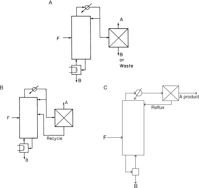
FIGURE 8-1. Breaking azeotropes; (A) separator uncoupled with distillation, (B) recycle from separator to distillation, (C) separator produces reflux for distillation column
The most common configuration is that of Figure 8-1B. The incompletely separated stream is recycled to the distillation column, which now operates as a two-feed column, so the design procedures used for two-feed columns (Example 4-5) can be used. The arrangement shown in Figure 8-1B is commonly used industrially. The separator may actually be several separators.
In the third configuration the separator produces one product and the reflux for the distillation column (Figure 8-1C). This arrangement is used for heterogeneous azeotropes in the next section.
8.2 Binary Heterogeneous Azeotropic Distillation Processes
The presence of an azeotrope can be used to separate an azeotropic system. This is most convenient if the azeotrope is heterogeneous; that is, the vapor from the azeotrope will condense to form two liquid phases that are partially immiscible. Azeotropic distillation is often performed by adding a solvent or an entrainer that forms an azeotrope with one or both of the components. Before discussing these more complex azeotropic distillation systems in Section 8.7, we explore simpler binary systems that form heterogeneous azeotropes.
8.2.1 Binary Heterogeneous Azeotropes—Single-Column System
Although not common, there are systems such as n-butanol and water that form a heterogeneous azeotrope (Figure 8-2). Figures 8-2A and 8-2B plot the same data but for different components. You should feel comfortable converting from Figure 8-2A to 8-2B and vice versa. Both graphs show that when vapor of the azeotrope with mole fraction yaz is condensed, a water-rich liquid phase, α, and an organic-rich liquid phase, β, separate from each other.
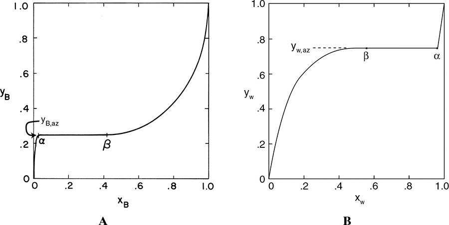
FIGURE 8-2. Heterogeneous azeotrope system, n-butanol and water at 1.0 atm (Chu et al., 1950). (A) Plotted as butanol mole fractions. (B) Plotted as water mole fractions
How should we distill a feed that forms a heterogeneous azeotrope? Suppose we have a saturated liquid feed that is 40.0 mol% water and 60.0 mol% n-butanol. The distillation system shown in Figure 8-3A (Luyben, 1973) consists of a column and a liquid-liquid settler. The column will produce a pure butanol product as the bottoms. The distillate product is the aqueous layer from the settler and automatically has xw,dist = xw,α. We can develop the top operating line using the mass balance envelope shown in Figure 8-3A.
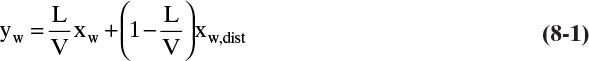
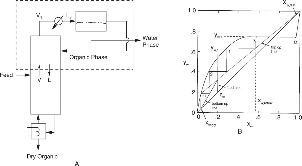
FIGURE 8-3. Distillation column plus settler for distillation of system with heterogeneous azeotrope. (A) One-column system. (B) McCabe-Thiele diagram
This looks like a normal top operating equation, but there will be differences in the way it is plotted and the way it is used. The bottom operating equation looks normal and when plotted gives the normal bottom operating line.
Since the distillation column operates in the concentration region where water is the more volatile component (MVC), the McCabe-Thiele diagram will look normal if we use Figure 8-2B. The top operating line has slope = L/V, ![]() , and y = x intersection of y = x = xw,dist (Figure 8-3B). Note that xw,dist = xw,α, and the top operating line goes through y = x = xw,dist not the equilibrium curve at xw,α. The top operating line cuts through the equilibrium curve, which may seem impossible, but the distillation does not operate in this range. Instead the separation from xw,α to xw,β is done in a liquid-liquid separator or decanter. Reflux in Figures 8-3A and 8-3B has a mole fraction of xw,reflux = xw,β, not the distillate composition. In the column, xw,reflux and yw,1 are passing steams and are on the operating line in Figure 8-3B. Stepping off remaining stages follows the normal procedure.
, and y = x intersection of y = x = xw,dist (Figure 8-3B). Note that xw,dist = xw,α, and the top operating line goes through y = x = xw,dist not the equilibrium curve at xw,α. The top operating line cuts through the equilibrium curve, which may seem impossible, but the distillation does not operate in this range. Instead the separation from xw,α to xw,β is done in a liquid-liquid separator or decanter. Reflux in Figures 8-3A and 8-3B has a mole fraction of xw,reflux = xw,β, not the distillate composition. In the column, xw,reflux and yw,1 are passing steams and are on the operating line in Figure 8-3B. Stepping off remaining stages follows the normal procedure.
The vapor of mole fraction yw,1 is condensed and sent to the decanter. The mass balances for the decanter are straightforward and illustrated in Example 8-1.
What can we do if we want a purer water product?
8.2.2 Binary Heterogeneous Azeotropes—Two-Column System
For this heterogeneous azeotrope the two-column system shown in Figure 8-4A can do a complete separation. The first column, which is a complete column since it receives a feed stream and has both rectifying and stripping sections, operates on the left-hand side of Figure 8-3B, where water is the MVC. Thus, the bottoms from this column is almost pure n-butanol (xw,bot,complete ∼ 0). Column 2 is a stripping column that receives liquid of composition xα from the liquid-liquid separator. It operates where n-butanol is more volatile (low n-butanol mole fractions on Figure 8-2A) and bottoms from column 2 is almost pure water (xbutanol,bot,strip ∼ 0).

FIGURE 8-4. Binary heterogeneous azeotrope separation on n-butanol, B, and water, W; (A) two-column distillation system, (B) McCabe-Thiele diagram for column 1, (C) McCabe-Thiele diagram for column 2 with expanded coordinates
Overhead vapor from both columns is condensed and sent to the decanter. This separator takes the two condensed liquids, xα < x < xβ, and separates them into two liquid phases in equilibrium at mole fractions xα and xβ. These liquids are refluxed to the stripping and complete columns, respectively. The decanter fulfills the role of the separator shown in Figure 8-1C.
The overall external mass balance for the two-column system shown in Figure 8-4A is
while the external mass balance on water is
Solving these equations simultaneously for the unknown bottoms flow rates, we obtain

Note that Eqs. (8-4) and (8-5) do not depend on the details of the distillation system.
The bottom operating equation for the complete column is Eq. (8-2). The top operating line is a bit different. The easiest mass balance to write uses the mass balance envelope shown in Figure 8-4A. The top operating equation for the complete column is
This is somewhat unusual because it includes a bottoms concentration leaving the stripping column (column 2). The reflux for this top operating line is liquid of composition xw,β. The McCabe-Thiele diagram for this system is shown in Figure 8-4B and is almost identical to Figure 8-3B.
Analysis of stripping column 2 is straightforward. It is easiest to use Figure 8-2A and develop the operating equation for n-butanol. This bottom operating equation is

The feed to this column is the saturated liquid reflux of composition xbutanol,α, which is represented by a vertical feed line. Then the overhead vapor yB,strip is found on the operating line at xB,α (Figure 8-4C).
Note that column 1 operates in a region where water is most volatile, and column 2 operates where n-butanol is more volatile. McCabe-Thiele diagrams are most familiar and hence easiest to use if plotted for the MVC. Thus, we plotted water mole fractions for column 1 and n-butanol mole fractions for column 2. It is also possible to do the calculations on a single diagram (Wankat, 2007), which results in one of the calculations looking upside down.
The operation of distillation columns separating heterogeneous azeotropes can be quite erratic (Kovach and Seider, 1987). Small shifts in the aqueous reflux rate can cause a number of trays to shift from operation in a homogeneous region to a heterogeneous region. This erratic switching causes large variations in product purity. These columns need very careful control of reflux flow rate to operate properly.
Several modifications of the basic arrangement shown in Figure 8-4A can be used. If the feed composition is less than xbutanol,α, column 2 becomes a complete column and column 1 a stripping column. Liquids from the condensers may be subcooled since the partial miscibility of many systems depends on temperature. If liquids are subcooled, separator calculations must be done at the separator temperature. Then reflux concentrations can be plotted on the McCabe-Thiele diagram. Design of separators (decanters) is discussed in Section 13.14.2. Heterogeneous azeotropes are explored in depth by Doherty et al. (2008), Doherty and Malone (2001), and Shinskey (1984).
Unfortunately, the presence of a second liquid phase tends to make problem solution confusing. The following comments may help clarify the procedure:
• Label mole fractions, columns, and streams clearly.
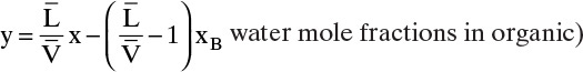
• The organic product (n-butanol in this example) is recovered as the bottoms from the organic column operating with a liquid organic phase; however, we plot water mole fractions on the McCabe-Thiele diagram (because water is the MVC when it is dissolved in organic).
• The water product is recovered from the water column operating with a liquid aqueous phase; however, we plot organic mole fractions on the McCabe-Thiele diagram (because organic is the MVC when it is dissolved in water).
• Sketch the flowsheet. The flow sheet will depend on the concentration(s) of the feed(s). For example, if the feed is a vapor with a concentration between β and α on Figure 8-4B, it should be fed to one of the condensers, and both columns will be strippers (see Problem 8.D5).
• The operating equations depend on the equipment layout. Draw mass balance envelopes on your flowsheet, and derive the operating equations.
Once you become skilled at solving heterogeneous azeotrope problems with McCabe-Thiele diagrams, you will have mastered the use of McCabe-Thiele diagrams for binary distillation. Study Example 8-1 in the next section, and practice solving problems.
8.2.3 Drying Organic Compounds That Are Partially Miscible with Water
For immiscible systems (really partially miscible systems) of organics and water, a single phase is formed only when the water concentration is low or very high. For example, a small amount of water can dissolve in gasoline. If more water is present, two phases will form. In the case of gasoline, the water phase is detrimental to the engine and in cold climates can freeze in gas lines, immobilizing the car. Since the solubility of water in gasoline decreases as the temperature is reduced, it is important to have dry gasoline.
Fortunately, small amounts of water can easily be removed by distillation or adsorption (Chapter 18). During distillation the water acts as a very volatile component, so a mixture of water and organics is taken as the distillate. After condensation, two liquid phases form, and the organic phase can be refluxed. The system is a type of heterogeneous azeotropic system essentially identical to Figure 8-3A. The water product is usually sent to waste treatment. With very high relative volatilities, one equilibrium stage may be sufficient, and a flash system plus a separator can be used. The only new material in this section is the theory for equilibrium of dilute immiscible phases.
Because detailed equilibrium data are often unavailable, simplified equilibrium theories are useful for immiscible liquids. There is always a range of concentrations where the species are miscible even though the concentrations may be quite small. It is reasonable to assume that the relative volatility is constant over the small range of compositions where the liquids are miscible. The relative volatility is defined as
If data for the heterogeneous azeotrope (yw,az and xw,az in org) are available, then
and the relative volatility can be calculated from
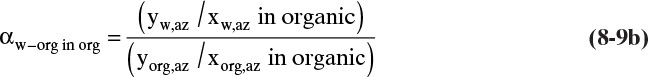
Using azeotrope data to calculate a relative volatility is more accurate than assuming Raoult’s law or assuming a linear relationship.
If azeotropic data are not available, we can assume for the water phase that water follows Raoult’s law and organic components follow Henry’s law (Robinson and Gilliland, 1950). Thus,
where Horg is the Henry’s law constant for the organic component in the aqueous phase, VPw is the vapor pressure of water, pw and porg are the partial pressures of water and organic, and xw_in_w and xorg_in_w are the mole fractions of water and organic in the water phase, respectively. In the organic phase, it is reasonable to use Raoult’s law for the concentrated organic compounds and Henry’s law for the water, which is very dilute.
where Hw is the Henry’s law constant for water in the organic phase. At equilibrium, the partial pressure of water in the two phases must be equal. Thus, equating pw in Eqs. (8-10a) and (8-10b) and solving for Hw we obtain

Similar manipulations for the organic component in water give

Using Eqs. (8-11a) and (8-11b), we can determine the Henry’s law constants from the known solubilities (which give the mole fractions) and the vapor pressures.
Equations (8-8) to (8-11) are valid for both drying organic compounds and steam distillation (Section 8.3). The ease of removing small amounts of water from an organic compound that is immiscible with water can be seen by estimating the relative volatility of water in the organic phase.

In the organic phase Eqs. (8-10b) and (8-11b) can be substituted in Eq. (8-12) to give

This calculation is illustrated in Example 8-1 where the estimate is αw–benzene_in_org = 31.3.
Organics can be dried either by continuous distillation or by batch distillation. In both cases the vapor condenses into two phases. The water phase can be withdrawn and the organic phase refluxed to the distillation system. For continuous systems, the McCabe-Thiele design procedure can be used. The McCabe-Thiele equilibrium can be plotted with the relative volatility calculated from Eq. (8-9b) or (8-13), and the analysis is the same as in the previous section. This is illustrated in Example 8-1.
EXAMPLE 8-1. Drying benzene by distillation
A benzene stream contains 1.0 mol% water. The flow rate is 100.0 kmol/h, and the feed is a saturated liquid. The column has saturated liquid reflux of the organic phase from the liquid-liquid separator (see Figure 8-3A) and uses L/D = 2.0(L/D)min. We want the outlet benzene to have xw_in_benz,bot = 0.001. Because of the small changes in mole fractions in the column, CMO is a reasonable assumption. Design the column and the liquid-liquid separator.
Solution
A. Define. The column is the same as Figure 8-3A. Find the total number of stages and the optimum feed stage. For the separator determine the compositions and flow rates of the water and organic phases.
B. Explore. Need equilibrium data. Robinson and Gilliland (1950) give the following solubility data: xbenz_in_w,α = 0.00039 and xw-in_benz,β = 0.015. The solubility data, which are also the azeotropic data, give the compositions of the streams leaving the settler. Use Eq. (8-13) for equilibrium. At the boiling point of benzene (80.1°C), VPbenz = 760.0 mm Hg, and VPw = 356.6 mm Hg (Perry and Green, 1997). Operation will be at a different temperature, but the ratio of vapor pressures will be approximately constant.
C. Plan. Calculate equilibrium from Eq. (8-13):
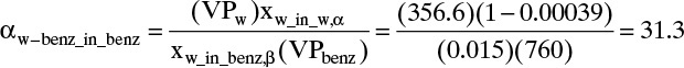
This is a good approximation of VLE for xw_in_benz < 0.015. After that, we have a heterogeneous azeotrope. Plot the curve represented by this value of αw-benz_in_benz on a McCabe-Thiele diagram. (Two diagrams will be used for accuracy.) Solve with the McCabe-Thiele method as a heterogeneous azeotrope problem. Mass balances will be used to find flow rates leaving the settler.
B. Do it. Plot equilibrium: ![]() (organic phase)
(organic phase)
This equation is valid for xw_in_org ≤ 0.015. At the solubility limit (the heterogeneous azeotrope) xw_in_org,β = 0.015, we can determine the yw value for the azeotrope:

See Figure 8-5. Since Figure 8-5A is obviously not accurate for stepping off stages, we use expanded Figure 8-5B. Calculate the vapor mole fraction in equilibrium with the feed, (L/V)min, (L/D)min, (L/D)actual, and (L/V)actual. From equilibrium
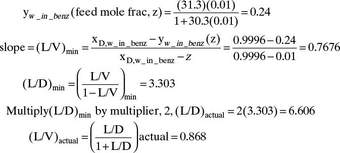
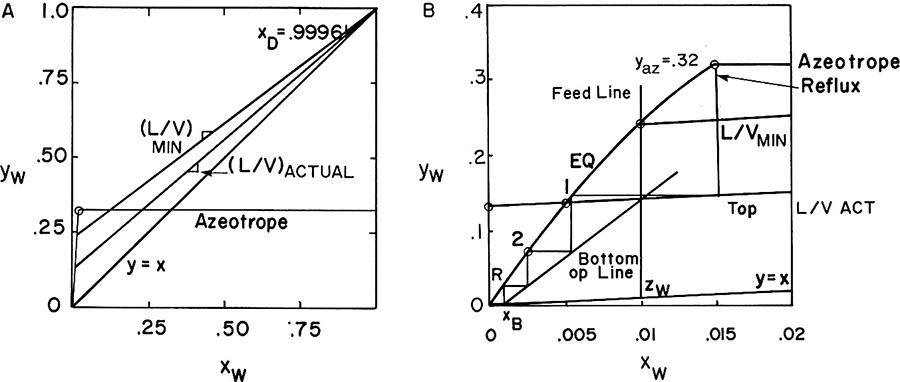
FIGURE 8-5. Solution for Example 8-1; (A) McCabe-Thiele diagram for entire range, (B) McCabe-Thiele diagram for low concentrations
Top Operating Line: (y and x are mole fractions of MVC, water, in organic)
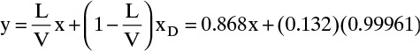
where xD is the water mole fraction in the distillate. Since the distillate is water saturated with benzene, xD = 1 – xbenz in w,α = 1 – 0.00039 = 0.99961.
y intercept (x = 0) = 0.132
y = x = xD = 0.99961
Plot the top operating line (Figure 8-5A).
Bottom Operating Line:
goes through y = x = xB = 0.001 and the intersection of the top operating line and the feed line.
Reflux is the benzene phase from the liquid-liquid separator (see Figure 8-3A); thus, xreflux = xw in benz,β = 0.015. Start stepping off stages on Figure 8-5B with returned reflux. The optimum feed stage is the top stage of the column. We need two stages and a partial reboiler.
External mass balances: From Eq. (3-3):

B = F – D = 100.0 – 0.901 = 99.099 kmol/h
Separator Mass Balances: Organic phase leaves the settler as reflux (stream L) to the distillation column.
L = (L/D)D = 6.606 D = 5.954 (Organic phase)
The vapor leaving stage 1, y1,w, is a passing stream to the reflux and satisfies the mass balance used to derive the top operating line.
y1,w = (0.868)(0.015) + (0.132)(0.99961) = 0.145
Stream V1 is condensed and enters the separator as a two-phase liquid mixture with average mole fraction xw,L_in = yw,V1 = 0.145 and flow rate Lin, which settles into the organic and the aqueous liquid layers in the settler.
V1 = Lin = L + D = 6.855, and Lin xw,L_in = L xw,reflux,in_benzene + D xD,w
Since Lin and the mole fractions are known, we can solve for the flow rates of the organic L and aqueous D phases leaving the settler.

Results are ![]() and
and
L = Lin – D = 6.855 – 0.908 = 5.947 kmol/h
E. Check. All internal consistency checks work. The value of αw–benz_in_benz agrees with the calculation of Robinson and Gilliland (1950). The best check on αw–benz_in_benz is comparison with a value calculated from Eq. (8-9b) with experimental data for yw,az. This value is reported as yw,az = 0.298 in the Dortmund Data book (DDBST, 2016), and the resulting value of αw–benz_in_benz = 27.87. Although the approximate calculation is off, the basic conclusion that water is easy to distil from benzene is correct. In addition, comparison of the settler flow rates with results from external mass balances were in agreement.
F. Generalize. Since the solubility of organics in water is often very low, this type of heterogeneous azeotrope system requires only one distillation column.
Even though water has a higher boiling point than benzene, the relative volatility of water dissolved in benzene is extremely high. This occurs because water dissolved in an organic cannot hydrogen bond as it does in an aqueous phase, and thus, it acts as a very small molecule that is quite volatile. One practical consequence of this is that small amounts of water can easily be removed from organics if the liquids are partially immiscible. However, there are alternative methods for drying organics such as adsorption that may be cheaper than distillation in many cases.
8.3 Steam Distillation
In steam distillation, water (as steam) is intentionally added to a distilling organic mixture to reduce the required temperature and to keep suspended any solids that may be present. Steam distillation may be operated with one or two liquid phases in the column. In both cases overhead vapor condenses into two phases. Thus, the system can be considered a type of azeotropic distillation in which the added solvent is water and the separation is between volatiles and nonvolatiles. This is a pseudo-binary distillation with water and the volatile organic forming a heterogeneous azeotrope. Steam distillation is commonly used for purification of essential oils in the perfume industry, for distillation of organics obtained from coal, for hydrocarbon distillations, and for removing solvents from solids in waste disposal (Ludwig, 1997).
For steam distillation with a liquid water phase present, the equilibrium law is, both the water and organic layers exert their own vapor pressures. At 1.0 atm pressure the temperature must be less than 100.0°C even though the volatile organic material by itself might boil at several hundred degrees. Thus, one advantage of steam distillation is lower operating temperatures. With two liquid phases present and in equilibrium, their compositions are fixed by their mutual solubilities. Since each phase exerts its own vapor pressure, vapor composition is constant regardless of average liquid concentration. A heterogeneous azeotrope is formed. As the amount of water or organic is increased, phase concentrations do not change—only the amount of each liquid phase changes. Since an azeotrope has been reached, no additional separation is obtained by adding more stages. Thus, only a reboiler is required. Steam distillation is often a batch operation (see Chapter 9).
Equilibrium calculations are similar to those for drying organics, except that now two liquid phases are present. Since each phase exerts its own vapor pressure, the total pressure is the sum of the partial pressure of the volatile organic from the organic phase and the partial pressure of the water from the aqueous phase. With one volatile organic
Substituting in Eqs. (8-10a) and (8-10b), we obtain
Compositions of liquid phases are set by equilibrium. If the total pressure is fixed, Eq. (8-15b) enables us to calculate the temperature. Once the temperature is known the vapor composition is calculated as

If several organics are present, yorg and porg are the sums of the respective values for all the organics. If we assume that the water and organic phases are completely immiscible, then xw in w = 1.0.
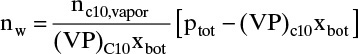
The number of moles of water carried over in the vapor can be estimated, since the ratio of moles of water to moles of organic is equal to the ratio of vapor mole fractions.

Substituting in Eq. (8-16), we obtain

The total moles of steam required are nw plus the moles condensed to heat and vaporize the organic (see Example 8-2).
EXAMPLE 8-2. Steam distillation
Cutting oil that has approximately the properties of n-decane (C10 H22) is to be recovered from nonvolatile oils and solids in a steady-state, single-stage steam distillation. Operation will be with liquid water present. The feed is 50.0 mol% n-decane and 50.0 mol% nonvolatile organics. A bottoms that is 15.0 mol% n-decane in the organic phase is desired. The feed rate is 10.0 kmol/h. The feed enters at the boiler’s temperature. Pressure is barometric, which in your plant is approximately 745 mm Hg. Find:
A. The temperature of the still.
B. The moles of water carried over in the vapor.
C. The moles of water in the bottoms.
Solution
A. Define. The still is sketched in the figure. Note that there is no reflux.
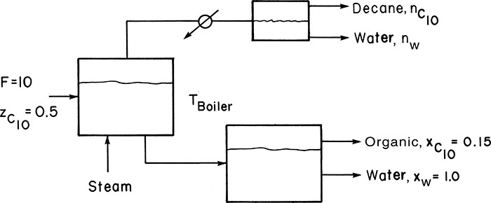
B. Explore. Equilibrium is given by Eq. (8-16). Assuming the organic and water phases are completely immiscible, we have in the bottoms xC10 in org = 0.15, xw in w = 1.0 and in the two distillate layers xC10,org,dist = 1.0 and xw,water,dist = 1.0.Vapor pressure data are available in Perry and Green (1997). Then Eq. (8-15b) can be solved by trial and error to find Tboiler. Equation (8-18) and a mass balance can be used to determine the moles of water and decane vaporized. The moles of water condensed to vaporize the decane can be determined from an energy balance. Latent heat data are available in Perry and Green (1997).
C. Plan. On a water-free basis the mass balances around the boiler are
where B is the molar flow rate of the organic phase in the bottoms, and nC10,vapor is the molar flow rate of C10 in the vapor. Since F = 10.0, xbot = 0.15, and zC10 = 0.5, we can solve for nC10,vapor and B. Eq. (8-18) gives nw once Tboiler is known. Since feed, bottoms, and vapor are all at Tboiler, the energy balance simplifies to
nC10λC10 = (moles of water condensed in still)λw
D. Do it.
a. Perry and Green (1997) give the following n-decane vapor pressure data (vapor pressure in mm Hg and T in °C):
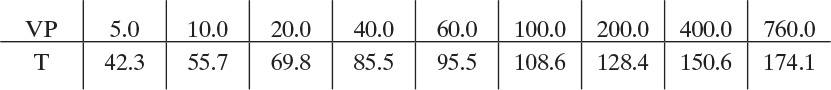
A complete table of water vapor pressures is available (see Problem 8.D10). As a first guess, try 95.5°C, where (VP)w = 645.7 mm Hg. Then Eq. (8-15),
(VP)C10 xC10 in org + (VP)w xw in w = ptot
For completely immiscible phases Eq. (8-15) becomes
(60.0)(0.15) + (645.7)(1.0) = 654.7 < 745 = ptot
This temperature is too low. Approximate solution of Eq. (8-15) eventually gives Tboiler = 99.0°C and (VP)C10 = 66.0 mm Hg.
b. Solving the mass balances, Eqs. (8-19), kmol/h of vapor is
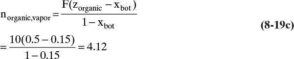
which is 586.2 kg/h. Eq. (8-18),
is

c. The moles of water required to vaporize the decane is found by
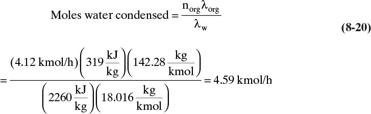
where λ = Hvap – hliq, and the saturated vapor and liquid enthalpies at 99.0°C are interpolated from Tables 2-249 and 2-352 in Perry and Green (1997) for decane and water, respectively.
E. Check. A check for complete immiscibility is advisable since all the calculations are based on this assumption.
F. Generalize. Obviously, the decane is boiled over at a temperature well below its boiling point, but a large amount of water is required. Most of this water is carried over in the vapor. On a weight basis, the kilograms of total water required per kilogram decane vaporized are 9.26. Less water will be used if the boiler is at a higher temperature and there is no liquid water in the still. Less water is also used for higher values of xorg,bot (see Problem 8.D10).
Additional separation can be obtained by operating without a liquid water phase in the column. Reducing the number of phases increases the degrees of freedom by one. Operation must be at a temperature higher than that predicted by Eq. (8-15), or a liquid water layer will form in the column. Thus, the column must be heated with a conventional reboiler and/or the sensible heat available in superheated steam. The latent heat available in the steam cannot be used because it would produce a layer of liquid water. Operation without liquid water in the column reduces the energy requirements but makes the system more complex.
8.4 Pressure-Swing Distillation Processes
Pressure affects vapor-liquid equilibrium (VLE), and in systems that form azeotropes, it affects azeotrope composition. For example, Table 2-1 shows ethanol-water has an azeotrope at 89.43 mol% ethanol at 1.0 atm pressure. If pressure is reduced, azeotropic concentration increases (Seader, 1984). At pressures below 70.0 mm Hg, the azeotrope disappears entirely, and distillation can be done in a simple column. Unfortunately, separation of ethanol and water at pressures below 70 mm Hg is not economical because the column requires a large number of stages and a large diameter (Black, 1980). However, the principle of finding pressures at which azeotropes disappear may be useful for other distillations. The effect of pressure on azeotropic composition and temperature can be estimated using VLE correlations in process simulators (Wasylkiewicz, 2006).
Azeotropes do not have to disappear for concentration shifts with pressure to be useful. If the composition shift is large enough, the two-column distillation at two different pressures shown in Figure 8-6 can completely separate binary mixtures (Doherty and Malone, 2001; Drew, 1997; Frank, 1997; Mahdi et al., 2015; Shinskey, 1984; Van Winkle, 1967). Doherty et al. (2008) recommend a minimum mole fraction change of 5.0% (e.g., from 55.0% to 60.0%) with a 10.0% change being preferable. Column 1 usually operates at atmospheric pressure, while column 2 is usually at a higher pressure but can be at a lower pressure.
To understand the operation of this process, consider separation of methyl ethyl ketone (MEK) and water (Drew, 1997). At 1.0 atm the azeotrope contains 35.0% water, while at 100.0 psia the azeotrope is 50.0% water. If a feed containing more than 35.0% water is fed to the first column in Figure 8-6, the bottoms will be pure water. Distillate from this atmospheric column will be the 35.0% azeotrope. When this azeotrope is sent to the high-pressure column, an azeotrope containing 50.0% water comes off as the distillate; this distillate is recycled to column 1. Since the feed to column 2 (the 35.0% azeotrope) contains less water than the distillate, the bottoms from column 2 is pure MEK. Note that water is less volatile in column 1, and MEK is less volatile in column 2.
The external mass balances for Figure 8-6 are identical to Eqs. (8-3a) and (8-3b). Thus, the bottoms flow rates are given by Eqs. (8-4) and (8-5). Although the processes shown in Figures 8-4A and 8-6 are very different, they look the same to the external mass balances. Process differences become evident when balances are written for individual columns. For instance, for column 2
and
Solving these equations simultaneously and then inserting the results in Eq. (8-4b), we obtain

As the two azeotrope concentrations at the two different pressures approach each other, xdist1 – xdist2 becomes small. According to Eq. (8-23), the recycle flow rate D2 becomes large. This increases both operating and capital costs and makes this process expensive.
The two-pressure system is used for the separation of acetonitrile-water, tetrahydrofuran-water, methanol-MEK, and methanol-acetone (Frank, 1997). In the latter application the second column is at 200 torr. Mahdi et al. (2015) review the recent studies of pressure-swing distillation. Realize that these applications are rare. For most azeotropic systems, the shift in the azeotrope with pressure is small, and use of the system shown in Figure 8-6 involves a very large recycle stream. This causes the first column to be large, and costs become excessive.
Before the relatively recent development of detailed and accurate VLE correlations, most VLE data were only available at 1.0 atm; thus, many azeotropic systems have probably not been explored as candidates for two-pressure distillation. Currently, it is fairly easy to simulate pressure-swing distillation with a process simulator (see Lab 7 in this chapter’s appendix). Methods for estimating VLE and rapidly screening possible systems are available (Frank, 1997). Because two-pressure distillation does not require a mass separating agent, it is a preferred method when it works. If two-pressure distillation were routinely considered as an option for breaking azeotropes, we would undoubtedly discover additional systems in which this method is economical.
8.5 Complex Ternary Distillation Systems
In Chapters 5 to 7 we studied multicomponent distillation for systems with relatively ideal VLE that do not exhibit azeotropic behavior. In Chapter 4 when we studied both relatively ideal and azeotropic binary systems we found that there were significant differences between these systems. If no azeotrope forms, you can obtain essentially pure distillate and pure bottoms products. If there is an azeotrope, you can at best obtain one pure product and the azeotrope. If the binary azeotrope is heterogeneous, you can usually use a liquid-liquid separator to get past the azeotrope and obtain two pure products with two columns (Section 8.2). Ternary systems with nonideal VLE can have one or more azeotropes that may be homogeneous or heterogeneous. Since behavior of ideal ternary distillation is more complex than that of ideal binary distillation, we expect that behavior of nonideal ternary distillation is probably more complex than nonideal binary distillation.
Although McCabe-Thiele diagrams can be used for ternary systems, they have not been nearly as successful as binary applications. Hengstebeck (1961) developed a pseudo-binary approach that is useful for systems with close to ideal VLE. It has also been applied to extractive distillation by assuming solvent concentration is constant. Chambers (1951) developed a method that could be applied with fewer assumptions to systems with azeotropes and illustrated it with the ternary system methanol-ethanol-water. His approach consists of drawing two McCabe-Thiele diagrams (e.g., one for methanol and one for ethanol). Equilibrium consists of several curves with the methanol mole fraction as a parameter on the ethanol diagram and the ethanol mole fraction as a parameter on the methanol diagram. Each equilibrium step required simultaneous solution of the two diagrams. The operating lines plot on these diagrams in the normal fashion. Although visually instructive, Chambers’ method is awkward and has not been widely used. The conclusion is we need new visualization tools to study ternary distillation.
8.5.1 Distillation Curves
You may have noticed in Chapter 2 that enthalpy-composition and temperature-composition diagrams contain more information than McCabe-Thiele y-x diagrams. We started using diagrams with less information because it was easier to show patterns and visualize the separation. For ternary distillation we repeat this pattern and go to a ternary composition diagram that shows the paths taken by liquid mole fractions throughout a distillation operation. We gain in visualization power, since a variety of possible paths is easy to illustrate, but we lose power since the stages are no longer shown. For complex systems the gains are much more important than the losses.
A distillation curve is a plot of mole fractions on every tray for distillation. Distillation curves can be generated at total or finite reflux. If you have run a multicomponent distillation simulation or solved a ternary distillation problem with a hand calculation, you have obtained the information (xi,j for j = 1, ... N) necessary to plot a distillation curve. Thus, the difference is the presentation. Two different formats used for these diagrams are shown in Figures 8-7 and 8-8. To generate these plots at total reflux, consider a distillation column numbered from the bottom up (Figure 5-1). If we start at the reboiler, we first do a bubble-point calculation:

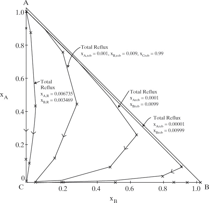
FIGURE 8-7. Distillation curves at total reflux for constant relative volatility system; A = benzene, B = toluene, C = cumene; αAB = 2.4, αBB = 1.0, and αCB = 0.21; stages are shown as ×
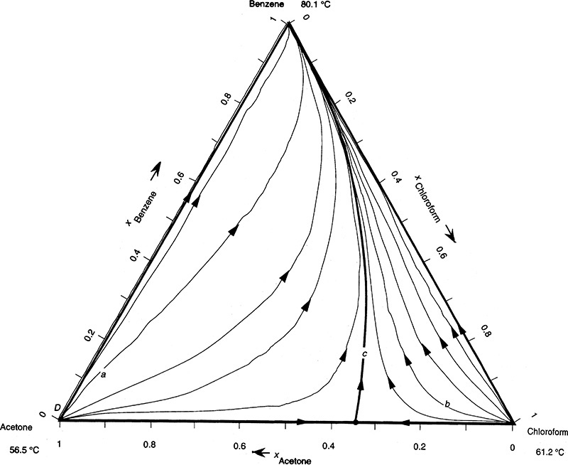
FIGURE 8-8. Distillation curves at total reflux for acetone, chloroform, and benzene mixtures at 1.0 atm (Biegler et al., 1997), reprinted with permission of Prentice-Hall PTR, copyright 1997, Prentice-Hall.
Calculation of the bubble point at every stage can be laborious; fortunately, the calculation is easily done with a process simulator. Next, at total reflux the operating equation is
Alternation of these two equations results in values for xA, xB, and xC on every stage. These values (see Example 8-3) are then plotted in Figures 8-7 and 8-8. The starting mole fractions are chosen so that distillation curves fill the entire space of the diagrams.
If the relative volatility is constant, then the vapor mole fractions can be easily calculated from Eq. (5-28) (in Problem 5.C1). Substituting Eq. (5-28) in Eq. (8-25a) and solving for xi,j+1, we obtain a recursion relationship for generating a distillation curve for constant relative volatility systems.
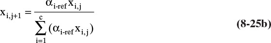
Figure 8-7 shows the characteristic pattern of distillation curves for ideal or close to ideal VLE with no azeotropes. All systems considered in Chapters 5, 6, and 7 follow this pattern. The y-axis (xB = 0) represents the binary A-C separation. This starts at the reboiler (xA = 0.01 is an arbitrary value) and requires only the reboiler plus four stages to reach a distillate value of xA = 0.994. The x axis (xA = 0) represents the binary B-C separation, which was started at the arbitrary value xB = 0.01 in the reboiler. The maximum in B concentration should be familiar from the profiles shown in Chapter 5. Distillation curves at finite reflux ratios are similar but not identical to those at total reflux. Note that the entire space of the diagram can be reached by starting with concentrations near 100.0% C (the heavy boiler). Distillation curves are usually plotted as smooth curves—they were plotted as discrete points in this diagram to emphasize the location of the stages. Arrows are traditionally shown in the direction of increasing temperature. Your understanding of the procedure for plotting these curves will be aided significantly by studying Example 8-3 and doing Problem 8.H1.
Figure 8-8 (Biegler et al., 1997) shows total reflux distillation curves for acetone, chloroform, and benzene distillation on an equilateral triangle diagram. This system has a maximum boiling azeotrope between acetone (xacetone ∼ 0.34) and chloroform. To reach compositions on the right side of the diagram we need to start with locations that are to the right of distillation boundary curve c. For compositions on the left side of the diagram we have to start with locations that are to the left of the distillation boundary. For a given feed concentration, only part of the space in Figure 8-8 can be reached for distillate and bottoms products. If we want to produce pure acetone in a single column, the feed needs to be to the left of the distillation boundary. To produce pure chloroform, the feed needs to be to the right of the distillation boundary. Although the distillation boundary will move slightly at finite reflux ratios, this basic principle still holds. Figure 8-8 is unusual because it shows a relatively rare maximum boiling azeotrope. All of the other systems we consider are the much more common minimum-boiling azeotropes.
We can do mass balances on triangular diagrams. First, consider separation of binaries, which occur along the y-axis, the x-axis, and the hypotenuse of the right triangle. In Figure 8-9 the binary separation of the heavy (highest boiling) component, H, from the intermediate component, I, occurs along the y-axis (line B1F1D1).
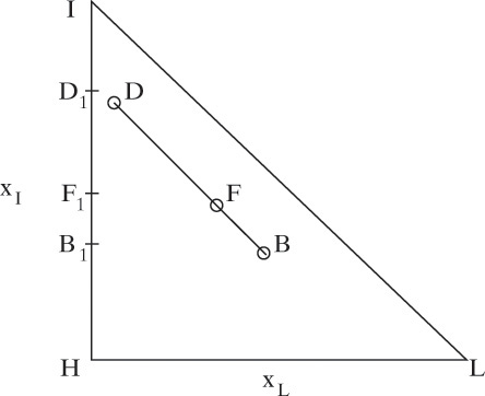
In Chapter 3 we developed Eq. (3-3) for binary separations. This equation applies to each component in multicomponent separations. For example, for separation of intermediate and heavy components,

Equation (8-26) remains valid if a third (or fourth or more) component is present, and we can write a similar equation for each component. Thus, Eq. (8-26) applies for the general ternary separation shown as line BFD. This equation also proves that the points representing bottoms, distillate, and the feed all lie on a straight line and that the lever-arm rule applies. (Rules for mass balances on triangular diagrams are developed in detail in Section 13.8.) As a first approximation, the points representing bottoms and distillate products from a distillation column with a single feed will lie on the distillation and residue curves (see next section). The path traced from distillate to bottoms must follow the same direction as the arrows (increasing temperature). Thus, these curves will show us if the separation indicated by the line BFD is feasible. If there is a distillation boundary as in Figure 8-8, not all separations will be feasible.
8.5.2 Residue Curves
We could do all of our calculations with distillation curves at total and finite reflux ratios; however, these curves depend to some extent on the distillation system. It is convenient to use a thermodynamically based curve that does not depend on the number of stages. A residue curve is generated by putting a mixture in a still pot and boiling it without reflux until the pot runs dry and only the residue remains (Doherty and Malone, 2001; Skiborowski et al., 2014). This is a simple batch distillation that is discussed in more detail in Chapter 9. The plot of changing mole fractions on a triangular diagram is called a residue curve. It will be similar but not identical to the distillation curves shown in Figures 8-7 and 8-8. The differences are explored by Widagdo and Seider (1996).
A simple equilibrium still is shown in Figure 8-10. As distillation continues, molar holdup of liquid H in the still decreases. The unsteady-state overall mass balance is
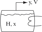
where V is the molar rate (not necessarily constant) at which vapor is removed. Component mass balances have a similar form:

Expanding the derivative, substituting in Eq. (8-27a), and rearranging, we obtain

This derivation closely follows the derivations in Biegler et al. (1997) and Doherty and Malone (2001). An alternate derivation is given in Sections 9.1 and 9.2.
Integration of Eq. (8-27c) gives values of xi versus time and allows us to plot the residue curve. This integration can be done with any suitable numerical integration technique; however, the vapor mole fraction y in equilibrium with x must be determined at each time step. Although Doherty and Malone (2001) recommend the use of either Gear’s method or a fourth-order Runge-Kutta integration, they note that Eq. (8-27c) is well behaved and can be integrated with Euler’s method. This method is particularly simple. Write Eq. (8-27c) as a difference equation.

Define h as
Then at the next step
where k refers to the step number and h is the step size. A constant step size of h = 0.01 or smaller is recommended (Doherty and Malone, 2001).
In general, bubble-point calculations are required for each step (see Problem 8.H3); however, if relative volatilities are constant, we can determine y from Eq. (5-28) (in Problem 5.C1), and the recursion relationship simplifies to

Despite the fact that process simulators do these calculations for us, doing the integration for a simple case will greatly increase your understanding. Thus, studying Example 8-3 and doing Problem 8.H2 are highly recommended.
Siirola and Barnicki (1997) and Doherty et al. (2008) show simplified residue curve plots for all 125 possible systems. The most common residue curve is the ideal distillation plot, which is similar to Figure 8-7. Next most common are systems with a single minimum-boiling azeotrope occurring between one of the binary pairs. The three possibilities are shown in Figure 8-11 (Doherty and Malone, 2001). As mentioned earlier, a residue curve plot for a maximum boiling azeotrope as shown in Figure 8-8 is rare. You can also have multiple binary and ternary azeotropes (Doherty et al., 2008; Siirola and Barnecki, 1997). Heterogeneous ternary azeotropes can also occur and are important in azeotropic distillation (Doherty and Malone, 2001; Skiborowski et al., 2014). Figure 8-12 (Doherty and Malone, 2001) is an example of the residue curves that occur in azeotropic distillation with added solvent. The systems shown in Figures 8-11C and 8-12 are often formed on purpose by adding a solvent to a binary azeotropic system.

FIGURE 8-11. Schematics of residue curve maps when there is one binary minimum-boiling azeotrope (Doherty and Malone, 2001); reprinted with permission of McGraw-Hill, copyright 2001, McGraw-Hill
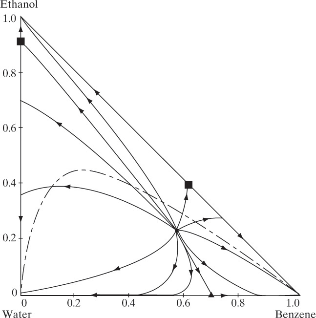
FIGURE 8-12. Calculated residue curve map for ethanol-water-benzene (Doherty and Malone, 2001). The black squares are binary homogeneous azeotropes, the black triangle is a heterogeneous binary azeotrope, the black dot in the center of the diagram is a heterogeneous ternary azeotrope, and the dot-dash line represents the solubility envelope for the two liquid layers. Reprinted with permission of McGraw-Hill, copyright 2001, McGraw-Hill
EXAMPLE 8-3. Development of distillation and residue curves for constant relative volatility
Study distillation of the ideal system A = benzene, B = toluene, and C = cumene by generating total reflux distillation curves and residue curves. Equilibrium for this system can be approximated with constant relative volatilities: αAB = 2.4, αBB = 1.0, and αCB = 0.21.
A. Generate a total reflux distillation curve starting with the following reboiler mole fractions: xA,reb = 0.001, xB,reb = 0.009, and xC,reb = 0.990.
B. Generate the residue curve with the following initial mole fractions in the still pot: xA = 0.9905, xB = 0.0085, and xC = 0.001.
Solution Part A. This calculation can be done with a process simulator or with the recursion relationship, Eq. (8-25b). Since simulators hide the calculation procedure, we use Eq. (8-25b). Starting with the reboiler (j = 0) mole fractions, xA,reb = 0.001, xB,reb = 0.009, and xC,reb = 0.990, calculate the mole fractions on the stage above the reboiler (j = 1) from Eq. (8-25b). The denominator in Eq. (8-25b) for j + 1 = 1 is
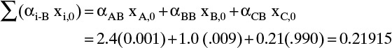
Then the individual mole fractions are calculated from Eq. (8-25b):
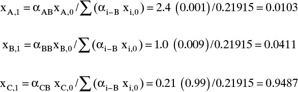
Note that Σxi,1 = 1.0. Increasing j by 1, we can calculate the denominator for j + 1 = 2:
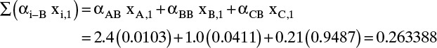
And the individual mole fractions for stage 2 are

Continuing the calculation we generate the following values for the remaining stages:
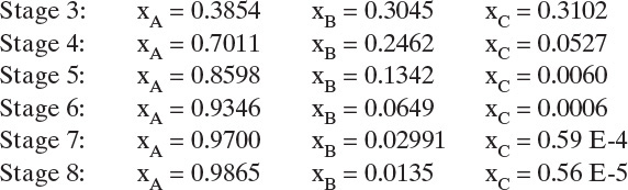
These values were generated from a simple spreadsheet and are plotted in Figure 8-7. Obviously, the calculation can be continued for as many stages as desired. Problem 8.H1 asks that you generate additional values for Figure 8-7.
Solution Part B. Although process simulators determine residue curves, it is again instructive to do a calculation ourselves. This calculation uses Eq. (8-30), starting with still pot mole fractions xA,1 = 0.9905, xB,1 = 0.0085, and xC,1 = 0.001 (where index 1 represents k = 1, which is step 1 in the integration). We first show one hand calculation with h = 0.01.
Hand Calculation: For k = 1,

And Eq. (8-30) is
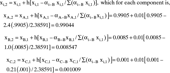
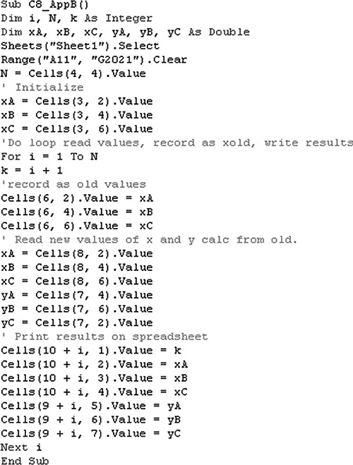
Setting k = 2 in Eq. (8-30), we could continue. This process is obviously laborious to do by hand but can be done in a spreadsheet using VBA to increment the step number, k. This spreadsheet, which does the calculation for h = 0.01 and N (maximum number of iterations) = 1000.0, is shown in Appendix B of this chapter. The results obtained are:
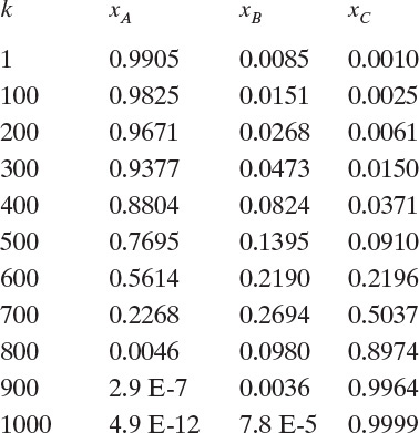
These values can be plotted to form a residue curve that will look similar to Figure 8-7, except the curves should be drawn as smooth curves. Problem 8.H2 provides additional practice generating residue curves. Note: If too large a value of h is used, the recursion formula can give negative mole fractions or mole fractions greater than one. Obviously, these values should not be used.
This completes the introduction to residue curves. Residue curves are used in the explanation of extractive distillation (Section 8.6) and azeotropic distillation (Section 8.7). In Section 9.7 residue curves provide values of y and x needed to solve multicomponent simple batch distillation problems. In Section 11.6 we use residue curves to help synthesize distillation sequences for complex systems. Doherty and Malone (2001) develop properties and applications of residue curves in much more detail than can be done in this introduction.
8.6 Extractive Distillation
Extractive distillation is used for separation of azeotropes and close-boiling mixtures. In extractive distillation, a solvent is added to the distillation column. This solvent is selected so that one of the components being separated, B, is selectively attracted to it. Since solvent is usually chosen to have a significantly higher boiling point than the components being separated, the attracted component B has its volatility reduced. Thus, the other component, A, becomes relatively more volatile and is distillate product. A separate column is required to separate solvent and component B. Residue curves for extractive distillation, after solvent is added, are shown in Figures 8-7 (separation of close-boiling components) and 8-11C (separation of azeotropes).
A typical extractive distillation flowsheet is shown in Figure 8-13. If an azeotrope is being separated, the feed should be close to the azeotrope concentration; thus, a binary distillation column (not shown) usually precedes the extractive distillation system. In column 1 solvent is added several stages above the feed stage and a few stages below the condenser. In the top section, the relatively nonvolatile solvent is removed, and pure A is produced as distillate product. In the middle section, large quantities of solvent are present, and components A and B are separated from each other. It is common to use 1, 5, 10, 20, or even 30 times as much solvent as feed; thus, solvent concentration in the middle section is often quite high. Note that A-B separation must be complete in the middle section because any B that gets into the top section will not be separated (there is very little solvent present) and will contaminate the distillate product. The bottom section strips A from the mixture so that only solvent and B exit in the bottoms product.

The residue curve diagram for extractive distillation of ethanol and water using ethylene glycol as solvent is shown in Figure 8-14. The curves start at the binary azeotrope (89.0% ethanol and 11.0% water), which makes this residue curve plot similar to Figure 8-11C. Since all of the residue curves have the same general shape, there is no distillation boundary in this system. (Compare the shape of the residue curves in Figure 8-14 to those in Figure 8-8, which has a distillation boundary.) The feed to column 1 is 100.0 kmol/h of a mixture that is 72.0 mol% ethanol and 28.0 mol% water. Essentially pure solvent is added at a rate of 52.0 kmol/h. (see Lab 9 in the Chapter 8 appendix). Solvent and feed can be combined as a mixed feed, M, that is found from mass balances.
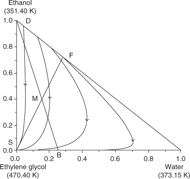
FIGURE 8-14. Residue curves for water-ethanol-ethylene glycol for extractive distillation to break ethanol-water azeotrope. Ravagnani, M. A. S. S., M. H. M. Reis, R. Maciel Filho, M. R. Wolf-Maciel, “Anhydrous Ethanol Production by Extractive Distillation: A Solvent Case Study,” Process Safety and Environmental Protection, 88, 67 (2010). Copyright 2009 The Institution of Chemical Engineers. Published by Elsevier Science
Mixed feed M is then separated in column 1 into streams D and B as shown in Figure 8-14.
Substitution of Eqs. (8-32) in Eqs. (8-31) gives the external mass balances for column 1. Detailed simulations are needed to determine if the solvent flow rate and the reflux ratio are large enough. Increasing the solvent flow rate will move point M toward the solvent vertex.
Residue curves from D to B both stop at S. Extractive distillation works because the solvent is added to the column several stages above the feed stage. Complete analysis of extractive distillation is beyond this introductory treatment. Doherty and Malone (2001) provide detailed information on use of residue curve maps to design extractive distillation systems. Although this extractive distillation can be used to break the ethanol-water azeotrope, azeotropic distillation (see Section 8.7) is more economical.
The mixture of solvent and B is sent to column 2 where they are separated along line SBW. If the solvent is selected correctly, column 2 can be quite short, since component B is significantly more volatile than the solvent. Recovered solvent can be cooled and recycled to the extractive distillation column. Note that the solvent must be cooled before entering column 1, since its boiling point is significantly higher than the operating temperature of column 1.
Column 2 is a simple distillation that can be designed by the methods discussed in Chapter 4. Column 1 is considerably more complex, but the bubble-point matrix method discussed in Chapter 6 can often be adapted. Since the system is nonideal and K values depend on the solvent concentration, a concentration loop is required in the flowchart shown in Figure 6-1 (Aspen Plus automatically includes this loop). Fortunately, a good first guess of solvent concentrations can be made. Solvent concentration will be almost constant in the middle and bottom sections except for the reboiler. In the top section, solvent concentration will very rapidly decrease to zero. Solvent concentrations will be relatively unaffected by temperatures and flow rates. K values can be calculated from Eq. (2-35) with activity coefficients determined from the appropriate VLE correlation. Process simulators are the easiest way to do these calculations (see the Chapter 8 appendix).
Concentration profiles for extractive distillation of n-heptane and toluene using phenol as solvent are shown in Figure 8-15 (Seader, 1984). Profiles were rigorously calculated using a simultaneous correction method, and activity coefficients were calculated with the Wilson equation. Feed was a mixture of 200.0 lbmol/h of n-heptane and 200.0 lbmol/h of toluene input as a liquid at 200.0°F on stage 13. The recycled solvent is input on stage 6 at a total rate of 1200.0 lbmol/h. There are a total of 21 equilibrium contacts including the partial reboiler. High-boiling phenol is attractive to the toluene, since both are aromatics. Heptane is then relatively more volatile and exits in the distillate (component A in Figure 8-13). Note from Figure 8-15 that phenol concentration very rapidly decreases above stage 6, and n-heptane concentration increases. From stages 6 to 12, phenol concentration is approximately constant, and toluene is separated from heptane. From stages 13 to 20, phenol concentration is again constant but at a lower concentration. This change in the solvent (phenol) concentration occurs because the feed is input as a liquid. A constant solvent concentration can be obtained by vaporizing the feed or by adding some recycled solvent to it. Heptane is stripped from the mixture in stages 13 to 20. In the reboiler, the solvent is nonvolatile compared to toluene. Thus, boilup is much more concentrated in toluene than in phenol, which causes the large increase in phenol concentration seen for stage 21 in Figure 8-15. Concentration profiles for other extractive distillation systems are shown by Robinson and Gilliland (1950), Siirola and Barnicki (1997), Doherty and Malone (2001), and Doherty et al. (2008).
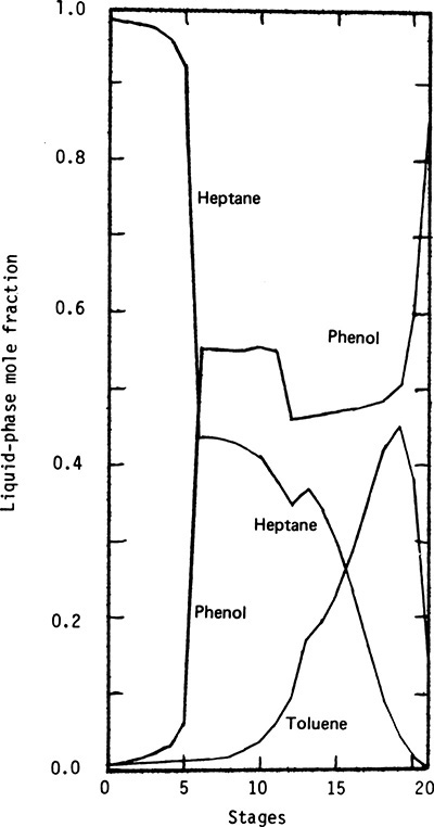
FIGURE 8-15. Calculated composition profiles for extractive distillation of toluene and n-heptane; from Seader (1984), reprinted with permission from Perry’s Chemical Engineer’s Handbook, 6th ed., copyright 1984, McGraw-Hill
The almost constant phenol (solvent) concentrations above and below the feed stage in Figure 8-15 allow for development of approximate calculation methods (Knickle, 1981). A pseudo-binary McCabe-Thiele diagram can be used for separation of heptane and toluene. The equilibrium curve represents y-x data for heptane and toluene with constant phenol concentration. The equilibrium curve will have a discontinuity at the feed stage. For stages above the solvent feed stage, a standard, heptane-phenol binary McCabe-Thiele diagram can be used. Knickle also discusses modifying the Fenske-Underwood-Gilliland (FUG) approach by modifying the relative volatility to represent heptane-toluene equilibrium at the phenol concentration on the feed stage.
The reason for the large increase in solvent concentration in the reboiler can be explained if we look at an extreme case in which none of the solvent vaporizes in the reboiler. Then the boilup is essentially pure component B. The liquid flow rate in the column can be split up as
where S is the constant solvent flow rate; Bliq is the flow rate of component B, which stays in the liquid in the reboiler; and ![]() is the flow rate of the vapor, which is mainly B. The bottoms flow rate consists of the streams that remain liquid:
is the flow rate of the vapor, which is mainly B. The bottoms flow rate consists of the streams that remain liquid:
The mole fraction of component B in the liquid in the column can be estimated as
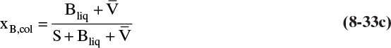
and the mole fraction B in the bottoms is
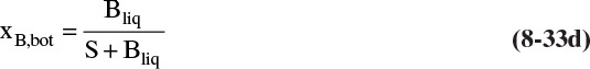
For the usual flow rates this gives xB,col >> xB,bot. Even when solvent is fairly volatile, as in Figure 8-15, toluene (component B) concentration drops in the reboiler.
The behavior of distillation systems in which an entrainer is added to break an azeotrope and recover the two components as pure products (e.g., the homogeneous systems illustrated in Figure 8-11, which include extractive distillation) is often different from the behavior of more ideal ternary distillation systems (Doherty and Malone, 2001; Laroche et al., 1992). For example, feasible operation may require recovering the middle component as distillate from the first column, not the light component as is normally expected. We normally expect that adding trays reduces the reflux ratio needed, but with homogeneous azeotropic systems including extractive distillation, adding trays may increase the required reflux ratio. Similarly, increasing the reflux ratio past an optimum value may cause product purities to decrease, and poor separation is observed at total reflux.
Solvent selection is extremely important. The process is similar to that of selecting a solvent for liquid-liquid extraction (see Chapter 13). By definition, solvent should not form an azeotrope with any of the components (Figure 8-11C). If solvent does form an azeotrope, the process is classified as azeotropic distillation (see Section 8.7). Usually, a solvent is selected that is more similar to the heavy key (HK) to reduce volatility of the HK. Exceptions to this rule exist; for example, for n-butane–1-butene separation, furfural decreases volatility of 1-butene, which is more volatile (Shinskey, 1984). Lists of solvents (Doherty et al., 2008; Van Winkle, 1967) for extractive distillation are helpful in finding a general structure that effectively increases volatility of the keys. Salts including ionic liquids can be used as solvent, particularly when there are small amounts of water to remove (Fu, 1996; Furter, 1993; Mahdi et al., 2015). Residue curve analysis is also very helpful to ensure that solvent does not form additional azeotropes (Biegler et al., 1997; Doherty and Malone, 2001; Julka et al., 2009).
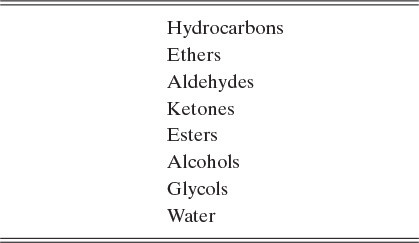
Solvent selection can be aided by considering the polarities of the compounds to be separated. Table 8-1 lists classes of compounds arranged in order of increasing polarity. If two compounds of different polarity are to be separated, a solvent can be selected to attract either the less or the more polar compound. For example, acetone (a ketone boiling at 56.5°C) and methanol (an alcohol boiling at 64.7°C) form an azeotrope. We could add a hydrocarbon to attract acetone. If enough hydrocarbon were added, methanol would become more volatile. A simpler alternative is to add water, which attracts methanol and makes acetone more volatile. Methanol and water are then separated in column 2. In this example, another alternative is to add a higher molecular weight alcohol such as butanol to attract methanol.
Hydrocarbons with double bonds are attracted to polar solvents. For example, furfural decreases volatility of butenes compared to butanes. Furfural (a cyclic alcohol) is used instead of water because it is miscible with hydrocarbons. A more detailed analysis of solvent selection shows that hydrogen bonding is more important than polarity (Berg, 1969; Doherty et al., 2008; Smith, 1963).
Once a general structure has been found, homologs of increasing molecular weight can be checked to find which has a high enough boiling point to be easily recovered in column 2. However, too high a boiling point is undesirable because the solvent recovery column would have to operate at too high a temperature. Solvent should be completely miscible with both components over the entire composition range of the distillation.
It is desirable to use a solvent that is nontoxic, nonflammable, noncorrosive, and nonreactive. In addition, it should be readily available and inexpensive since solvent makeup and inventory costs can be relatively high. Environmental effects and life-cycle costs of various solvents need to be included in the decision (Allen and Shonnard, 2002). Water satisfies these requirements and is often used as a solvent for separation of oxygenated compounds such as acetone + methanol (Mahdi et al., 2015). As usual, designers must make tradeoffs in selecting a solvent. One common compromise is to use a solvent that is used elsewhere in the plant or is a by-product of a reaction even if it may not be the optimum solvent otherwise.
For isomer separations, extractive distillation usually fails, since solvent has the same effect on both isomers. For example, Berg (1969) reports that the best entrainer for separating m- and p-xylene increased the relative volatility from 1.02 to 1.029. An alternative to normal extractive distillation is to use a solvent that preferentially and reversibly reacts with one of the isomers (Doherty and Malone, 2001). The process scheme is similar to Figure 8-14, with the light isomer being product A and the heavy isomer product B. The forward reaction occurs in the first column, and the reaction product is fed to the second column. The reverse reaction occurs in column 2, and the reactive solvent is recycled to column 1. This procedure is quite similar to the combined reaction distillation discussed in Section 8.8.
8.7 Azeotropic Distillation with Added Solvent
When a homogeneous azeotrope is formed or a mixture is very close boiling, the procedures shown in Section 8.2 cannot be used. However, a solvent (or entrainer) that forms a binary or ternary azeotrope can be added that will enable separation. The trick is to pick a solvent that forms an azeotrope that is either heterogeneous (then procedures of Section 8.2 are useful) or easy to separate by other means such as extraction with a water wash. Since there are now three components, it is possible to have one or more binary azeotropes or a ternary azeotrope. The flowsheet depends up the system’s equilibrium behavior, which can be investigated with distillation curves and residue curves (Section 8.5). Most applications of azeotropic distillation use a volatile solvent and are applied to systems with minimum-boiling azeotropes (Mahdi et al., 2015). A few typical examples are illustrated here.
Figure 8-16 shows a simplified flowsheet (extensive heat exchange is not shown) for separation of butadiene from butylenes using liquid ammonia as an entrainer (Poffenberger et al., 1946). The intermediate reboiler in the azeotropic distillation column minimizes polymerization. At 40.0°C the azeotrope is homogeneous. Ammonia can be recovered by cooling, since at temperatures below 20.0°C, two liquid phases are formed. As the settler temperature is reduced the two liquid phases become purer. At –40.0°C, used in commercial plants during World War II, the liquid ammonia phase contained about 7.0 wt% butylene. This stream is recycled to the azeotropic column either as reflux or on stage 30. The top phase fed to the stripping column contains about 5.0 wt% ammonia. The azeotrope formed in the stripping column is recycled to the separator. This example illustrates the following general points: (1) Azeotropes formed are often cooled to obtain two phases and/or to optimize operation of liquid-liquid settlers, (2) streams obtained from settlers are seldom pure and have to be further purified, and (3) product (butylene) can often be recovered from solvent (NH3) in a stripping column instead of a complete distillation column because the azeotrope is recycled.
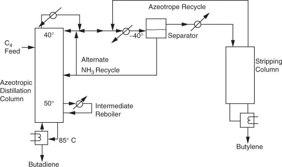
FIGURE 8-16. Separation of butadiene from butylenes using ammonia as an entrainer (Poffenberger et al., 1946)
Another system with a single binary azeotrope is shown in Figure 8-17 (Smith, 1963). In the azeotropic column, component A and the entrainer form a minimum-boiling azeotrope, which is recovered as distillate. The other component, B, is recovered as a pure bottoms product. In this case the azeotrope formed is homogeneous, and a water wash (extraction using water) is used to recover solvent from the desired component with which it forms an azeotrope. Product from the water wash column is almost pure A. A simple distillation column is required to recover solvent from water. Since water always has some solubility in organics, there will be a small amount of water in the A product. Makeup water is added to compensate for this outflow. Chemical systems using flow diagrams similar to this include separation of cyclohexane (A) and benzene (B), using acetone as solvent, and removal of impurities from benzene with methanol as solvent.
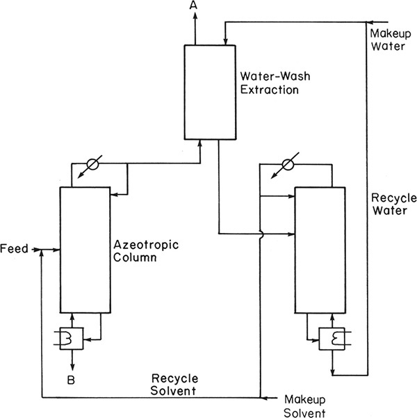
FIGURE 8-17. Azeotropic distillation with one minimum-boiling binary azeotrope; use of water wash for solvent recovery from Smith (1963)
A third example that is quite common is the separation of the ethanol-water azeotrope using a hydrocarbon as solvent, which is called an entrainer in azeotropic distillation. Benzene used to be the most common entrainer (the residue curve is shown in Figure 8-12), but because of its toxicity, it has been replaced by diethyl ether, n-pentane, or n-hexane. A heterogeneous ternary azeotrope is removed as distillate product from the azeotropic distillation column. A typical flowsheet for this system is shown in Figure 8-18 (Black, 1980; Doherty and Malone, 2001; Doherty et al., 2008; Robinson and Gilliland, 1950; Seader, 1984; Shinskey, 1984; Smith, 1963; Widagdo and Seider, 1996). Feed to the azeotropic distillation column is the distillate product from a binary ethanol-water column and is close to azeotropic composition. Composition of the ternary azeotrope varies slightly depending on the entrainer chosen. For example, when n-hexane is the entrainer, the azeotrope contains 85.0 wt% hexane, 12.0 wt% ethanol, and 3.0 wt% water (Shinskey, 1984). The water-ethanol ratio in the ternary azeotrope must be greater than the water-ethanol ratio in the feed so that all water can be removed with the azeotrope and excess ethanol becomes pure bottoms product. The upper layer in the separator is 96.6 wt% hexane, 2.9 wt% ethanol, and 0.5 wt% water, while the bottom layer is 6.2 wt% hexane, 73.7 wt% ethanol, and 20.1 wt% water. The upper layer is refluxed to the azeotropic distillation column, while the bottom layer is sent to a stripping column to remove water. Since very small amounts of hydrocarbon entrainer exit in the product streams, a small makeup solvent addition is required.
Calculations for azeotropic distillation systems are considerably more complex than for simple distillation or even for extractive distillation. This complexity arises from very nonideal equilibrium behavior and from possible formation of three phases (two liquids and a vapor) inside the column. The residue curve shown in Figure 8-12 clearly demonstrates the complexity of these systems. Calculation procedures for azeotropic distillation are reviewed by Doherty and Malone (2001), Prokopakis and Seider (1983), and Widago and Seider (1996).
Simulation results are presented by many authors, including Black (1980), Prokopakis and Seider (1983), Robinson and Gilliland (1950), Seader (1984), Smith (1963), and Widago and Seider (1996). Seader’s results for dehydration of ethanol using n-pentane as solvent are plotted in Figure 8-19. The azeotropic distillation is similar to the flowsheet shown in Figure 8-18. The feed contains 80.94 mol% ethanol, and the pressure is 331.5 kPa to allow condensation of distillate with cooling water. The column has 18 stages, a partial reboiler, and a total condenser. The feed is input on the third stage below the condenser. Note that the profiles are different from those shown in Chapter 5. The pentane appears superficially to be a light key (LK) except that none of it appears in the bottoms. Instead, a small amount of water exits in the bottoms with ethanol.
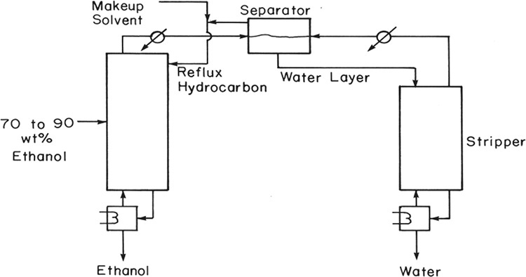
FIGURE 8-18. Ternary azeotropic distillation for separation of ethanol-water with hydrocarbon entrainer
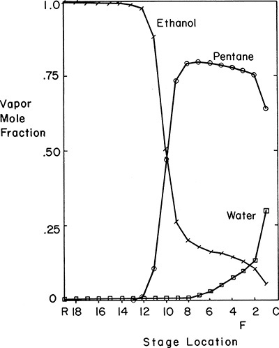
FIGURE 8-19. Composition profiles for azeotropic distillation column separating water and ethanol with n-pentane entrainer (Seader, 1984)
Selecting a solvent for azeotropic distillation is often more difficult than for extractive distillation. Few solvents are available that form azeotropes that boil at a low enough temperature to be easy to remove in distillate or boil at a high enough temperature to be easy to remove in bottoms. Distillation curve and residue curve analyses are useful for screening prospective solvents and for developing new processes (Biegler et al., 1997; Doherty and Malone, 2001; Julka et al., 2009; Widago and Seider, 1996). In addition, binary and ternary azeotropes formed must be easy to separate. In practice, this requirement is met by heterogeneous azeotropes and by azeotropes that are easy to separate with a water wash. The entrainer must also satisfy the usual requirements of being nontoxic, noncorrosive, chemically stable, readily available, inexpensive, and green. Azeotropic distillation systems with unique solvents are patentable.
8.8 Distillation with Chemical Reaction
Although reactions in distillation columns are usually undesirable thermal decomposition, distillation columns are occasionally used as chemical reactors. Advantages of this approach are that distillation and reaction can take place simultaneously in one vessel, and products can be removed to drive a reversible reaction to completion. The most common industrial applications is for the formation of esters from a carboxylic acid and an alcohol. For example, the manufacture of methyl acetate by reactive distillation was a major success with which conventional processes could not compete (Biegler et al., 1997). Reactive distillation was first patented by Backhaus in 1921 and has since been the subject of many patents (see Doherty and Malone, 2001; Doherty et al., 2008; and Siirola and Barnicki, 1997, for references).
Distillation with reaction is useful for reversible reactions. For example, the reversible methyl acetate reaction is
Acetic acid + methanol → methyl acetate + water
The purposes of reactive distillation are to separate product(s) from reactant(s) to drive reactions to right and to recover purified product(s).
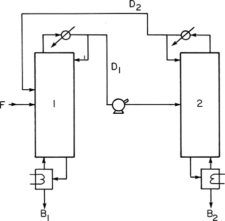
Depending on system equilibrium properties, different distillation configurations can be used (Figure 8-20). Figure 8-20A shows a system in which the reactant is less volatile than the product (Belck, 1955). If several products are formed, no attempt is made to separate them in this system. The bleed is used to prevent buildup of nonvolatile impurities or products of secondary reactions. If the feed is more volatile than the desired product, the arrangement shown in Figure 8-20B can be used (Belck). Columns in Figures 8-20A and 8-20B are essentially at total reflux except for small bleeds, which may be needed to remove impurities, volatiles, or gases.
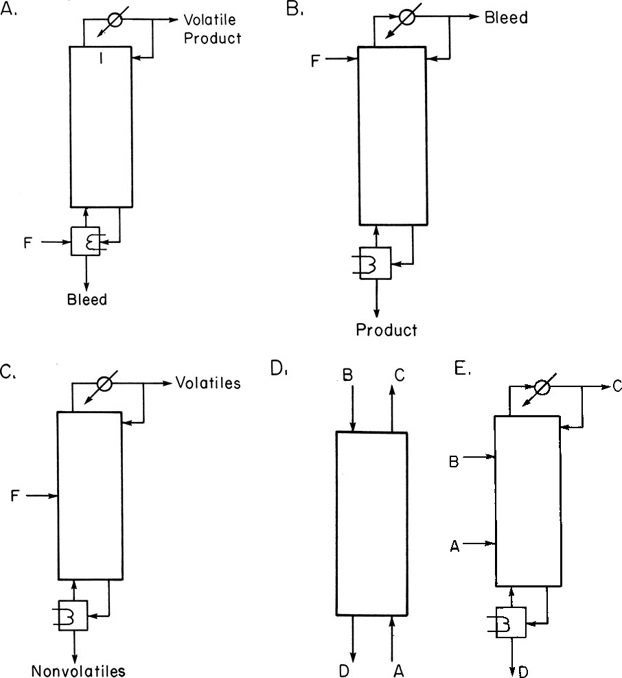
FIGURE 8-20. Schemes for distillation plus reaction: (A) Volatile product, reaction is A = C; (B) nonvolatile product, reaction is A = D; (C) two products, reactions are A = C + D or A + B = C + D; (D, E) reaction A + B = C + D with B and D nonvolatile.
Figures 8-20C, 8-20D, and 8-20E show systems in which two products are formed and separated from each other and from the reactants. In Figure 8-20C, since reactant(s) are of intermediate volatility between the two products, they will stay in the middle of the column until they are consumed. Products are continuously removed, driving the reaction to the right. If the reactants are not of intermediate volatility, some of the reactants will appear in each product stream (Suzuki et al., 1971). Alternative schemes, as shown in Figures 8-20D and 8-20E (Siirola and Barnicki, 1997; Suzuki et al., 1971), are often advantageous for reaction:
A + B = C + D
In Figures 8-20D and 8-20E, species A and C are relatively volatile, while species B and D are relatively nonvolatile. Since reactants are fed in at opposite ends of the column, there is a large region where both reactants are present. Thus, the residence time for the reaction will be larger in Figures 8-20D and E than in Figure 8-20C, and higher yields can be expected. The systems shown in Figures 8-20C and 8-20D have been used for esterification reactions such as
Acetic acid + ethanol → ethyl acetate + water
(Suzuki et al., 1971) and for the production of methyl acetate shown earlier. Siirola and Barnicki (1997) show a four-component residue curve map for methyl acetate production. They used a modification of Figure 8-20E in which a nonvolatile liquid catalyst is fed between acetic acid (B) and methanol (A) feeds.
When a reaction occurs in the column, the mass and energy balance equations must be modified to include the reaction terms. The general mass balance equation for stage j (Eq. 6-1) becomes
where reaction term ri,j is positive if the component is a product of the reaction. To use Eq. (8-34), an appropriate rate equation must be used for ri,j. In general, reaction rate depends on temperature and the liquid compositions.
When mass balances are in matrix form, reaction terms can conveniently be included with the feed in the D term in Eqs. (6-6) and (6-13). This retains the mass balance’s tridiagonal form, but the D term depends on the liquid concentration and the stage temperature, which make the equations highly nonlinear. Modern process simulators are usually able to converge for reactive distillation problems, although it may be necessary to change convergence procedures or properties.
A sample of composition and temperature profiles for esterification of acetic acid and ethanol is shown in Figure 8-21 (Suzuki et al., 1971) for the distillation system of Figure 8-20C. The distillation column is numbered with Aspen Plus notation (total condenser = 1, and partial reboiler = 13). Reaction can occur on every stage and in the condenser and the reboiler. The feed is introduced to stage 6 as a saturated liquid. The feed is mainly acetic acid and ethanol with a small amount of water. A reflux ratio of 10 is used. The top product contains most of the ethyl acetate product plus ethanol and a small amount of water. All unreacted acetic acid appears in bottoms along with most of the water and a significant fraction of the ethanol. Reaction is obviously not complete.
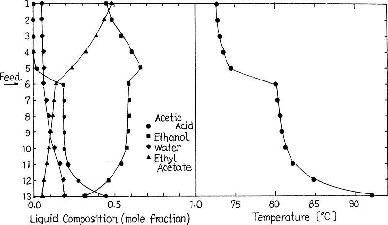
FIGURE 8-21. Composition and temperature profiles for the reaction acetic acid + ethanol = ethyl acetate + water, from Suzuki et al. (1971), copyright 1971. Reprinted with permission from Journal of Chemical Engineering of Japan.
A somewhat different type of distillation with reaction is catalytic distillation (Doherty et al., 2008). In this process bales of catalyst are stacked in the column. The bales serve both as catalyst and as column packing (see Chapter 10). This process was used commercially for the production of methyl tert-butyl ether (MTBE) from liquid-phase reaction of isobutylene and methanol. Heat generated by the exothermic reaction was used to supply much of the heat required for distillation. Since MTBE use as a gasoline additive has been outlawed because of pollution problems from leaky storage tanks, these units are shut down. Other applications of catalytic distillation include desulfurization of gasoline, separation of 2-butene from a mixed C4 stream, esterification of fatty acids, and etherification.
Although many reaction systems do not have the right reaction equilibrium or VLE characteristics for distillation with reaction, for those that do, this technique is a valuable industrial tool.
References
Allen, D. T., and D. R. Shonnard, Green Engineering: Environmentally Conscious Design of Chemical Processes, Prentice Hall, Upper Saddle River, NJ, 2002.
Belck, L. H., “Continuous Reactions in Distillation Equipment,” AIChE J., 1, 467 (1955).
Berg, L., “Selecting the Agent for Distillation Processes,” Chem. Engr. Progr., 65 (9), 52 (Sept. 1969).
Biegler, L. T., I. E. Grossmann, and A. W. Westerberg, Systematic Methods of Chemical Process Design, Prentice Hall, Upper Saddle River, NJ, 1997.
Black, C., “Distillation Modeling of Ethanol Recovery and Dehydration Processes for Ethanol and Gasohol,” Chem. Engr. Progr., 76 (9), 78 (Sept. 1980).
Chambers, J. M., “Extractive Distillation, Design and Application,” Chem. Engr. Progr., 47, 555 (1951).
Chu, J. C., R. J. Getty, L. F. Brennecke, and R. Paul, Distillation Equilibrium Data, Reinhold, New York, 1950.
DDBST, www.ddbst.com/en/EED/AZD/AZDBenzene%3BWater.php, accessed June 6, 2016.
Doherty, M. F., Z. T. Fidkowski, M. F. Malone, and R. Taylor. “Distillation,” in D. W. Green and R. H. Perry (Eds.), Perry’s Chemical Engineer’s Handbook, 8th ed., McGraw-Hill, New York, Section 13 (2008).
Doherty, M., and M. Malone, Conceptual Design of Distillation Systems, McGraw-Hill, New York, 2001.
Drew, J. W., “Solvent Recovery,” in P. A. Schweitzer (Ed.), Handbook of Separation Techniques for Chemical Engineers, 3rd ed., McGraw-Hill, New York, 1997, Section 1.6.
Frank, T. C., “Break Azeotropes with Pressure-Sensitive Distillation,” Chem. Engr. Prog., 93 (4) 52 (April 1997).
Fu, J., “Salt-Containing Model for Simulation of Salt-Containing Extractive Distillation,” AIChE Journal, 42 (12), 3363 (Dec. 1996).
Furter, W. F., “Production of Fuel-Grade Ethanol by Extractive Distillation Employing the Salt Effect,” Separ. Purific. Methods, 22, 1 (1993).
Hengstebeck, R. J., Distillation: Principles and Design, Reinhold, New York, 1961.
Julka, V., M. Chiplunkar, and L. O’Young, “Selecting Entrainers for Azeotropic Distillation,” Chem. Engr. Progress, 105 (3), 47 (March 2009).
Knickle, H. N., “Extractive Distillation,” AIChE Modular Instruction, Series B: Stagewise and Mass Transfer Operations, Vol. 2: Multicomponent Distillation, AIChE, New York, 1981, pp. 50–59.
Kovach, J. W., III, and W. D. Seider, “Heterogeneous Azeotropic Distillation: Experimental and Stimulation Results,” AIChE J., 33 (8), 1300 (Aug. 1987).
Laroche, L., N. Bekiaris, H. W. Anderson, and M. Morari, “The Curious Behavior of Azeotropic Distillations—Implications for Entrainer Selection,” AIChE J., 38 (9), 1309 (Sept. 1992).
Ludwig, E. E., Applied Process Design, 3rd ed., Vol. 2, Gulf Publishing Co., Houston, 1997.
Luyben, W. L., “Azeotropic Tower Design by Graph,” Hydrocarbon Processing, 52 (1), 109 (Jan. 1973).
Mahdi, T., A. Ahmad, M. M. Nasef, and A. Ripin, “State-of-the-Art Technologies for Separation of Azeotropic Mixtures,” Separ Purific. Rev., 44, 308 (2015).
Perry, R. H., and D. W. Green (Eds.), Perry’s Chemical Engineers’ Handbook, 7th ed., McGraw-Hill, New York, 1997.
Poffenberger, N., L. H. Horsley, H. S. Nutting, and E. C. Britton, “Separation of Butadiene by Azeotropic Distillation with Ammonia,” Trans. Amer. Inst. Chem. Eng., 42, 815 (1946).
Prokopakis, G. J., and W. D. Seider, “Dynamic Simulation of Azeotropic Distillation Towers,” AIChE J., 29, 1017 (1983).
Ravagnani, M. A. S. S., M. H. M. Reis, R. Maciel Filho, and M. R. Wolf-Maciel, “Anhydrous Ethanol Production by Extractive Distillation: A Solvent Case Study,” Process Safety and Environmental Protection, 88, 67 (2010).
Robinson, C. S., and E. R. Gilliland, Elements of Fractional Distillation, 4th ed., McGraw-Hill, New York, 1950, Chapter 10.
Seader, J. D., “Distillation,” in R. H. Perry and D. W. Green (Eds.), Perry’s Chemical Engineers’ Handbook, 6th ed., McGraw-Hill, New York, 1984, Section 13.
Shinskey, F. G., Distillation Control for Productivity and Energy Conservation, 2nd ed., McGraw-Hill, New York, 1984, Chapters 9 and 10.
Siirola, J. J., and S. D. Barnicki, “Enhanced Distillation,” in R. H. Perry and D. W. Green (Eds.), Perry’s Chemical Engineers’ Handbook, 7th ed., McGraw-Hill, New York, pp. 13–54 to 13–85, 1997.
Skiborowski, M., A. Harwardt, and W. Marquardt, “Conceptual Design of Azeotropic Distillation Processes,” in A. Gorak and E. Sorenson (Eds.), Distillation: Fundamentals and Principles, Elsevier, London, UK, 2014, Chapter 8.
Smith, B. D., Design of Equilibrium Stage Processes, McGraw-Hill, New York, 1963, Chapter 11.
Speight, J. (Ed.) Lange’s Handbook of Chemistry, 70th Anniversary Edition, 16th ed., McGraw-Hill, New York, 2005.
Suzuki, I., H. Yagi, H. Komatsu, and M. Hirata, “Calculation of Multicomponent Distillation Accompanied by a Chemical Reaction,” J. Chem. Eng. Japan, 4, 26 (1971).
Van Winkle, M., Distillation, McGraw-Hill, New York, 1967.
Wankat, P. C., Separation Process Engineering, 2nd ed., Prentice-Hall, Upper Saddle River, NJ, 2007.
Wasylkiewicz, S. K., “Troubleshooting Distillation Simulation,” Chem. Engr. Prog, 102 (6), 22 (June 2006).
Widago, S., and W. D. Seider, “Azeotropic Distillation,” AIChE Journal, 42, 96 (1996).
Homework
A. Discussion Problems
A1. Why is water often used as a solvent in extractive distillation?
A2. Explain why you can use a constant value of h in Eq. (8-30) when H decreases and V may not be constant.
A3. Why is a cooler required in Figure 8-13? How can this energy be reused in the process?
A4. Explain the purpose of the liquid-liquid settler in Figures 8-3A, 8-4A, and 8-18.
A5. Explain why the external mass balances are the same for Figures 8-3A and 8-6.
A6. Why are makeup solvent additions shown in Figures 8-13, 8-17, and 8-18?
A7. Explain why extra stages are not usually helpful in steam distillation.
A8. When will extra stages be helpful in steam distillation?
A9. When doing distillation with reaction, the column should be designed both as a reactor and as a distillation column. How might these columns differ from normal distillation columns?
A10. Reactions are usually not desirable in distillation columns. If there is a reaction occurring, what can be done to minimize it?
A11. Develop your key relations chart for this chapter.
A12. If a liquid mixture of n-butanol and water that is 20.0 mol% n-butanol is vaporized, what is the vapor composition? (See Figure 8-2.) Repeat for mixtures that are 10.0 mol%, 30.0 mol%, and 40.0 mol% n-butanol. Explain what is happening.
A13. Extractive distillation (Figure 8-13) is used to separate ethanol from water with ethylene glycol as solvent. The A product will be ethanol and the B product water. Stages are counted with condenser = 1 and reboiler = N. The feed plate for the solvent recycle in column 1 is = NS. The feed stages are NF1 in column 1 and NF2 in column 2. Pick the best solution of the listed items.
1. If too much solvent is found in the water product:
a. Increase L/D in column 1.
b. Increase the value of NS.
c. Increase the number of stages in the stripping section of column 1.
d. Increase the number of stages in the stripping section of column 2.
e. Increase the number of stages in the enriching section of column 2.
2. If excessive water is in the ethanol product when fresh solvent is added (no solvent recycle):
a. Increase L/D in column 1.
b. Increase the solvent rate.
c. Increase the value of NS.
d. Increase the number of stages in the stripping section of column 1.
3. If excessive water is in the ethanol product with solvent recycle but was not with the fresh solvent:
a. Increase L/D in column 1.
b. Increase the value of NS.
c. Increase the number of stages in the stripping section of column 1.
d. Reduce the water in the bottoms of column 2.
4. If excessive ethanol is found in the water product:
a. Increase L/D in column 1.
b. Increase the value of NS.
c. Increase the number of stages in the stripping section of column 1.
d. Reduce the water in the bottoms of column 2.
e. Increase the number of stages in the enriching section of column 2.
5. If too much solvent is in the ethanol product:
a. Increase L/D in column 1.
b. Increase the value of NF1.
c. Increase the number of stages in the stripping section of column 1.
d. Reduce the water in the bottoms of column 2.
B. Generation of Alternatives
B1. We wish to separate two organics that form a homogeneous azeotrope. This will be done in a two-column azeotropic system with water as the solvent. Sketch possible system arrangements to do this.
C. Derivations
C1. Derive Eq. (8-7) for the two-column, binary heterogeneous azeotrope system.
C2. An equation for αorg–w in w similar to Eq. (8-13) is easy to derive; do it. Compare the predicted equilibrium in water with the butanol-water equilibrium data given in Problem 8.D2. Comment on the fit. Vapor pressure data are in Perry and Green (1984). Use data in Table 8-2 for solubility data.
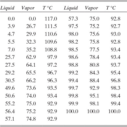
Source: Chu et al. (1950). mol% water. Data at 0% water are from Perry and Green (1984).
TABLE 8-2. VLE data for water and n-butanol at 1.0 atm mol% water
C3. For a binary heterogeneous azeotrope separation, feed can be introduced into the liquid-liquid separator. In this case two stripping columns are used.
a. Sketch the column arrangement.
b. Draw the McCabe-Thiele diagram for this system.
c. Compare this system to the system in Figure 8-3A.
C4. Sketch the McCabe-Thiele diagram for a two-pressure system similar to Figure 8-6.
D. Problems
*Answers to problems with an asterisk are at the back of the book.
D1. Nitromethane and water are separated in a rectifying column system with a total condenser and a liquid-liquid settler similar to Figure 8-3A, except the column is a rectifying column. The saturated vapor feed is 7.5 mol% water. The water product from the settler is 91.4 mol% water. The organic phase refluxed to the column is 31.2 mol% water. Pressure = 1.0 atm, feed rate = 50.0 kmol/h, and CMO is valid. The desired bottoms is 2.5 mol% water.
Find: xdist (water mole fraction), reflux ratio L/D, D, B, and the number of equilibrium stages.
Equilibrium data are in Table 8-3, Problem 8.E1. Be sure to read the note on safety at the end of Problem 8.E1.
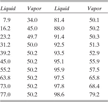
D2. Nitromethane and water are separated in a stripping column that has a partial reboiler. There is no condenser and no liquid-liquid settler. The saturated liquid feed is 8.0 mol% nitromethane and has a feed rate of 100.0 kmol/h. Distillate is a saturated vapor. Bottoms is 1.0 mol% nitromethane. Pressure p = 1.0 atm, and CMO is valid. ![]() .
.
Find ydist (mole fraction nitromethane), B, D, and the number of equilibrium stages. Equilibrium data are in Table 8-3, Problem 8.E1. Be sure to read the note on safety at the end of Problem 8.E1.
D3. VLE data for water and n-butanol are given in Table 8-2. We have flash distillation systems separating 100.0 kmol/h of two different water and n-butanol mixtures.
a. The feed is 20.0 mol% water, and the vapor product is 40.0 mol% water. Find L, x, V, and Tdrum.
b. The feed is 99.0 mol% water, and 30.0% of the feed is vaporized. Find L, x, V, y, and Tdrum.
D4.* VLE data for water–n-butanol are given in Table 8-2. Distill 5000.0 kmol/h of a mixture that is 28.0 mol% water and 30.0% vapor in a two-column azeotropic distillation system. A butanol product that contains 4.0 mol% water and a water product that is 99.5 mol% water are desired. Pressure is 101.3 kPa. Reflux is a saturated liquid. Use L/V = 1.23(L/V)min in the column producing the butanol product. Both columns have partial reboilers. ![]() in the column producing the water product.
in the column producing the water product.
a. Find the flow rates of the products.
b. Find the optimum feed location and the number of stages in the columns.
Note: Draw two McCabe-Thiele diagrams.
D5. 200.0 kmol/h of saturated vapor feed, 80.0 mol% water and 20.0 mol% butanol, is condensed and sent to a decanter. The water layer is the distillate product D, and the butanol (top) layer is sent to a stripping column that has a partial reboiler. The bottoms from the stripping column (B, the butanol product) is 4.0 mol% water. Vapor leaving the stripping column is condensed and sent to the decanter. Equilibrium data are in Table 8-2. Find:
a. Flow rates D and B.
b. If ![]() , find the number of equilibrium stages (step off from the bottom up).
, find the number of equilibrium stages (step off from the bottom up).
c. Determine ![]() for this separation.
for this separation.
D6. A water–n-butanol mixture is separated in a stripping column with a partial reboiler. The feed (F = 100 kmol/h, z = 0.65 [mole fraction water], saturated vapor) is mixed with vapor leaving the top of the column, and the combined stream is sent to a total condenser and then to a liquid-liquid separator. The top layer from the liquid-liquid settler (xα = xdist = 57.3 mol% water) is sent as a saturated liquid reflux to the distillation column. The bottom layer (xβ = xdist = 97.5 mol% water) is the distillate product. CMO is valid, p = 1.0 atm, reflux is a saturated liquid, boilup ratio ![]() , xbot = 2.0 mol% water.
, xbot = 2.0 mol% water.
a. Find D and B in kmol/h.
b. What is the reflux flow rate, kmol/h?
c. How many stages are required? Step off stages from the top down.
d. What is the minimum value of the boilup ratio?
D7. Aniline and water are partially miscible and form a heterogeneous azeotrope. At p = 778.0 mm Hg the azeotrope concentrations are: vapor is 3.64 mol% aniline, liquid aqueous phase contains 1.48 mol% aniline, and the liquid organic phase contains 62.8 mol% aniline. Estimate the relative volatility of water with respect to aniline in the organic phase. Note: Be careful to use mole fractions of the correct component.
D8.* 15,000 kg/h of saturated liquid diisopropyl ether (C6 H14 0) that contains 0.4 wt% water is fed to the system in Figure 8-4, operating at 101.3 kPa. Diisopropyl ether product should contain 0.04 wt% water. Assume CMO is valid. L/D = 1.5(L/D)min. Data for heterogeneous diisopropyl ether–water azeotrope: y = 0.959; separator: top layer x = 0.994, bottom layer x = 0.012; 101.3 kPa; and 62.2°C. (Trans. AIChE, 36, 593, 1940). All compositions are weight fractions of diisopropyl ether. Estimate αw–ether in ether from these data (in mole fraction units). Assume this relative volatility is constant. Determine (L/D)min, L/D, the optimum feed stage, and the total number of stages required.
a. 200.0 kmol/h of a saturated liquid feed is fed to a kettle partial reboiler at 1.0 atm. The feed is water saturated with n-butanol. The vapor at a flow rate V = D is withdrawn with n-butanol distillate mole fraction ydist = 0.15. Find xbot (n-butanol mole fraction), B, and D.
b. 150.0 kmol/h of a saturated liquid feed is fed to a kettle partial reboiler at 1.0 atm. The feed is n-butanol saturated with water (point β in Figure 8-4 B). Bottoms is withdrawn at flow rate L = B at water bottoms mole fraction xbot = 0.40. Find ydist (water mole fraction), B, and D.
Equilibrium data for Parts a and b are in Table 8-2 in Problem 8.D3.
D10.* A single-stage steam distillation system is recovering n-decane from a small amount of nonvolatile organics. Pressure is 760.0 mm Hg. The still is operated with liquid water present, and the organic layer in the still is 99.0 mol% n-decane. Determine:
a. Still temperature.
b. Moles of water vaporized per mole of n-decane vaporized.
Decane vapor pressure is in Example 8-2. Water vapor pressures are (T in °C and VP in mm Hg) (Perry and Green, 1997).
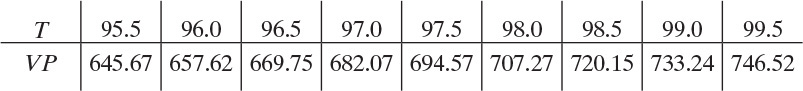
D11. A single-stage, continuous steam distillation of 1-octanol at 760.0 mm Hg with liquid water present distils 1.0 kmol/h of a feed of 90.0 mol% 1-octanol and the rest nonvolatile compounds. Distillate vapor is condensed, and two immiscible liquid layers form. Flow rate of the feed is 1.0 kmol/h. We desire to recover 95.0% of 1-octanol. Water vapor pressure data can be fit to Antoine equation as
log10(VPwater) = 8.68105 – 2164.42/(T + 273.16)
Vapor pressure of 1-octanol is predicted by the Antoine equation (Speight, 2005):
Log10(VPoctanol) = 6.8379 – 1310.2/(T + 136.05)
In both, Antoine equation VP is vapor pressure in mm Hg, and T is in Celsius.
a. Find the operating temperature of the still.
b. Find the octanol mole fraction in the vapor leaving the still.
c. Find the moles of octanol recovered and the moles of water condensed in the distillate product.
D12. Compounds P and Q are separated in a two-pressure distillation system (Figure 8-6). F = 100, zP = 0.4, and zQ = 0.6, and it is a saturated liquid. At the pressure of column 1, p1, component P is more volatile from xP = 0 to xP = xP,Az at P1 = 0.65. Thus, bottoms B1 is Q product. Assuming B1 is pure Q and B2 is pure P, calculate the flow rates of B1 and B2. Then assume the distillate product from column 1, xP,dist,1 = xP,Az at P1, and the distillate product from column 2, xP,dist,2 = xP,Az at P2, and calculate D1 and D2 for following values of the azeotrope in column 2, xP,Az at P2:
a. xP,Az at P2 = 0.55
b. xP,Az at P2 = 0.64
D13. Water is separated from n-butanol in a system with two feeds. Feed 1 (F1 = 100.0 kmol/h, z1 = 0.84 [mole fraction water], saturated vapor) is mixed with vapor leaving the top of the column before it is sent to the total condenser and then to the liquid-liquid settler. Feed 2 (F2 = 80.0 kmol/h, z2 = 0.20 [mole fraction water], saturated liquid) is fed within the column. The column has a partial reboiler, and CMO is valid. The top layer from the liquid-liquid settler (x0 = 57.3 mol% water) is sent as reflux to the distillation column. The bottom layer (xdist = 97.5 mol% water) is the water product. Pressure p = 1.0 atm, reflux is a saturated liquid, ![]() , xbot = 4.0 mol% water. Equilibrium data are in Table 8-2.
, xbot = 4.0 mol% water. Equilibrium data are in Table 8-2.
a. Find D and B in kmol/h.
b. Find ![]() ,
, ![]() in the bottom section of the column, and find V and L in the section above feed 2, both in kmol/h.
in the bottom section of the column, and find V and L in the section above feed 2, both in kmol/h.
c. Derive the operating equation for the distillation section above feed 2 (flow rates V and L).
d. Plot the operating lines, and step off stages starting at the reboiler and going up the column. Use the optimum feed stage for feed 2. Report the optimum feed stage above the partial reboiler and the total number of stages.
D14. A two-pressure system (similar to Figure 8-6) separates a feed that is 15.0 mol% benzene and 85.0 mol% ethanol. The saturated liquid feed rate is 100.0 kmol/h. The columns are at 101.3 kPa and 1333 kPa. The ethanol product is 99.2 mol% ethanol, and the benzene product is 99.4 mol% benzene. Assume the two distillate products are at the azeotrope concentrations.
a. Draw a flowsheet for this process. Label the streams to correspond with your calculations.
b. Find the flow rates of the ethanol and benzene products.
c. Find the flow rates of the two distillate streams that are fed to the other column.
Data (Seader, 1984): Azeotrope is homogeneous. At 101.3 kPa the azeotrope is at 67.9°C and is 44.9 mol% ethanol. At 1333 kPa the azeotrope is at 159°C and is 75.0 mol% ethanol. Ethanol is more volatile at mole fractions below the azeotrope mole fraction.
D15. Continuous steam distillation is used to recover 1-octanol from 100.0 kg/h of feed that is 15.0 wt% 1-octanol, and the remainder consists of nonvolatile organics and solids of unknown composition. The feed is preheated to same temperature as the still pot, which operates at 1.0 atm pressure. Operation is with liquid water in the pot. Assume the still pot is well mixed and the liquid and vapor are in equilibrium. Recover 95.0% of 1-octanol in distillate. Assume water is completely immiscible with 1-octanol and with nonvolatile organics. Because the composition of the nonvolatile organics is not known, we boiled the feed mixture under a vacuum with no water present. The result at 0.05 atm pressure was the mixture boiled at 129.8°C.
a. Find the mole fraction of 1-octanol in the feed and the effective average molecular weight of the nonvolatile organics and solids.
b. Find the kg/h and kmol/h of 1-octanol in distillate, the kg/h of total organics in waste, and the 1-octanol weight fraction and the 1-octanol mole fraction in the waste.
c. Find the temperature of the still pot. A spreadsheet or MATLAB is highly recommended.
d. Find the kg/h and kmol/h of water in distillate.
Octanol boils at about 195°C. The formula for octanol is CH3(CH2)6CH2OH, and its molecular weight is 130.23. Vapor pressure fits for octanol and water are available in Problem 8.D11.
Note: We will see in Problem 9.E2 that batch steam distillation requires less steam than continuous steam distillation.
D16. An extractive distillation system (Figure 8-13) is separating ethanol from water using ethylene glycol as the solvent. The makeup solvent stream is pure ethylene glycol. The feed flow rate is 100.0 kmol/h. The feed is 81.0 mol% ethanol and 19.0 mol% water. The ethanol product (column 1 distillate) is 99.70 mol% ethanol, 0.02 mol% ethylene glycol, and the remainder is water. The water product (column 2 distillate) should be 99.90 mol% water, 0.035 mol% ethylene glycol, and the remainder ethanol. Find the flow rates of the makeup solvent and the distillate from columns 1 and 2.
D17. An extractive distillation system is separating compound A from C with solvent. The solvent flow rate is S, the feed flow rate is F, the entering solvent is pure, and the entering feed is a saturated liquid with mole fractions zA and zC. Because of plant operating problems, the distillate flow rate has to be shut down (D = 0). The values of F, S, Qc, and QR are not changed. After a new steady state is reached, predict the values of B and the mole fractions in the bottoms stream.
D18. An extractive distillation system is separating ethanol from water using ethylene glycol as solvent. The makeup solvent is pure ethylene glycol. In Figure 8-13 ethanol is A product, and water is B product. The feed is 20.00 mol% ethanol, and the remainder is water with flow rate of 100.0 kmol/h. The ethanol product (column 1 distillate) is 99.70 mol% ethanol, 0.02 mol% ethylene glycol, and the remainder is water. The water product (column 2 distillate) is 99.90 mol% water, 0.035 mol% ethylene glycol, and the remainder is ethanol.
a. Find the flow rates of the makeup solvent and of the ethanol and water products.
b. Why would the system in Problem 8.D16 be chosen instead of this system?
D19. The azeotropic distillation shown in Figure 8-18 uses n-hexane as an entrainer to separate a feed that is 80.0 wt% ethanol and 20 wt% water into ethanol and water. The saturated liquid feed is 10,000 kg/h. The ethanol product is 99.999 wt% ethanol, 0.001 wt% hexane, and a trace of water. Water product is 99.998 wt% water, 0.002 wt% ethanol, and a trace of hexane. Do external mass balances, and calculate the flow rates of the make-up solvent (n-hexane), the ethanol product, and the water product. (Assume trace = 0.)
Note: Watch your decimal points when using weight fractions and wt%.
D20. This problem explores the azeotropic distillation column shown in Figure 8-18 with mole fraction profiles shown in Figure 8-19. The feed to the distillation column in Figure 8-18 is a saturated liquid that is 80.94 mol% ethanol with the remainder being water. Do calculations on a basis of 1000.0 kmol/h. The ethanol product is 99.8 mol% ethanol and 0.2 mol% water. The water product is 99.99 mol% water and 0.01 mol% ethanol. In practice there will be traces of pentane in both products, but ignore this (assume makeup solvent = 0). The vapor mole fractions of the compounds leaving the top stage of the distillation column in Figure 8-18 (correspond to the profiles in Figure 8-19) are: ethanol yE,1 = 0.0555, water yw,1 = 0.3000, and pentane yp,1 = 0.6445. Assume water and pentane are totally immiscible; thus, there is no water in the reflux to the distillation column, and there is no pentane in the feed to the stripping column. Ethanol distributes between the water and pentane layers in the settler. In the absence of data assume distribution coefficient
Kd,ethanol = xethanol_in_pentane/xethanol_in_water = 1.0 (x are mole fractions).
CMO is valid in both columns, and operation of the stripping column is at 1.0 atm.
a. Calculate the flow rates of ethanol product E and water product W.
b. What is V1 in the distillation column, and what is the boilup rate in this column? (Note that Vyw,1 must equal water in the feed minus the small amount of water lost in the ethanol product.) Also calculate L0 = reflux rate.
c. Since no pentane enters the stripper, at steady state all pentane that enters the settler must be returned to the distillation column in the reflux stream. In addition, all ethanol entering the settler minus the small amount of ethanol that leaves with the water product must be returned to the distillation column in the reflux stream. Calculate the steady-state values of xethanol_in_pentane and xethanol_in_water and the mole fractions of the reflux stream. Note that xethanol_in_pentane and xethanol_in_water are not equal to yE,1.
d. If the boilup ratio in the stripper is 0.5, what is the flow rate of the liquid fed to the stripper, and what is the flow rate of the vapor leaving the stripper? What is the mole fraction of ethanol in the vapor leaving the top stage of the stripper (yE,1,stripper)?
D21. Water containing 1.6 mol% n-butanol is sent at a rate of 75.0 kmol/h to a two-column distillation system similar to Figure 8-4A. The feed is a saturated liquid. Pressure is 1.0 atm. The column with the feed has a partial reboiler and a total condenser connected to a liquid-liquid separator. The denser aqueous phase (point α) containing 2.5 mol% n-butanol is returned as reflux to the column that receives the feed. Bottoms from this column (the water product) contains 0.2 mol% n-butanol. The organic phase from the settler containing 57.3 mol% water is sent to a stripper that has a partial reboiler. Bottoms from this stripper is n-butanol product and is 4.0 mol% water. The vapor distillate from this column has ydist,water = 0.68 and is condensed and then sent to liquid-liquid separator.
a. Sketch the flowsheet.
b. Find the flow rates of the two products.
c. Find: ![]() ,
, ![]() ,
, ![]() ,
, ![]() , L, V, the optimum feed stage, and the total number of stages needed for the column with the feed (produces water product).
, L, V, the optimum feed stage, and the total number of stages needed for the column with the feed (produces water product).
d. For the stripping column, find ![]() ,
, ![]() , and the number of stages needed.
, and the number of stages needed.
e. For liquid-liquid separator show that total flow in = total flow out and that water flow in = water flow out.
Note: Use diagrams with different scales for parts c and d.
D22. We are separating nitromethane and water in a distillation system consisting of two columns, two total condensers, two partial reboilers, and a liquid-liquid separator. Equilibrium data are in Table 8-3 in Problem 8-E1. CMO is valid, and p = 1.0 atm. There are two feeds to the system. Feed 1 has F1 = 100.0 kmol/h and z1 = 0.15 water (0.85 NM) and is a saturated liquid. Feed 2 has F2 = 80.0 kmol/h and z2 = 0.94 water (0.06 NM) and is a saturated liquid.
Desired results: Water (W) product (flow rate PW kmol/h) contains xNM,PW = 1.0 mol% NM (xW,PW = 0.99). This column has ![]() . Nitromethane (NM) product (flow rate PNM kmol/h) contains xW,PNM = 2.5 mol% W (xNM,PNM = 0.975). This column has
. Nitromethane (NM) product (flow rate PNM kmol/h) contains xW,PNM = 2.5 mol% W (xNM,PNM = 0.975). This column has ![]() .
.
a. Find product flow rates PNM and PW in kmol/h.
b. Sketch the process showing schematically where each feed is located.
c. Find the optimum feed locations and the total number of stages for both columns.
Hint: Derive your operating lines.
D23. 100.0 kmol/h of a saturated vapor feed that is 25.0 mol% nitromethane (NM) and 75.0 mol% water is separated in a system with two distillation columns and a liquid-liquid separator. The feed is sent to column W that produces a water product that is 1.0 mol% NM. The boilup ratio in column W is 1/4. Use the optimum feed stage. The vapor distillate from column W is condensed and sent to the decanter. The water phase from the decanter (8.6 mol% NM) is refluxed to column W. The NM phase from the decanter (31.2 mol% water) is sent to stripping column NM. The nitromethane product from the bottom of stripping column NM is 2.0 mol% water. The boilup ratio in column NM = 3.0. Assume both columns operate at 1.0 atm pressure, CMO is valid, both condensers are total condensers, and both reboilers are partial reboilers. Equilibrium data are in Table 8-3 in Problem 8-E1. Find:
a. The flow rates of both products.
b. The optimum feed plate location and the number of stages in column W. Step off stages from the bottom up, and calculate a fractional number of stages.
c. The number of stages required in stripping column NM. Step off stages from the top down, and calculate a fractional number of stages.
d. The vapor flow rates entering each of the condensers.
Note: Be careful with the component you are using in mass balances and operating lines.
Safety Note: Nitromethane (aka methyl nitrate, CH3ONO2) is a dangerous compound. At 1.0 atm, it boils at 77.04°C. If you try to freeze the pure compound, it explodes.
D24. 100.0 kmol/h of a saturated liquid feed consisting of water saturated with n-butanol at 1.0 atm is sent to a still pot (a reboiler). We want xbutanol,bottoms = 0.004. Find ybutanol, V, and B. Equilibrium data are in Table 8-2.
D25. Continuous steam distillation is used to recover benzene from 100.0 kg/h of a mixture that is 20.0 wt% benzene and the remainder consists of nonvolatile organics and solids of unknown composition. The feed is preheated to the still pot temperature, which operates at 1.0 atm pressure. There is liquid water in the pot. Recover 90.0% of the benzene in distillate. Because composition of the nonvolatile organics is not known, we do a simple experiment, and boil the feed mixture with no water present. At 1.0 atm pressure, the mixture boils at 93.0°C.
Assumptions and Data: Assume that the nonvolatile organics are completely immiscible with water. Although not totally valid (see Example 8-1), assume that benzene and water are completely immiscible. Enthalpy data for benzene and water are available in Tables 2-237 and 2-352, respectively, in the seventh edition of Perry’s Handbook (Perry and Green, 1997) and in Tables 2-193 and 2-305 in the eighth edition. In the seventh edition, H = hg and h = hf. In the eighth edition, read the instructions at the bottom of Table 2-193 to find the values you need. Data from these sources is very slightly different. Vapor pressure data for benzene follow the Antoine equation (Speight, 2005):
log10 (VP)benzene = 6.90565 – 1211.033/(T + 220.790)
Water vapor pressure data can be fit to the following:
log10 (VP)water = 8.68105 – 2164.42/(T + 273.16)
where VP is in mm Hg and T is in °C. Note: It is always a good idea to check equations by using known points (e.g., benzene boils at 80.1°C when pressure is 760.0 mm Hg).
a. Find the mole fraction of benzene in the feed and the effective average molecular weight of the nonvolatile organics and solids.
b. Find the kg/h and kmol/h of benzene in distillate, the kg/h of total organics in the waste, and the benzene weight fraction and mole fraction in the waste.
c. Find the temperature of the still pot. A spreadsheet or MATLAB is highly recommended.
d. Find the kg/h and kmol/h of water in distillate.
e. Find the kg/h and kmol/h of water in the waste stream.
D26. We are separating n-butanol and water in a single distillation column with two feeds and a decanter. Feed 1 is 36.0 mol% water, the flow rate is F1 = 50.0 kmol/h, and it is a two-phase feed that is 40.0% vapor. Feed 2 flow rate F2 = 75 kmol/h and it is a saturated liquid that is 20.0 mol% water. The column has a partial reboiler and total condenser. The water product (flow rate = PW kmol/h) is a aqueous layer from the liquid-liquid separator. The butanol product (flow rate = PB kmol/h) is bottoms from the distillation column, and the water mole fraction is 0.04. The boilup ratio is ![]() . Find the flow rates of the products, PW and PB. Find the optimum feed stage locations and the total number of stages. Step off stages from the top down.
. Find the flow rates of the products, PW and PB. Find the optimum feed stage locations and the total number of stages. Step off stages from the top down.
BE NEAT!
E. More Complex Problems
E1. Two feeds containing water (W) and nitromethane (NM) are separated in a system with two distillation columns and a decanter. Feed F1 = 100.0 kmol/h of a saturated liquid feed that is 8.0 mol% nitromethane and 92.0 mol% water is fed to column W that produces a water product that is 1.0 mol% NM. Column W boilup ratio is 1/3. The optimum feed stage is used. Vapor from column W is condensed and sent to the decanter. The water phase from the decanter, (8.6 mol% NM), is refluxed to column W. The NM phase from the decanter (31.2 mol% water) is refluxed to column NM. Feed F2 = 150.0 kmol/h of saturated liquid (15.0 mol% water and 85.0 mol% nitromethane) is also fed to column NM. The nitromethane product from column NM is 2.0 mol% water. The boilup ratio in column NM = 1.0. Assume both columns operate at 1.0 atm pressure, CMO is valid, both condensers are total condensers, and both reboilers are partial reboilers. Equilibrium data are in Table 8-3. Find:
a. The flow rates of both products.
b. The optimum feed plate location and the number of stages in column W. Step off stages from the top down.
c. The optimum feed stage location and the number of stages required in column NM. Step off stages from the bottom up.
d. The vapor flow rates entering each condenser.
e. What is the minimum boilup ratio in column NM?
Notes: Be careful with the component that you are using in mass balances and in operating lines. Also, the top operating lines are different than what you probably expect.
Safety note: Nitromethane (also called methyl nitrate, CH3NO2) is dangerous. If you try to freeze the pure compound, it explodes.
E2. VLE data for water and n-butanol at 1.0 atm are given in Table 8-2. The fresh feed is 100.0 kmol/h of saturated liquid that is 30.0 mol% water. The fresh feed is mixed with the return line from the separator to form the total feed, FT, which is fed to a stripping column that produces butanol product (see figure). Assume the total feed is a saturated liquid. The butanol product is 2.0 mol% water. The water product is produced from the other stripping column and is 99.5 mol% water. In the butanol column the boilup ratio is 1.90. In the water column the boilup ratio is 0.1143. Assume CMO. Both reboilers are partial reboilers. Both reflux streams are returned as saturated liquids. Operation is at 1.0 atm. Since this problem is challenging, this list coaches you through one solution approach.
a. Find the flow rates of the two products (use external mass balances).
b. Find the vapor flow rate and then the liquid flow rate (= FT) in the butanol column.
c. Calculate zT from mass balance at the mixing tee for the fresh feed and the reflux.
d. Plot the bottom operating line, and find the value of the vapor mole fraction leaving the butanol column and the number of equilibrium stages required for this column.
e. Use an expanded McCabe-Thiele plot to find the vapor mole fraction leaving the water column and the number of equilibrium stages.
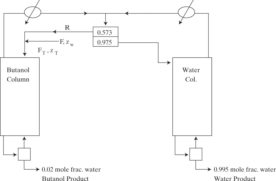
E3. Produce pure water from seawater by boiling it with n-decane vapor (see figure). This is sort of the reverse of steam distillation. Seawater is roughly 3.5 wt% salt, which can be approximated as NaCl. The feed is 1000.0 kg/h seawater at 30.0°C. The feed is heated with pure saturated n-decane vapor at 760.0 mm Hg. Most of the n-decane vapor condenses while the remainder is carried overhead with the water vapor. Pressure is 760.0 mm Hg. Recover 60.0% of the water as condensate.
a. Find the approximate still temperature.
b. Find the mol/h of n-decane carried over in the vapor.
Data: VP of n-decane: Example 8-2, VP of water: Problem 8.D10, MWwater = 18.016, MWNaCl = 58.45, MWC10 = 142.28, salt is nonvolatile. Water and n-decane are immiscible. NaCl dissolves only in water.
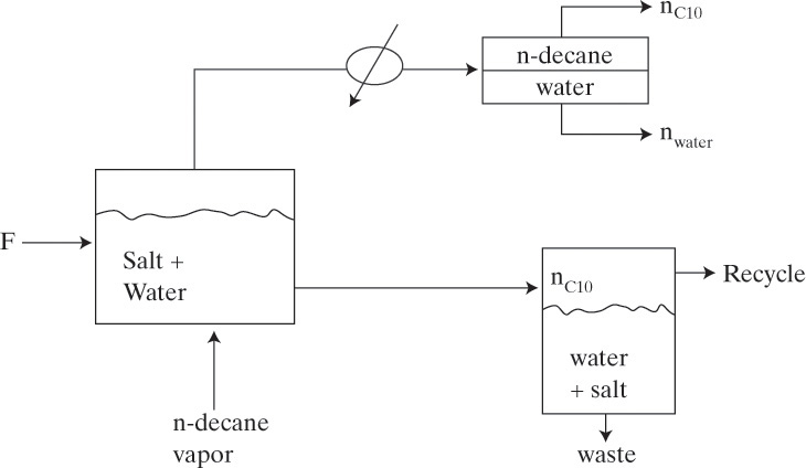
E4. Water containing 2.20 mol% n-butanol is sent at a rate of F = 105.0 kmol/h to an insulated tank. The feed is liquid at its boiling temperature. The entire apparatus is at 1.0 atm. Saturated pure vapor steam is sparged (bubbled in through liquid) into the tank at a rate of 8.0 kmol/h. The vapor exiting is sent to a condenser and then to a liquid-liquid separator. Organic product is withdrawn at P kmol/h. The water layer from the separator is refluxed to the tank. The tank is well mixed, and liquid is in equilibrium with vapor. Equilibrium data are in Table 8-2 (in Problem 8.D3), and CMO is valid. Find the mole fraction n-butanol in bottoms and the flow rates of bottoms, the vapor from the tank, the reflux, and P.
F. Problems Requiring Other Resources
F1.* A continuous, single-stage steam distillation is used to recover n-nonane (C9H20) from nonvolatile organics. Operation is at 1.0 atm, and the still will operate with liquid water present. If the still contains 99.0 mol% nonane in the organic phase (remainder is nonvolatiles), determine:
a. The temperature of still pot.
b. The moles of water vaporized per mole of nonane vaporized.
c. The moles of water condensed per mole of nonane vaporized for a liquid entering at still temperature.
d. Repeat parts a and b if the still pot contains 2.0 mol% nonane.
Data are available in Perry and Green (1984).
F2. Recover 90.0% of a gasoline component, n-nonane (C9H20), in the distillate from a nonvolatile mixture of oils, grease, and solids from a steady-state, single-stage steam distillation system operating with liquid water present at a total pressure of 102.633 kPa. The feed is 95.0 mol% n-nonane, enters at the temperature of the boiler, and is at a rate of 10.0 kmol/h. Find:
a. The bottoms mole fraction of n-nonane in the organic layer.
b. The still temperature.
c. The Kmol of nonane in distillate.
d. The Kmol of water in distillate.
e. The Kmol of water in bottoms.
Assume water and n-nonane are completely immiscible. Vapor pressure data for water are given in Problem 8.D10. Use a DePriester chart or Raoult’s law to obtain Kc9 (T, ptot). Then porg = (Kc9)(xc9,org)(ptot). Latent heat values are available in Perry’s and similar sources.
G. Computer Simulation Problems
G1. Separate a mixture of pyridine (C5H5N) and water, which form a homogeneous azeotrope, by using extractive distillation using bisphenol-A (C15H16O2) as the solvent. When finished, the system will look similar to Figure 8-13 with water as A product and pyridine as B product. The feed to column 1 is 200.0 kmol/h of a liquid at 80.0°C and 1.0 atm. Feed is 30.0 mol% pyridine and 70.0 mol% water. The makeup solvent is pure bisphenol-A at 1.0 atm and 100.0°C, and the recycle solvent is also cooled to 100.0°C with a heat exchanger operating at 1.0 atm. Produce a water product in D1 of 99.0 mol% water or slightly higher and a pyridine product in D2 of 98.0 mol% pyridine or slightly higher. Use NRTL for VLE correlation. Both columns have total condensers, kettle-type reboilers, pressure constant at 1.0 atm, and a saturated liquid reflux.
Column 1: N = 40, makeup solvent and, when connected, recycle solvent are both on stage 3 (N and solvent feed stages will not be changed), the feed is initially on stage 30 (all in Aspen notation), and reflux ratio = 0.1. Set an appropriate value for the distillate flow rate to produce pure water with no water in bottoms if separation were perfect.
Column 2: N = 8, feed is above stage 3 (all in Aspen notation), reflux ratio = 1.0. Set B2 initially to 1000.0 kmol/h. For the final design, stream B2 should have less than 10–5 mole fraction of water and pyridine. Note: N and the reflux ratio will not change.
The initial run will probably not give the desired purities. Find the optimum feed stage in column 1. Using this optimum feed stage and N1 = 40, increase the value of the solvent added by increments of 50.0 kmol/h until the desired purities of water and pyridine are obtained.
Estimate the desired makeup rate with an external balance. Once the system is operating at the desired makeup flow rate, if necessary to obtain the desired purities, make small adjustments in the following: D1, recycle flow rate B2, L/D in column 1, and makeup flow rate.
Report the following:
1. Final makeup solvent flow rate
2. Final value solvent recycle rate (B2) in kmol/h and L/D in column 1
3. Final values of flow rates D1, B1, and D2 in kmol/h
4. Mole fractions in stream D1
5. Mole fractions in stream D2
6. Mole fractions in stream B1
7. Mole fractions in stream B2 (solvent recycle stream)
8. Heat load in the cooler on the solvent recycle line in cal/s
G2. Your company plans to produce pure acetone from a mixture of acetone, methyl ethyl ketone, and methyl isobutyl ketone in an ordinary single-feed distillation column with a total condenser and a partial reboiler. The feed flow rate is 200.0 kmol/h; and feed mole fractions are acetone = 0.25, methyl ethyl ketone = 0.45, and methyl isobutyl ketone = 0.3. The feed can be made available at any desired pressure. Feed temperature is 75.0°C, D = 50.0 kmol/h, and it is an adiabatic column. Two senior engineers are arguing over the best column pressure. One claims that 1.0 atm is better and the other that 4.0 atm is better. They both agree that a NRTL VLE package is satisfactory. Use Aspen Plus to determine which pressure is better, and explain why it is better. There are at least two different approaches to solving this problem, and one is considerably less work than the other.
G3. We will use a system similar to Figure 8-4A, except both columns have direct reflux from their condensers in addition to reflux from a decanter. Distill a feed that is 17.0 mol% water and 83.0 mol% furfural (C5H4O2). The feed flow rate is 200.0 kmol/h and is at 42.0°C and 1.0 atm. Furfural-water forms a heterogeneous azeotrope. Use NRTL-RK for equilibrium. Bottoms from column 1 is a furfural product. The total condenser produces a saturated liquid, and saturated liquid distillate from column 1 is sent to the decanter. The water layer (liquid 1) from the decanter is fed to column 2. The decanter is adiabatic at 1.0 atm. Furfural (liquid 2) has a threshold of 0.5. The furfural layer is a feed (above) stage 2 (in Aspen notation) of column 1.
Distillation column 1 operates at a constant pressure of 1.0 atm. Column 1 has six stages (Aspen notation), a kettle reboiler, and a total condenser. The feed enters above stage 3, and the furfural layer from the decanter is fed above stage 2 (both Aspen notation). Use the total condenser to condense the distillate before it is sent to the decanter.
Distillation column 2 operates at a constant pressure of 1.0 atm. Column 2 has six stages (Aspen notation), a kettle reboiler, and a total condenser. The furfural layer from the decanter is fed above stage 2 (Aspen notation). The boilup rate in column 2 should initially be set to 4.0 kmol/h. Use the total condenser to condense the distillate and then send it as a second feed to the decanter. Reduce the reflux ratios in both columns to the final values of 0.01.
Once you have convergence and final reflux ratio values, change the boilup rate in column 2 to obtain products that are 99.5 mol% furfural or slightly higher and 99.0 mol% water or slightly higher. Report:
a. Final reflux ratio in column 1 and final reflux ratio in column 2
If these values are not 0.01 or less, you have not finished the problem.
b. Flow rates of the furfural product (kmol/h) and the water product (kmol/h)
c. Boilup rate in column 2 (column producing the water product) (kmol/h)
d. Mole fraction of the water furfural product and mole fraction of the furfural water product
e. Flow rate of column 1 distillate (column producing the furfural product) (kmol/h)
f. Column 1 condenser temperature (K) and reboiler temperature (K)
g. Outlet temperature of the decanter (K)
h. Molar ratio of the water phase/total liquid in the decanter
G4. The system water-acetonitrile (C2H3N) forms an azeotrope. This system can be separated using a two-pressure distillation system. Both columns have total condensers and kettle-type reboilers. Valid phases are vapor-liquid. Use NRTL for VLE data. The feed to the system is at 1.0 atm and 60.0°C. The feed is 15.0 mol% water and 85.0 mol% acetonitrile, and the feed flow rate is 200.0 kmol/h. This feed and the recycle stream labeled D2 in Figure 8-6 are input into column 1 above the same feed stage. Column 1 operates at 1.0 atm. As a start, column 1 has N = 15 and Nfeed = 8 (in Aspen notation) for both fresh feed and D2. This will provide more separation than necessary once a large enough value of D2 is determined. The molar reflux ratio for column 1 is 2.0. Set bottoms flow rate for column 1 at a value that will produce pure acetonitrile. Column 1 will eventually produce a bottoms product that is 99.5 mol% acetonitrile or higher. There is no need to change the specifications for column 1 (assuming they are input correctly).
Column 2 is at 200.0 torr. This column should eventually produce a bottoms product that is 99.5 mol% water or slightly higher. For column 2 use N = 14 (in Aspen notation) and feed on stage 7 (in Aspen notation). Initial molar reflux ratio = 2.0. Put a pump (discharge pressure of 1.0 atm and efficiencies for pump and driver of 1.0) between column 2 and column 1. Find the value of D2 (accurate to an increment of 10.0 in D2) that has column 1 meeting or slightly exceeding the desired purity of 99.5 mol% acetonitrile in bottoms and column 2 meeting or slightly exceeding the desired purity of 99.5 mol% water in bottoms. After the correct D2 has been determined, determine the lowest reflux ratio in column 2 (accurate to an increment of 0.1 in L/D) (N = 14 and feed on stage 7) as necessary to produce the desired bottoms product of 99.5 mol% water or very slightly higher. Report the following:
Column 1:
a. Bottoms product mole fraction acetonitrile
b. Distillate flow rate 9kmol/h) and desired bottoms flow rate (kmol/h)
c. Distillate mole fraction acetonitrile
Column 2:
a. Distillate flow rate (kmol/h) and molar reflux ratio
b. Bottoms product mole fraction water
c. Distillate mole fraction acetonitrile
G5. a. Aspen Plus automatically generates residue curves for ternary mixtures. Generate residue curve at 5.0 atm for a mixture of propane, n-butane, and n-pentane. Report the VLE correlation used.
b. To obtain some idea of what this means, simulate a column with a total condenser and kettle-type reboiler at 5.0 atm with 50 stages, a saturated liquid feed on stage 25 with F = 100.0 kmol/h, mole fractions of all three components = 0.333333, and initially far from total reflux (L/D = 0.999). Set D = 66.6667 to put pentane in bottoms. Generate a plot of liquid compositions versus stage location. To generate the plot, after the run, click the blue box with a checkmark. Then use the button with << to go to compositions. In the toolbar you will now see a button labeled Plot. Click this button and then click Plot Wizard in the menu. Click Next, click the plot type Comp, and click Next again. To plot all three components click the >> button. To plot liquid compositions, click the liquid button in middle of page. Click Next again and then Finish. This gives the desired plot. Print it, and label the conditions (L/D, mole fraction of feed, D, and N) on the plot. Note that complete separation is obtained.
c. Simulate the same system as in part b but with D = 33.3333. For the following, “essentially complete separation” means the propane mole fraction in distillate > 0.990. Is it possible to obtain essentially complete separation with
c1. L/D = 0.999, N = 100, and N feed = 50?
c2. N = 50 and N feed = 25 with L/D = 2.0?
c3. N = 10 and N feed = 5 with L/D = 2.0?
c4. N = 10 and N feed = 5 with L/D = 10.0?
c5. N = 6 and N feed = 3 with L/D = 50.0?
Print plots for cases with complete separation, and label the conditions on the plots.
d. The residue curve obtained implies that you can obtain pure propane or pure n-pentane for any feed composition by setting D appropriately and using a large enough L/D (> (L/D)min) and a large enough N (> Nmin). To convince yourself that this is true, try two different feed compositions, and show that essentially pure n-pentane can be obtained.
G6. To understand how two-pressure distillation works, in Lab 7 plot y-x diagrams (from Aspen Plus Analysis) for MEK versus water (plot MEK mole fractions) at 1.0 atm and for water versus MEK (plot water mole fractions) at 100.0 psia. For each diagram, mark the values for distillate and bottoms (MEK numbers for liquids on the 1.0-atm plot, and water numbers for liquids on the 100-psia plot). Then plot operating lines using the liquid and vapor flow rates found from the profiles (TPFQ tab). Note that the water concentration of D1 is the feed to the 100-psia plot. The net feed to the 1.0-atm plot is the average MEK concentration of the fresh feed plus stream D2. The distillation columns are forced to produce products very close to the azeotropic concentrations at both pressures.
H. Computer Spreadsheet Problems
H1. Generation of distillation and residue curves for systems with constant relative volatility is fairly straightforward and an excellent learning experience. Generate distillation curves in Figure 8-7 for a benzene (A), toluene (B), and cumene (C) system with αAB = 2.4, αBB = 1.0, and αCB = 0.21. Operation is at total reflux.
a. * Mole fraction of A in the reboiler is 0.006735, and mole fraction of B is 0.003469.
b. * Mole fraction of A in the reboiler is 0.001, and mole fraction of B is 0.009.
c. Mole fraction of A in the reboiler is 0.0003, and mole fraction of B is 0.0097.
Remember Σ (mole fractions in the still pot) = 1.0. *Solution is shown in Figure 8-7.
H2. Generate residue curves for the benzene (A), toluene (B), and cumene (C) system with αaB = 2.4, αBB = 1.0, and αCB = 0.21. Mole fractions of A and B in the still pot are 0.990 and 0.001, respectively. Compare your results with the distillation curves in Figure 8-7. Remember Σ (mole fractions in the still pot) = 1.0.
H3. Usually, relative volatilities are not constant, and determination of the residue curve requires a bubble-point calculation to determine the temperature, T, and the vapor mole fractions at each time used to integrate Eq. (8-28). A bubble-point calculation is illustrated in Example 5-3 for light hydrocarbons. K values for these compounds can be determined from Eq. (2-28) with constants tabulated in Table 2-3. Develop a spreadsheet that can be used to determine residue curves for any three of the following light hydrocarbons: i-butane, n-butane, i-pentane, n-pentane, and n-hexane. Note: If Euler’s method, Eq. (8-29), is used, tolerance on the sum of yi,k values must be quite small (e.g., E-9). Find the residue curve for
a. n-butane, i-butane, and n-pentane.
b. i-pentane, n-pentane, and n-hexane.
c. any other combination of interest.
Chapter 8 Appendix A. Simulation of Complex Distillation Systems
Although the Aspen Plus simulator is referred to, other process simulators can be used. The three problems in this appendix all employ recycle streams. The procedures shown here to obtain convergence are all forms of stream tearing. Since these are not the only methods that will work, you are encouraged to experiment with other approaches. If problems persist while running the simulator, see Appendix A: Aspen Plus Separations Troubleshooting Guide, at the end of the book.
VLE for the very nonideal systems studied in this chapter may not fit well with any of the VLE correlations in Aspen Plus if the parameters embedded in Aspen Plus are used. An alternative is to use Aspen Plus to fit parameter values to give the best fit to VLE data. This procedure is explained in Appendix B at the end of the book.
Lab 7. Pressure-Swing Distillation For Separating Azeotropes.
Goal:
Use Aspen Plus simulation to explore application of distillation at two pressures as a method to separate azeotropic mixtures.
• Review computer Labs 1 to 6 as needed.
• Read Section 8.4.
The arrangement of columns shown in Figure 8-6 (or the very similar arrangement in which feed is input into the higher pressure column 2) can be used to separate azeotropes if azeotrope concentration shifts significantly when pressure is changed.
Use Strongly non-ideal for convergence of both columns.
I. Set up the system, flowchart, and specifications:
1. We want to separate a fresh feed that is 60.0 mol% water and 40.0 mol% methyl ethyl ketone (MEK), CH3COC2H5. Note: Input the component name as methyl-ethyl-ketone. Although not a perfect fit, the Wilson equation gives reasonable VLE data. Use Analysis to look at T-y,x, tabular data, and y-x plots at 1.0 atm and at 100.0 psia. Record the mole fraction of water of the azeotrope at both pressures. Feel free to look for better VLE packages.
2. When you draw the flowchart (see Figure 8-A1), put a pump (select under pressure changers) on the distillate line going from column 1 that becomes the feed to column 2. The resulting flowsheet should be similar to Figure 8-A1.
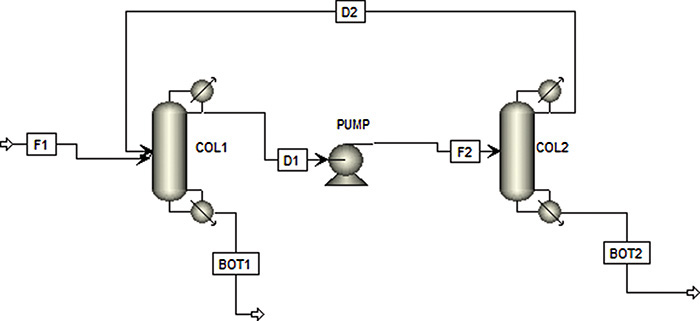
3. The feed is 60.0 mol% water and 40.0 mol% MEK and is a saturated liquid at 1.0 atm. The fresh feed rate to column 1 is 100.0 kmol/h. Column 1 operates at 1.0 atm. Start with N = 10, both feeds are liquid on Nfeed = 5, and L/D = 1.0 in column 1. Distillate is a saturated liquid. Use a total condenser and a kettle-type reboiler. We want products that are ≥ 99.0% purity. Specify the bottoms flow rate of column 1 = 60.0 kmol/h. Set convergence at 75 iterations.
4. Column 2 is at 100.0 psia and has a total condenser, a saturated liquid distillate, and a kettle-type reboiler. Start with N = 15 and the feed at Nfeed = 7, with L/D = 2.0. Set convergence at 75 iterations. Do NOT specify bottoms in column 2. (Why not?) Instead specify the flow rate of recycle stream D2.
5. Set pump efficiency = 1.0 and discharge pressure = 100.0 psia.
II. Runs
6. First, in column 2 start with a distillate rate D2 = 100.0 kmol/h, and run the simulation. If you look at all items list, the red X for results for the second column means there was an error in the simulation. In addition, control panel reports a severe error: column not in mass balance. Also, look at Report for all three blocks. Note that there is an error in column 2’s calculation.
7. To obtain valid results, reduce the distillate rate to D2 = 20.0 kmol/h, run the simulation, and look at the composition of the bottoms products. There is some separation, but the purity requirements are not satisfied. Increase D2 in steps (i.e., 30, 40, 50, 60, 70 kmol/h, and so forth) until the purity requirements are met. If you do not step up, the Aspen Plus control panel will report errors. Note that B2 in column 2 = 40.0 kmol/h every time even though you did not specify it (Why?). Continue increasing D2 until both purities are ≥99%. Use the lowest D2 (within a flow rate of +1.0 kmol/h) that gives the desired purities.
8. Once an appropriate value for D2 is found, firm up the designs for both columns. For example, in column 2 reduce the reflux ratio to 1.75, 1.5, 1.25, and 1.0. The reflux ratio has only a small effect, although at a value of 1.0, the purity requirement for the MEK product may not be met.
9. At a reflux ratio = 1.0 with N2 = 15, find the optimum feed stage. Record the optimum feed stage location and the purities of both bottoms products. If the purity requirements are satisfied, reduce the reflux ratio further. Once the purity requirement is not satisfied, find the optimum feed stage again (it may shift a bit). The goal is to have a low reflux ratio with N2 = 15 and still satisfy the purity requirements for both products.
10. If you have time, a similar analysis can be done for column 1. Complete optimization of the system requires an economic analysis (see Chapter 11).
III. Tray sizing
11. After you are happy with the design, run it one more time to size the trays for both columns. Use sieve trays with the Fair flooding calculation method in the Design tab and default values for the other variables. Record distillate flow rates, heat loads, and the column diameters.
12. Why are distillate flow rates so large? Note that these large distillate flow rates make column diameters and heat loads large for this very modest feed rate. These large recycle rates and hence large diameters and heat loads make this design economical only when the shift of the azeotrope with pressure is rather large. MEK and water are separated commercially with two-pressure distillation.
Before going to Part IV, check your values of D2, (L/D)col 2, and the optimum feed stage in column 2 with your instructor.
IV. Plotting McCabe-Thiele Diagram from Aspen Plus Simulation and Assignment
While in the lab, print out the y-x graphs that you will need to solve Problem 8.G6 (MEK versus water [plot MEK mole fractions] at 1.0 atm and water versus MEK [plot water mole fractions] at 100.0 psia). In addition, print the tables that give liquid and vapor flow rates for both columns. Read Problem 8.G6 before you close Aspen Plus to be sure you have all values needed.
Lab 8. Binary Distillation of Systems with Heterogeneous Azeotropes
Goal:
Use Aspen Plus simulation to explore separation of binary systems that have a heterogeneous azeotrope.
The purpose of this lab is to design systems similar to Figures 8-3A and 8-4A for separating n-butanol and water.
Preparation
• Review computer Labs 1 to 6 as needed.
• Review convergence procedures for systems with loops (Lab 7).
• Carefully review convergence procedures in Figure 6-1.
• Read Section 8.7.
Preliminary
1. Open a new, blank file. Under Setup, set units to MET and valid phases as Vapor-Liquid-Liquid. List n-butanol and water as the components.
2. Finding a suitable VLE model for heterogeneous azeotropes is a challenge. NRTL-RK was the best model of the half dozen I tried. NRTL-RK fits the vapor composition of the azeotrope and the liquid composition of the water phase quite well (see Table 8-2 in Problem 8.D3) but misses a bit on the butanol phase composition. (Feel free to fit the NRTL-RK constants using the method in Appendix B at the back of the book.)
3. Use Analysis to look at the T-y,x and y-x plots. Compare with the data. Remember to allow Vapor-Liquid-Liquid as the phases in Analysis.
Part I. Single-Column System (Figure 8-3A)
4. In simulation mode draw a flow diagram. Use a total condenser. The distillate product is a liquid, and this line is connected to the decanter (or liquid-liquid settler) feed (listed in Model Palette under Separators). The hydrocarbon layer from the decanter (first phase) should be connected to the distillation column feed. The aqueous layer (second phase) from the decanter is the water product. The flowsheet for the one-column system is shown in Figure 8-A2. Note that the Aspen Plus column in Figure 8-A2 does not look exactly like the arrangement in Figure 8-3A. We are using the condenser on the column to condense the liquids. We will use specification sheets to make the system behave like Figure 8-3A.
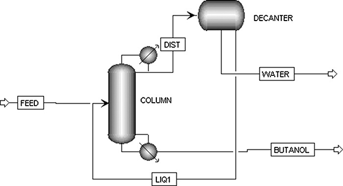
5. The feed is 100.0 kmol/h of a saturated liquid feed at 1.0 atm pressure. The feed is 78.0 mol% n-butanol and 22.0 mol% water.
6. Column: Calculation Type: Select equilibrium from menu.
a. Start with the number of stages N = 10.
b. Use a total condenser and a kettle-type reboiler.
c. Select Vapor-Liquid for valid phases.
d. Select convergence as the strongly nonideal liquid.
e. Set the reflux ratio to 0.5. We do not really want to reflux from the condenser, but we do want to take our reflux from the decanter; however, if you try setting the reflux ratio to 0.0, Aspen Plus will not run. Reduce the reflux ratio in a few steps down to about 0.025. This ratio is small enough that results will be very close to using only reflux from the decanter phases. If you do not do this in steps, the condenser will dry up, and the run will have errors. Pamper Aspen Plus, and make it happy! After you finish the lab, you might try reinitializing, and see what happens if you set the reflux ratio to 0.025. Results when the column is dried up are not useable.
f. Specify a bottoms flow rate that will give you the desired purity of the butanol product (0.990 or higher mole fraction). Purity of the water product from the decanter depends on the VLE correlation used. Initially, use the value from Table 8-2 and then correct it once you have the decanter results. The mass balance to calculate the bottoms flow rate has to be accurate.
g. Initially, specify the feed location NF = 5 as a liquid.
h. Specify that the line from the decanter is input in the distillation column at N = 2 as a liquid.
i. Operate at a pressure of 1.0 atm.
j. If you have convergence difficulties, first verify that you checked Strongly non-ideal liquid for the column. If you still have difficulties, in the convergence section of the column block, set the number of iterations to 75. Higher values usually do not help.
7. Decanter. Pressure is 1.0 atm, and the heat duty is 0.0 (adiabatic). The key component for the second phase is water, and set the threshold at ∼0.7 (equilibrium data show the highest water content in the organic phase is <0.6). If you have difficulty with decanter convergence, first set the convergence at 75 iterations. If that does not help, reduce the decanter’s error tolerance.
8. Run the simulation. If the water product purity is different than the value used for mass balance to determine the bottoms flow rate, redo the mass balance. Run the simulation again with the revised bottoms value.
9. Record mole fractions, temperatures, and flow rates (kmol/h) of the butanol and water product streams, the hydrocarbon layer refluxed to the column from the decanter (LIQ1 in Figure 8-A2), and distillate.
Part II. Two-Column System (Figure 8-4A)
For Part II the purity of both products is 99.0 mol% or higher.
10. Recalculate the bottoms flow rate for the distillation column based on the new water product purity. Adjust the first column’s condition.
11. Modify your flowsheet to include a stripping column (Figure 8-4A), except use the column condenser to produce a liquid distillate. Your flowsheet should be similar to Figure 8-A3.
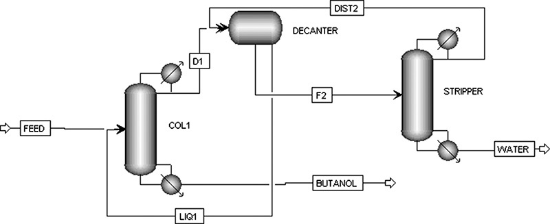
12. Stripping column specifications: Calculation Type: Select equilibrium from the menu.
a. Initially set the number of stages to N = 10.
b. Use a total condenser and a kettle-type reboiler.
c. Select Vapor-Liquid for the valid phases.
d. Select convergence as Strongly non-ideal liquid.
e. Set the reflux ratio to 0.5. Reduce the reflux ratio in a few steps down to about 0.025.
f. Set the boilup rate to 1.0 kmol/h in the stripping column. This is rate, not boilup ratio.
g. The line from the decanter should be input as feed on stage 2 (first actual stage in the column). If you have convergence difficulties, see instruction step 7.
h. Pressure is 1.0 atm.
13. Run the simulation for a two-column system. If one or both columns are not producing products as pure as required, increase the boilup rate in the stripper modestly in increments of 0.2 kmol/h until both products meet the purity specifications.
14. If the butanol product is purer than necessary, this implies column 1 can have fewer stages and/or a lower boilup ratio. However, before changing the conditions, save your results, and note that there is an inherent difficulty in the set of specified variables for the flowsheet in Figures 8-A2 and 8-A3. The loop from Col-1 to the Decanter and back to Col-1 via the HC-Layer does not have control on flow rates. (The other loop from the Stripper to the Decanter and back does because the boilup rate in column 2 is specified.) Thus, it is possible for the flow rates of Distil-1 and HC-Layer to become very large. This will happen if the number of stages in Col-1 are reduced drastically. The cure is to set a flow rate that will control this loop; however, since the number of variables you can specify is set, another variable has to be made free. A method that works once Aspen Plus is giving good results is to set the reflux ratio (0.025) and the boilup rate in Col-1 (use the value from the run with 10 stages and Nfeed = 5 with bottoms in Col-1 specified). To be sure this works, repeat the previous run but with the boilup rate in Col-1 replacing the specification of the bottoms rate. Then reduce the number of stages and the feed location. Increase Col-1 boilup rate by a maximum of 10.0% to obtain the desired separation. If there are convergence difficulties as you do this, try decreasing the error tolerance for each column to 1.0 E-5. Also try increasing the number of maximum flowsheet iterations in the Wegstein method to 75 (below Block, Utilities, and Reactions in Aspen Plus, click Convergence→Conv Options→Methods→Wegstein tab→Convergence Parameters).
15. Report your results for the two-column system: list the number of stages in both columns, optimum feed locations, boilup rates in both columns, and product purities.
16. When done, make the two-column system not converge! Return to the original number of stages, the original feed location, and the original specification of the bottoms flow rate in the butanol column. Increase the boilup rate in the water stripper to 10.0 kmol/h, and run the simulation. Messages in the control panel, in the run summary, and the reports for the blocks all state there is a problem. However, the stream reports do not state there is a problem. Do NOT save runs that do not converge.
Lab 9. Simulation of Extractive Distillation
Goal:
Use Aspen Plus simulation to explore the application of extractive distillation as a method to separate azeotropic mixtures.
Preparation:
• Review computer Labs 1 to 6 as needed.
• Review the convergence procedures for systems with loops (Labs 7 and/or 8).
• Carefully review the convergence procedures in Figure 6-1.
• Read Section 8.6.
This assignment is more prescriptive and involves less exploration than other labs since convergence can be difficult with extractive distillation. The basic algorithm (Figure 6-1) assumes the concentration loop will have little effect on the other loops. Extractive distillation systems have very nonideal VLE, and concentrations have a major effect on K values. As always with Aspen Plus, it may be possible to obtain convergence by starting with a set of conditions that converges and slowly changing the variable of interest (e.g., D) to approach the desired value. When you have a convergence problem, first reread the instructions to be sure you have properly set convergence parameters. Next, try increasing the number of iterations in the block (your distillation column) convergence by 1 (this is done so that Aspen Plus will run again) and then run it again. Second, a modest reduction in error tolerance in the convergence may help—then run it again. Fourth, return to a condition that converged previously and run it. If this condition does not run, reinitialize Aspen Plus, and run the known conditions that converged. Once Aspen Plus is running, work your way toward the desired condition by changing the desired variable (e.g., D) by modest amounts.
Use Strongly non-ideal for convergence of both columns.
Standard convergence will not work.
I. Desired specifications
In Figure 8-13 the A product will be the ethanol product, and the B product (distillate from column 2) will be water.
A. The ethanol product must be at least 99.75 mol% ethanol (this exceeds the requirements for ethanol used in gasoline).
B. The bottoms product from column 1 should have less than 0.009 mol% ethanol. This number is low to increase the recovery of ethanol.
C. The distillate from column 2 should contain less than 0.01 mol% ethylene glycol. This value is low to reduce the biological oxygen demand (BOD) of the water.
D. The bottoms product from column 2 should contain less than 0.01 mol% water since water in this stream will probably exit in the ethanol product when the solvent is recycled.
II. Set up system and flowchart
1. In Setup the valid phases are Vapor-Liquid. To use extractive distillation to break the ethanol-water azeotrope, input the components ethanol, water, and ethylene-glycol. For VLE use NRTL. After running property/analysis setup, click Residue Curves (right side of the Home toolbar) for the system at a pressure of 1.0 atm. Make the water component 1, the ethylene glycol component 2, and the ethanol component 3 (you may need to override Aspen Plus to do this). Run the analysis with 10 to 15 curves. Compare your result with Figure 8-14.
2. In Simulation mode draw the two-column system shown in Figure 8-13, but do not connect the solvent recycle (leave it as a product initially). Both columns should be drawn with liquid distillate products. The flowsheet will be similar to Figure 8-A4, except the solvent recycle is not connected.
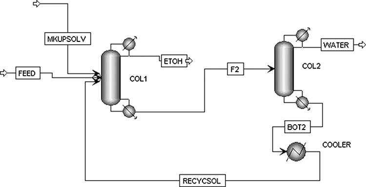
3. The feed to column 1 is 100.0 kmol/h of a saturated liquid at 1.0 atm pressure that is 74.0 mol% ethanol and 26.0 mol% water.
4. The makeup solvent is pure ethylene glycol at 1.0 atm pressure. However, initially use a makeup solvent that is close to the expected concentration of the recycle solvent. That is, the solvent stream should be 99.99 mol% ethylene glycol and 0.01 mol% water. Use a solvent temperature of 80.0°C to approximately match the temperature of the solvent feed stage (NS = 5) in column 1. Use an initial solvent rate of S = 52.0 kmol/h.
5. Column 1. Calculation Type: Select equilibrium from the menu.
a. Start with the number of stages at N1 = 50.
b. Use a total condenser.
c. Select Vapor-Liquid for valid phases.
d. Select the convergence as Strongly non-ideal liquid.
e. Use the external reflux ratio in column 1 of L/D = 1.0. (Normally L/D would be optimized, but to save time leave it constant.) The reflux is returned as a saturated liquid.
f. Specify the distillate flow rate that will give you the desired purity of ethanol product and the desired ethanol mole fraction in bottoms product (do external balances). The mass balance to calculate distillate flow rate has to be accurate.
g. Initially, specify the feed location as NF1 = 23.
h. The solvent is treated as a second feed to column 1. In the flow diagram, use the feed port to add a solvent feed to the column. Then specify its location (NS = 5) in the Specifications for the column Block in the Streams tab.
i. Operate at a pressure of 1.0 atm.
j. In the Simulation All Items menu on the left-hand side of the screen, click the arrow next to the block for distillation column 1. In the subheadings for this block click the arrow next to Convergence and then click the sub-subheading Convergence. In the Basic tab under Basic convergence are menus In the menu for Maximum iterations increase the number to 75.
This set of conditions should remove sufficient ethylene glycol from distillate to produce an ethanol of suitable purity (check to make sure that this happens).
6. Column 2. In the flow diagram the feed to column 2 is the bottoms from column 1.
a. Calculation Type: Select equilibrium from menu.
b. Start with the number of stages as N2 = 50 to find (L/D)min for column 2.
c. Use a total condenser.
d. Select Vapor-Liquid for the valid phases.
e. Select the convergence as Strongly non-ideal liquid.
f. Initially use an external reflux ratio in column 2 of L/D = 1.0.
g. Specify the bottoms flow rate that will give you the desired purity of the distillate and bottoms products (do external balances for the system with makeup solvent = 52.0 and no recycle of solvent). The mass balance to calculate bottoms flow rate has to be accurate.
h. Initially, specify the feed location as NF2 = 25.
i. Operate at a pressure of 1.0 atm.
j. In the convergence section block for column 2 (see item 5j) set the number of iterations to 75.
7. Run the Simulation. If you do not satisfy product specifications (ethanol product is 99.75 mol% ethanol or higher; bottoms column 1 is less than 0.009 mol% ethanol; distillate product column 2 is less than 0.01 mol% ethylene glycol) you need to adjust your specified distillate and bottoms flow rates in columns 1 and 2, respectively. If your ethanol distillate mole fraction is >0.975, but the ethanol bottoms mole fraction >0.00009, the cause may be a distillate flow rate that is too low. Exceeding purity requirements is okay at this point, since the system is not coupled. Do not go to step 8 until you satisfy or exceed the specifications.
8. Design column 1. Find the approximate optimum feed stage and the lowest total number of stages that will do the desired separation. Start by keeping NF1 fixed while you reduce N (total number of stages in column 1) to approximately obtain the desired bottoms and distillate concentrations. Then vary NF1 to find the optimum feed stage. Once you have the optimum feed stage, try reducing N more. Low values of the feed stage (e.g., NF1 = 10) will probably not converge. Thus, start with a high number for the feed stage location and reduce NF1.
9. Design column 2. The feed to column 2 is the bottoms from column 1. It is a saturated liquid at 1.0 atm. Very small adjustments in the bottoms flow rate of column 2 may be necessary to meet specifications. Find an approximate (L/D)min (N2 = 50 and NF2 = 25 is sufficient; start with L/D = 1.0 and move down). Column 2 is quite simple, and a low value of L/D works. Aspen Plus may have convergence problems near the value of (L/D)min. Try increasing the number of runs in the convergence by 1 (to 76), and run it again. Sometimes Aspen will converge. Do runs with L/D > (L/D)min where the purity is better than required and runs where the purity is less than required, which means L/D < (L/D)min. Then approximate (L/D)min.
10. Operate column 2 with L/D = 1.15(L/D)min, and find the optimum feed stage location and the lowest value of N2 that gives the desired separation (start with N2 = 20 and NF2 = 10).
11. Heat exchanger. Eventually we will connect the solvent recycle loop from column 2 to column 1. First, include a heat exchanger to cool the solvent. If you do not cool the solvent, column 1 will not work after you connect the solvent recycle loop. (Why not?) (To put a heat exchanger in the solvent recycle line, go to Heat Exchangers, and put a Heater—used as a cooler in this case—in your flowsheet. Then left-click on the solvent stream, and right-click on Reconnect Destination. Connect the solvent stream to the heat exchanger inlet arrow. Click Next. In the heat exchanger window use 80.0°C, pressure = 1.0 atm, valid phases are liquid only.) To check that Heater is hooked up properly, try a run.
12. Close the loop. Connect the line leaving heater to column 1 (use the reconnect destination, and connect to the column 1 feed port). In the table of input conditions, list the solvent makeup stream and the recycle line at the same stage (NS = 5). Your flowsheet should be very similar to Figure 8-A4.
13. Calculate the solvent makeup flow rate at steady state. To calculate the makeup solvent flow rate that you eventually want to use, do an external mass balance around entire system:
pure solvent makeup flow rate = solvent out in A product + solvent out in B product
The resulting solvent makeup flow rate will be extremely small since losses of solvent are small (after all, no one wants to drink ethylene glycol with their alcohol or their water). If you immediately use this value of solvent makeup as a feed to the system, Aspen Plus will not converge.
14. Reduce the solvent makeup flow rate in steps. Start with the value you were using before closing the loop, and rapidly decrease it (say by factors of roughly 5 or 10). Until the solvent makeup stream is at the desired value from the external mass balance, extra ethylene glycol will exit with distillate (water product) from column 2. This occurs because the bottoms flow rate in column 2 is specified, and the only place for extra ethylene glycol to go is with the distillate from column 2. (This is why you must set the bottoms rate in column 2. If you set the distillate rate in column 2, there is no place for the extra ethylene glycol to go, and the system will not converge.) Ignore the values of the distillate flow rate and the compositions from column 2 until you use the makeup solvent rate that satisfies the steady state external balance. Once you are close to the correct makeup flow rate, change it to pure ethylene glycol. The system should now be similar to Figure 8-A3.
If for some reason (not recommended) you have to uncouple the recycle loop, remember to reset the makeup flow rate to the desired value.
15. If necessary, make minor adjustments in stages, flows, or reflux ratios to achieve the desired purities.
16. When everything is working set up tray sizing for both columns (sieve trays at 80.0% of flooding using the Fair flooding correlation with default values for the other variables).
17. As a minimum, record the following: mole fractions of the two products and the two bottom streams; heat duties of the two condensers, the two reboilers, and the heat exchanger; flow rates of all streams in the process; L/D in each column; N and feed locations in each column; diameter of each column; and temperatures of the reboilers and condensers.
Chapter 8 Appendix B. Spreadsheet for Residue Curve Generation
Calculation of a residue curve for constant relative volatility using Euler’s method is illustrated in Example 8-3. This calculation is repeated a very large number of times. A spreadsheet with a VBA program incrementing the step number is a convenient method to do the repeated calculations. A spreadsheet with numbers in the cells is shown in Figure 8-B1, with formulas in the cells is shown in Figure 8-B2, and the VBA program is shown in Table 8-B1.
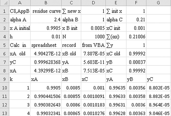
FIGURE 8-B1. Spreadsheet for constant α calculation of residue curve. Calculations continue to k = 1000.0.