Chapter 11. Determining Headroom for Applications

Knowing the place and the time of the coming battle, we may concentrate from the greatest distances in order to fight.

—Sun Tzu

The last thing that anyone wants is for his or her company to be remembered for or associated with some type of failure. The authors of this book remember this feeling all too well from our early days at eBay, when the company was the poster child for technical glitches. More recently, at least into 2012, the best-known story of this type has been about Twitter and the infamous “Fail Whale.” In the early days of Twitter, when it would experience significant problems, the service would display the picture of a whale being lifted out of the water by tiny birds, along with the statement “Twitter is over capacity.” This event seemed to happen so often that the Fail Whale took on a following all its own, with people making money selling clothing with the image of the giant mammal and tiny birds.¹ Failing for reasons of under-capacity, as the Fail Whale’s statement would seem to imply, is completely avoidable with the right processes and appropriate funding. Unfortunately, besides giving Twitter a great deal of unwanted press, this type of event remains one of the most common failures we see in our consulting practice. And for the record, it’s happened to us as well.

1. Sarah Perez. “How an Unknown Artist’s Work Became a Social Media Brand Thanks to the Power of Community.” July 17, 2008. http://readwrite.com/2008/07/17/the_story_of_the_fail_whale.

This chapter walks you through the process of determining headroom for your product. We start with a brief discussion of the purpose of headroom and an exploration of where it is used. Next, we describe how to determine the headroom of some common components found in systems. Lastly, we discuss the ideal conditions that you want to look for in your components in terms of load or performance.

For instance, annual budget planning should be informed by an understanding of your product headroom. To understand how much equipment (e.g., network gear, compute nodes, database licenses, storage) you need to buy, you must first understand both the forecasted demand and your current capacity (or headroom). Without this understanding, you are just making an educated guess with equal probability of over-purchasing or (gasp) under-purchasing. Many organizations do a rough, back-of-the-envelope calculation by saying, for example, they grew x% this year and spent $y, so therefore if they expect to grow x% again next year, they should spend $y again. Although this passes as a planned budget in many organizations, it is guaranteed to be wrong. Not taking into account different types of growth, existing headroom capacity, and optimizations, there is no way your projections could be accurate other than by pure luck.

Hiring is another area in which headroom calculations are useful. Without understanding headroom and future product growth expectations, how do you know how many people with each skill set (e.g., software developers, database administrators) you will need in your organization? If you understand that you have plenty of headroom on your application servers and on your database but you are bumping up against the bandwidth capacity of your firewalls and load balancers, you might want to add another network engineer to the hiring plan instead of another systems administrator.

Headroom is also useful in product planning. As you design and plan for new features during your product development life cycle, you should be considering the capacity requirements for these new features. If you are building a brand-new service, you will likely want to run it on its own pool of servers. If this feature is an enhancement of another service, you should consider its ramifications for the headroom of the current servers. Will the new feature require the use of more memory, larger log files, intensive CPU operations, the storage of external files, or more SQL calls? Any of these factors can impact the headroom projections for your entire application, from network to database to application servers.

Understanding headroom is critical for scalability projects. You need a way to prioritize your scalability and technical debt projects. In the absence of such a prioritization mechanism, “pet projects” (those without clearly defined value creation) will bubble to the top. The best (and, in our mind, only) way of prioritizing projects is to use a cost–benefit analysis. The cost is the estimated time in engineering and operations effort to complete the project. The benefit is the increase in headroom or scale that the projects will bring—sometimes it is measured in terms of the amount of business or transactions that will fail should you not make the investment. After reading through the chapter on risk management, you might want to add a third comparison—namely, risk. How risky is the project in terms of impact on customers, completion within the timeline, or impact on future feature development?

By incorporating headroom data into your budgeting, planning, and prioritization decisions, you will start making much more data-driven decisions and become much better at planning and predicting.

The first step in the headroom process is to identify the major components of the product. Infrastructure such as network gear, compute nodes, and databases needs to be evaluated on a granular level. If you have a service-oriented architecture and different services reside on different servers, treat each pool separately. A sample list might look like this:

• Account management services application servers

• Reports and configuration services application servers

• Firewalls

• Load balancers

• Bandwidth (intra- and inter-data center or colocation connectivity as well as public transit/Internet links)

• Databases, NoSQL solutions, and persistence engines

After you have reduced your product to its constituent components, assign someone to determine the usage of each component over time, preferably the past year, and the maximum capacity in whatever is the appropriate measurement. For most components, multiple measurements will be necessary. The database measurements, for example, would include the number of SQL transactions (based on the current query mix), the storage, and the server loads (e.g., CPU utilization, “load”). The individuals assigned to handle these calculation tasks should be the people who are responsible for the health and welfare of these components whenever possible. The database administrators are most likely the best candidates for the database analysis; the systems administrators would be the best choice to measure the capacity and usage of the application servers. Ideally, these personnel will use system utilization data that you’ve collected over time on each of the devices and services in question.

The next step is to quantify the growth of the business. This data can usually be gathered from the general manager of the appropriate business unit or a member of the finance organization. Business growth is typically made up of many parts. One factor is the natural or intrinsic growth—that is, how much growth would occur if nothing else was done to the product or by the business (no deals, no marketing, no advertising, and so on) except basic maintenance. Such measurements may include the rate at which new users are signing on and the increase or decrease in usage by existing users. Another factor is the expected increase in growth caused by business activities such as developing new or better features, marketing, or signing deals that bring more customers or activities.

The natural (organic) growth can be determined by analyzing periods of growth without any business activity explanations. For instance, if in June the application experienced a 5% increase in traffic, but there were no deals signed in the prior month or release of customer-facing features that might explain this increase, we could use this amount as our organic growth. Determining the business activity growth requires knowledge of the planned feature initiatives, business department growth goals, marketing campaigns, increases in advertising budgets, and any other similar metric or goal that might potentially influence how quickly the application usage will grow. In most businesses, the business profit and loss (P&L) statement, general manager, or business development team is assigned goals to meet in the upcoming year in terms of customer acquisition, revenue, or usage. To meet these goals, they put together plans that include signing deals with customers for distribution, developing products to entice more users or increase usage, or launching marketing campaigns to get the word out about their fabulous products. These plans should have some correlation with the company’s business goals and can serve as the baseline when determining how they will affect the application in terms of usage and growth.

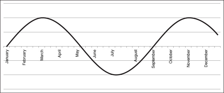
After you have a very solid projection of natural and human-made growth, you can move on to understanding the seasonality effect. Some retailers receive 75% of their revenue in the last 45 days of the year due to the holiday season. Some experience the summer doldrums, as people spend more time on vacation and less time browsing sites or purchasing books. Whatever the case for your product, you should take this cycle into account to understand what point of the seasonality curve you are on and how much you can expect this curve to raise or lower demand for your products and services. If you have at least one year’s worth of data, you can begin projecting seasonal differences. The way to accomplish this is to strip out the average growth from the numbers and see how the traffic or usage changed from month to month. You are looking for a sine wave or something similar to Figure 11.1.

Figure 11.1 Seasonality Trend

Now that you have seasonality data, growth data, and actual usage data, you need to determine how much headroom you are likely to retrieve through your scalability initiatives next year. Similar to the way we used the business growth for customer-facing features, you need to determine the amount of headroom that you will gain by completing scalability projects. These scalability projects may include splitting a database or adding a caching layer. For this purpose, you can use various approaches such as historical gains from similar projects or multiple estimations by several architects, just as you would when estimating effort for story points (similar to the practice of “pokering” in Agile methods). When organized into a timeline, these projects will indicate a projected increase in headroom throughout the year. Sometimes, projects have not been identified for the entire next 12 months; in that case, you would use an estimation process similar to that applied to business-driven growth. Use historical data to estimate the most likely outcome of future projects weighted with an amount of expert insight from your architects or chief engineers who best understand the system.

The last step is to bring all the data together to calculate the headroom. The formula for doing so is shown in Figure 11.2.

Figure 11.2 Headroom Equation

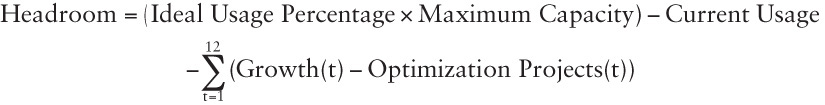
This equation states that the headroom of a particular component of your system is equal to the ideal usage percentage of the maximum capacity minus the current usage minus the sum over a time period (here it is 12 months) of the growth minus the optimization. We will cover the ideal usage percentage in the next section of this chapter; for now, let’s use 50% as the number. If the headroom number is positive, you have enough headroom for the period of time used in the equation. If it is negative, you do not.

Let’s practice using this headroom calculation process. Imagine you are asked to calculate the headroom of a database in terms of SQL queries within your environment. You determine that, assuming a query mix (reads, writes, use of indexes, and so on) similar to what you have now, you can service a total of 100 queries per second. You arrive at that estimate by looking at the largest constraining factors within the server and storage arrays upon which the database is deployed. Today the database processes 25 queries per second during peak utilization. Based on information you receive from your business unit leader, you determine that organic and business-driven growth will likely result in an additional 10 queries per second over the course of the year during peak transaction processing time. As a result of examining past transaction rates over the course of the last year, you know that there is a great deal of seasonality in your business and that peak transaction times tend to happen near the holiday season. You and your team further decide that you can reduce the queries per second on the database by 5 through a combination of query elimination and query tuning.

To evaluate your headroom, you plug these numbers into the headroom equation shown in Figure 11.2, using 0.5 as the ideal usage percentage. This results in the following expression, where q/s stands for queries per second and tp is the time period—which in our case is 1 year or 12 months:

Headroom q/s = 0.5 × 100 q/s – 25 q/s – (10 – 5) q/s/tp × 1 tp

Reducing this equation results in the following:

Headroom q/s = 50 q/s – 25 q/s – 5 q/s = 20 q/s

Since the number is positive, you know that you have enough headroom to make it through the next 12 months.

But what does the headroom number 20 q/s mean? Strictly speaking, and relative to your ideal usage factor, you have 20 queries per second of spare capacity. Additionally, this number, when combined with the summation clause (growth, seasonality, and optimization over the time period), tells the team how much time it has before the application runs out of headroom. The summation clause is shown in Figure 11.3.

Figure 11.3 Headroom Time Equation

Solving this equation, Headroom Time = 20 q/s ÷ 5 q/s/tp = 4.0 tp. Because the time period is 12 months or 1 year, if your expected growth stays constant (10 q/s per year), then you have 4 years of headroom remaining on this database server.

There are a lot of moving parts within this equation, including hypotheses about future growth. As such, the calculation should be run on a periodic basis.

The most important reason that you do not want to use 100% of your capacity is that as you approach maximum usage, unpredictable things start happening. For example, thrashing—the excessive swapping of data or program instructions in and out of memory—may occur in the case of compute nodes. Unpredictability in hardware and software, when discussed as a theoretical concept, is entertaining, but when it occurs in the real world, there is nothing particularly fun about it. Sporadic behavior is a factor that makes a problem incredibly difficult to diagnose.

What is the ideal percentage of capacity to use for a particular component? The answer depends on a number of variables, with one of the most important being the type of component. Certain components—most notably networking gear—have highly predictable performance as demand ramps up. Application servers are, in general, much less predictable in comparison. This isn’t because the hardware is inferior, but rather reflects its nature. Application servers can and usually do run a wide variety of processes, even when dedicated to single services. Therefore, you may decide to use a higher percentage in the headroom equation for your load balancer than you do on your application server.

As a general rule of thumb, we like to start at 50% as the ideal usage percentage and work up from there as the arguments dictate. Your app servers are probably your most variable component, so someone could argue that the servers dedicated to application programming interface (API) traffic are less variable and, therefore, could run higher toward the true maximum usage, perhaps 60%. Then there is the networking gear, which you might feel comfortable running at a usage capacity as high as 75% of maximum. We’re open to these changes, but as a guideline, we recommend starting at 50% and having your teams or yourself make the case for why you should feel comfortable running at a higher percentage. We would not recommend going above 75%, because you must account for error in your estimates of growth.

Another way that you can arrive at the ideal usage percentage is by using data and statistics. With this method, you figure out how much variability resides in your services running on the particular component and then use that as a guide to buffer away from the maximum capacity. If you plan to use this method, you should consider revisiting these numbers often, but especially after releases with major features, because the performance of services can change dramatically based on user behavior or new code. When applying this method, we look at weeks’ or months’ worth of performance data such as load on a server, and then calculate the standard deviation of that data. We then subtract 3 times the standard deviation from the maximum capacity and use that in the headroom equation as the substitute for the Ideal Usage Percentage × Maximum Capacity.

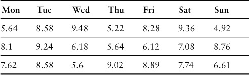
In Table 11.1, we provide three weeks of maximum load values for our application servers. The standard deviation for this sample data set is 1.49. If we take 3 times that amount, 4.48, and subtract the maximum load capacity that we have established for this server class, we then have the amount of load capacity that we can plan to use up to but not exceed. In this case, our systems administrators believe that 15 is the maximum; therefore, 15 – 4.48 = 10.5 is the maximum amount we can plan for. This is the number that we would use in the headroom equation to replace the Ideal Usage Percentage × Maximum Capacity.

Table 11.1 Load Averages

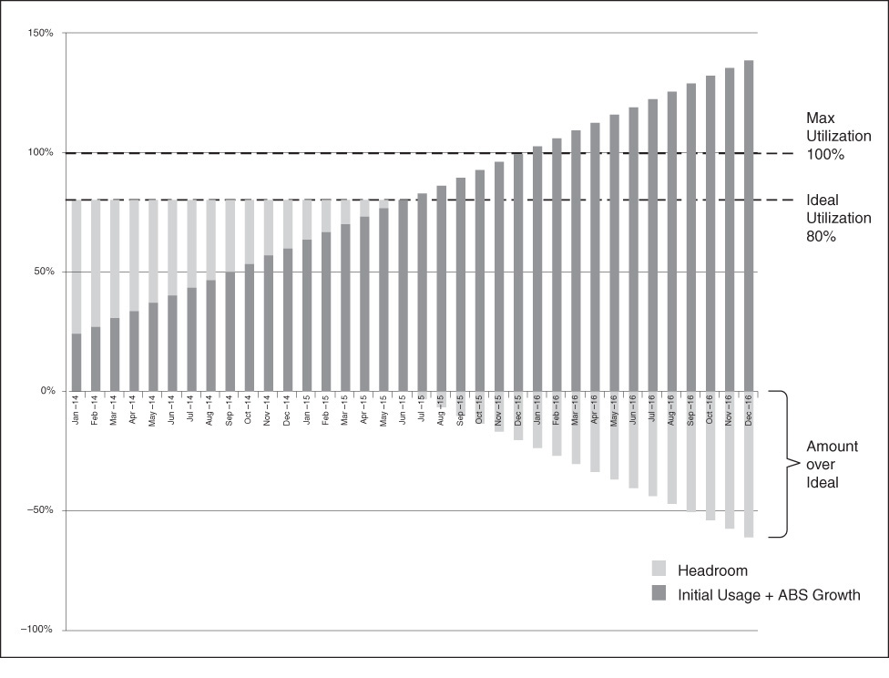
Karl was focused on defining the headroom in terms of CPU utilization for his organization. He first did all the legwork to determine business growth and ran some tests. The result was that he expected, based on the existing CPU utilization rate of 20% and the business unit expectations of growth, among other factors, that CPU utilization for the devices in question would grow at approximately 3.33% per month. This growth, as described within our equation, is an absolute growth in percentage, not compounded or relative growth to past months. Karl assigned an ideal usage of 80% to his devices and created a table like that shown in Figure 11.4. He calculated the values in this table based on three years of transactions, but we have eliminated several rows—you’ll likely get the picture of the type of information you need from the truncated version.

Figure 11.4 Headroom Calculation Table

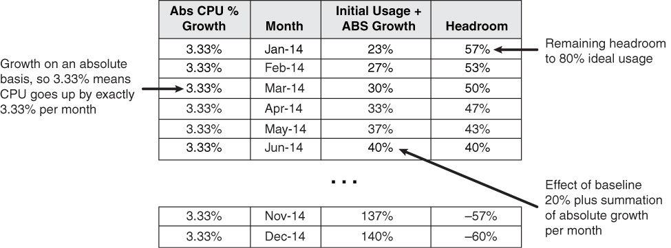
With this table in hand, it’s quite easy to plot the expected growth in transactions against the ideal utilization and determine our time to live visually. Figure 11.5 is taken from Karl Arao’s public work and modified for the purposes of this book. We can readily see in this figure that we hit our ideal limit in June 2015.

Figure 11.5 Headroom Graph

The spreadsheet method of representation also makes it easy to use compounded rates of growth. For instance, if our general manager indicated that the number of transactions is likely to grow 3% month over month (MOM), and if we knew that each transaction would have roughly the same impact on CPU utilization (or queries, or something else), we could modify the spreadsheet to compound the rate of growth. The resulting graph would have a curve in it, moving upward at increasing speeds as each month experiences significantly greater transactions than the prior month.

The headroom process consists of many steps, which are highly detail oriented, but overall it is very straightforward. The steps include identifying major components, assigning responsible parties for determining actual usage and maximum capacity for those components, and determining the intrinsic growth as well as the growth caused by business activities. Finally, you must account for seasonality and improvements in usage based on infrastructure projects, and then perform the calculations.

The last topic covered in this chapter was the ideal usage percentage for components. In general, we prefer to use a simple 50% as the amount of maximum capacity whose use should be planned. This percentage accounts for variability or mistakes in determining the maximum capacity as well as errors in the growth projects. You might be convinced to increase this percentage if your administrators or engineers can make sound and reasonable arguments for why the system is very well understood and not very variable. An alternative method of determining the maximum usage capacity is to subtract three standard deviations of actual usage from the believed maximum and then use that number as the planning maximum.

• Headroom should be calculated for each major component within the system, such as each pool of application servers, networking gear, bandwidth usage, and database servers.

• Without a sound and factually based argument for deviating from this rule of thumb, we recommend not planning on using more than 50% of the maximum capacity on any one component.