Appendix B
Thermodynamic Power Cycles: A Primer
The theoretical basis for a vast majority of the electricity generated worldwide is provided by the thermodynamic power cycles that govern the conversion of heat into mechanical work by heat engines. These power conversion cycles (PCSs) that are at the heart of fossil and nuclear power plants are also vital for electricity generation from renewable energy sources—geothermal, solar thermal, ocean thermal, and biomass. A brief overview of some of the power cycles of relevance is presented below.
B.1 Carnot Cycle
The Carnot cycle is the ideal thermodynamic process proposed by the French physicist Sadi Carnot in the early 19th century. He proposed a cyclic process consisting of two isothermal and two adiabatic steps operating between two energy reservoirs at different temperatures, as shown in Figure B.1 through the pressure–volume (P–v) and entropy–temperature (T–s) diagrams. Any substance that can undergo a cyclic process can function as the working fluid for the cycle, and the efficiency of the cycle is independent of the working fluid, as formalized by the Carnot theorem [1]:

Figure B.1 Carnot cycle.
All reversible cyclic heat engines operating between two fixed temperatures have the same efficiency.
The utility of the Carnot cycle, an ideal construct, is that it places an upper bound on the efficiency of a heat engine operating between two temperatures.
The heat input to the cycle occurs in the step 1–2, while heat rejection occurs during step 3–4. The efficiency of the engine shown in the above cycle—the Carnot efficiency—is given by equation B.1:
B.2 Brayton Cycle
The power generation in the gas turbine power plants is based on the Brayton cycle, named in honor of George Brayton, an American engineer. The cycle, which is also sometimes referred to as the Joule cycle, involves isobaric steps rather than isothermal steps, as in the Carnot cycle. The P–v and T–s diagrams for the Brayton cycle are shown in Figure B.2.
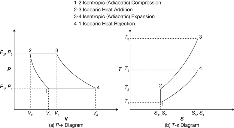
Figure B.2 Brayton cycle.
The Brayton cycle may be used for power generation in solar thermal systems.
B.3 Rankine Cycle
The Rankine cycle (as well as the Rankine absolute temperature scale) is named in honor of William John Macquorn Rankine, a Scottish engineer and physicist. It is the base cycle for vapor–liquid systems, such as the steam power plant [2]. The basic steps are the same as in the Brayton cycle; however, as the working fluid is a condensing vapor, the representation on the P–v and T–s diagrams is quite different, as shown in Figure B.3. The curve in each figure represents the boundary between phases, with the region under the dome representing a mixture of vapor and liquid. Point 3 in the figure is located in the superheated vapor region.

Figure B.3 Rankine cycle.
The Rankine cycle using steam as the working fluid may be used in solar thermal systems, as well as some geothermal systems. The temperatures in fossil thermal plants may be as high as ~550°C. The temperatures available in most geothermal systems and ocean thermal systems are generally too low to use steam as the working fluid, necessitating the use of organic working fluids, as mentioned in Chapter 5. Some of the relevant physical properties of a few working fluids for power cycles are shown in Table B.1.
Table B.1 Properties of Working Fluids Used in Power Cycles
Fluid |
Water |
Ammonia |
Propane |
R152a |
Properties |
H2O |
NH3 |
C3H8 |
CH3CHF2 |
Molecular weight |
18 |
17 |
44 |
66 |
Critical temperature, °C |
374 |
132.4 |
97 |
113.2 |
Critical pressure, MPa |
22 |
11.35 |
4.23 |
4.5 |
Normal boiling point, °C |
100 |
−33.3 |
−42.2 |
−24.7 |
Saturation pressure*, kPa |
3.2 |
1000 |
853.2 |
508 |
Enthalpy of vaporization†, kJ/mol |
40.65 |
23.4 |
24.5 |
21.8 |
B.4 Kalina Cycle
Ammonia is commonly used in OTEC Rankine cycles for power production. However, the low temperatures (25°C or less) translate to poor thermal efficiencies of ~3%. Alexander Kalina, an American scientist and engineer, devised in the late 20th century a cycle that utilizes a binary mixture, i.e., ammonia–water mixture, to minimize energy losses associated with the phase changes [3]. The T–s diagram for a simplified Kalina cycle is shown in Figure B.4 [4]. The steps occurring in the cycle are listed below:
The base ammonia solution (point 1) is heated and partially vaporized, reaching point 2, whereupon it separates into an ammonia-rich vapor (point 3) and an ammonia-poor liquid (point 5).
The ammonia-rich vapor (point 3) expands through a turbine, generating electricity and condensing partially to point 4.
The ammonia-poor liquid (point 5) is passed through a heat recovery unit and then depressurized (points 6 and 7).
The two streams (points 4 and 7) are recombined to obtain the base mixture (point 8).
The base mixture is then further subjected to heat recovery and cooling to reach point 9.
Further heating of the base solution results in reaching the initial starting point 1 of the cycle.
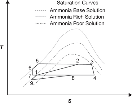
Figure B.4 Kalina cycle.
These changes can result in increasing the efficiency of power generation, possibly to as much as 5%.
The Kalina cycle was modified by Professor Haruo Uehara (known as the father of Japanese OTEC) in 1999 by incorporating two-stage turbines and improved heat recovery steps, increasing the power conversion efficiency by a further 10% [4, 5]. Further refinements of these cycles are under research and development.
B.5 Summary
As seen from equation B.1, the maximum efficiency of power conversion is limited by the difference between the temperatures of the two reservoirs—heat source and heat sink. The temperatures available in many of the primary renewable sources—geothermal and ocean thermal—are too low for the established, conventional power cycles to operate efficiently, or even make it impossible to implement them. Innovative cycles that seek to maximize the power conversion efficiency through modifying the working fluids and refining heat recovery networks are being developed all over the world. The mathematical formulations of these, as well as conventional power cycles, are available in the literature.
References
1. Goecken, N. A., and R. G. Reddy, Thermodynamics, Second Edition, Plenum Press, New York, 1996.
2. Huang, F. E., Engineering Thermodynamics: Fundamentals and Applications, Second Edition, Macmillan, New York, 1988.
3. Liu, W., et al., “A Review of Research on the Closed Thermodynamic Cycles of Ocean Thermal Energy Conversion,” Renewable and Sustainable Energy Reviews, Vol. 119, 2020, #109581, 11 pages.
4. Wang, J., et al., “Assessment of Off-Design Performance of a Kalina Cycle Driven by Low-Grade Heat Source,” Energy, Vol. 138, 2017, pp. 459–472.
5. Goto, S., et al., “Construction of Simulation Model for OTEC Plant Using Uehara Cycle,” Electrical Engineering in Japan, Vol. 176, No. 2, 2011, pp. 1–13.