Chapter 14
Sequence-to-Sequence Networks and Natural Language Translation
In Chapter 11, “Text Autocompletion with LSTM and Beam Search,” we discussed many-to-many sequence prediction problems and showed with a programming example how it can be used for autocompletion of text. Another important sequence prediction problem is to translate text from one natural language to another. In such a setting, the input sequence is a sentence in the source language, and the predicted output sequence is the corresponding sentence in the destination language. It is not necessarily the case that the sentences consist of the same number of words in the two different languages. A good English translation of the French sentence Je suis étudiant is “I am a student,” where we see that the English sentence contains one more word than its French counterpart. Another thing to note is that we want the network to consume the entire input sequence before starting to emit the output sequence, because in many cases, you need to consider the full meaning of a sentence to produce a good translation. A popular approach to handle this is to teach the network to interpret and emit START and STOP tokens as well as to ignore padding values. Both the padding value and the START and STOP tokens should be values that do not naturally appear in the text. For example, with words represented by indices that are inputs to an embedding layer, we would simply reserve specific indices for these tokens.
START tokens, STOP tokens, and padding can be used to create training examples that enable many-to-many sequences with variable lengths.
Figure 14-1 illustrates this process. The upper part of the figure shows a many-to-many network where gray represents the input, blue is the network, and green is the output. For now, ignore the ghosted (white) shapes. The network is unrolled in time from left to right. The figure shows that the desired behavior is that during the first four timesteps, we present the symbols for Je, suis, étudiant, START to the network. During the timestep that the network receives the START token, the network will output the first word (I) of the translated sentence, followed by am, a, student, and STOP during the subsequent timesteps. Let us now consider the white shapes. As previously noted, it is impossible for the network to not output a value, and similarly, the network will always get some kind of input for every timestep. This applies to the first three timesteps for the output and the last four timesteps for the input. A simple solution would be to use our padding value on both the output and the input for these timesteps. However, it turns out that a better solution is to help the network by feeding the output from the previous timestep back as input to the next timestep, just as we did in the neural language models in previous chapters. This is what is shown in the Figure 14-1.
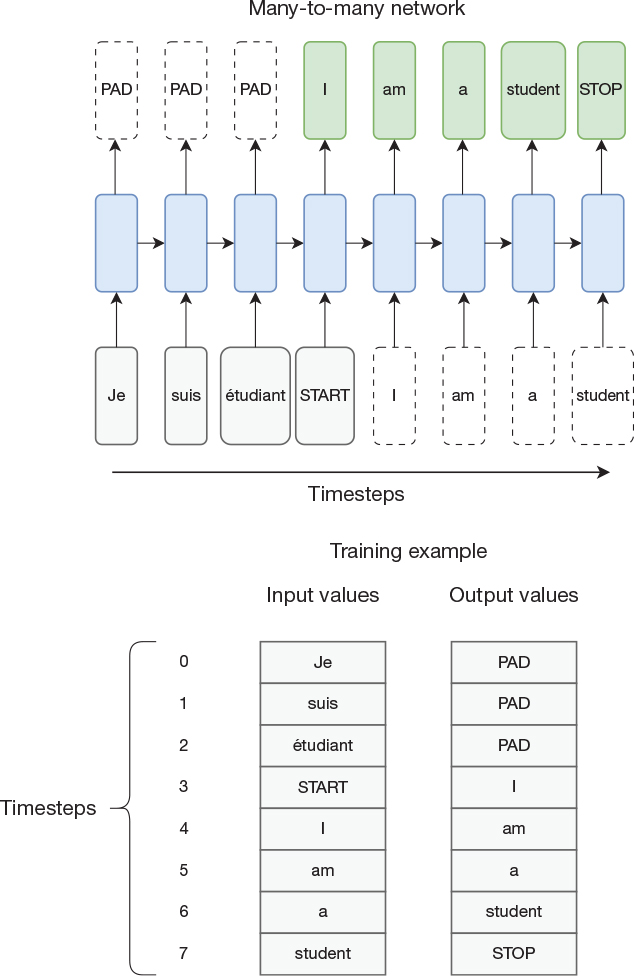
Figure 14-1 Neural machine translation is an example of a many-to-many sequence where the input and output sequences are not necessarily of the same length.
To make this abundantly clear, the lower part of the figure shows the corresponding training example without the network. That is, during training, the network will see both the source and the destination sequences on its input and be trained to predict the destination sequence on its output. Predicting the destination sequence as output might not seem that hard given that the destination sequence is also presented as input. However, they are skewed in time, so the network needs to predict the next word in the destination sequence before it has seen it. When we later use the network to produce translations, we do not have the destination sequence. We start with feeding the source sequence to the network, followed by the START token, and then start feeding back its output prediction as input to the next timestep until the network produces a STOP token. At that point, we have produced the full translated sentence.
Encoder-Decoder Model for Sequence-to-Sequence Learning
How does the model that we just described relate to the neural language models studied in previous chapters? Let us consider our translation network at the timestep when the START token is presented at its input. The only difference between this network and the neural language model networks is its initial accumulated state. In our language model, we started with 0 as internal state and presented one or more words on the input. Then the network completed the sentence. Our translation network starts with an accumulated state from seeing the source sequence, is then presented with a single START symbol, and then completes the sentence in the destination language. That is, during the second half of the translation process, the network simply acts like a neural language model in the destination language. It turns out that the internal state is all that the network needs to produce the right sentence. We can think of the internal state as a language-independent representation of the overall meaning of the sentence. Sometimes this internal state is referred to as the context or a thought vector.
Now let us consider the first half of the translation process. The goal of this phase is to consume the source sentence and build up this language-independent representation of the meaning of the sentence. Apart from being a somewhat different task than generating a sentence, it is also working with a different language/vocabulary than the second phase of the translation process. A reasonable question, then, is whether both phases should be handled by the same neural network or if it is better to have two specialized networks. The first network would be specialized in encoding the source sentence into the internal state, and the second network would be specialized in decoding the internal state into a destination sentence. Such an architecture is known as an encoder-decoder architecture, and one example is illustrated in Figure 14-2. The network is not unrolled in time. The network layers in the encoder are distinct from the network layers in the decoder. The horizontal arrow represents reading out the internal states of the recurrent layers in the encoder and initializing the internal states of the recurrent layers in the decoder. Thus, the assumption in the figure is that both networks contain the same number of hidden recurrent layers of the same size and type. In our programming example, we implement this model with two hidden recurrent layers in both networks, each consisting of 256 long short-term memory (LSTM) units.
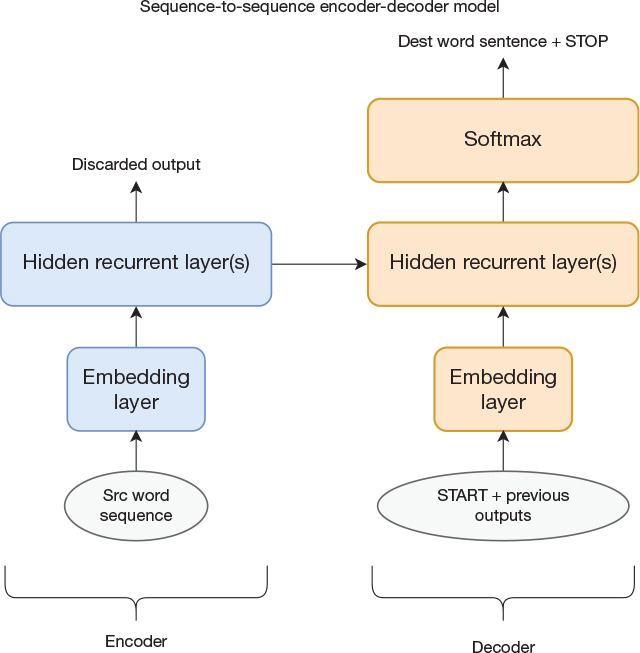
Figure 14-2 Encoder-decoder model for language translation
In an encoder-decoder architecture, the encoder creates an internal state known as context or thought vector, which is a language-independent representation of the meaning of the sentence.
Figure 14-2 shows just one example of an encoder-decoder model. Given how we evolved from a single RNN to this encoder-decoder network, it might not be that odd that the communication channel between the two networks is to transfer the internal state from one network to another. However, we should also recognize that the statement “Discarded output” is a little misleading in the figure. The internal state of an LSTM layer consists of the cell state (often denoted by c) and the recurrent layer hidden state (often denoted by h), where h is identical to the output of the layer. Similarly, if we had used a gated recurrent unit (GRU) instead of LSTM, there would not be a cell state, and the internal state of the network would be simply the recurrent layer hidden state, which again is identical to the output of the recurrent layer. Still, we chose to call it discarded output because that term is commonly found in other descriptions.
One can envision other ways of connecting the encoder and the decoder. For example, we could feed the state/output as a regular input to the decoder just during the first timestep, or we could give the decoder network access to it during each timestep. Or, in the case of an encoder with multiple layers, we could choose to just present the state/output from the topmost layer as inputs to the bottommost decoder layer. It is also worth noting that encoder-decoder models are not limited to working with sequences. We can construct other combinations, such as cases where only one of the encoder or decoder, or neither of them, has recurrent layers. We discuss more details about this in the next couple of chapters, but at this point, we move on to implementing our neural machine translator (NMT) in Keras.
Encoder-decoder architectures can be built in many different ways. Different network types can be used for the encoder and decoder, and the connection between the two can also be done in multiple ways.
Introduction to the Keras Functional API
It is not obvious how to implement the described architecture using the constructs that we have used in the Keras API so far. To implement this architecture, we need to use the Keras Functional API, which is specifically created to enable creation of complex models. There is a key difference compared to using the sequential models that we have used so far. Instead of just declaring a layer and adding to the model and letting Keras automatically connect the layers in a sequential manner, we now need to explicitly describe how layers are connected to each other. This process is more complex and error prone than letting Keras do it for us, but the benefit is the increased flexibility that enables us to describe a more complex model.
Keras Functional API is more flexible than the Sequential API and can therefore be used to build more complex network architectures.
We use the example models in Figure 14-3 to illustrate how to use the Keras Functional API. The model to the left is a simple sequential model that could easily have been implemented with the Sequential API, but the model to the right has an input that bypasses the first layer and therefore needs to use the Functional API.
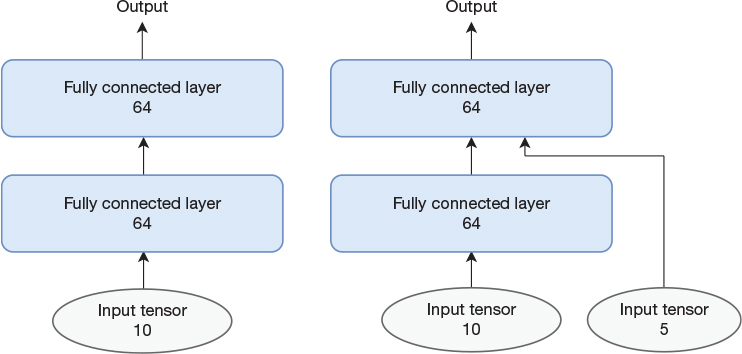
Figure 14-3 Two simple models. The left one is straightforward to implement with the Sequential API, but the right one requires the Functional API.
The implementation of the left model is shown in Code Snippet 14-1. We start by declaring an Input object. This is different from the Sequential API, where the input layer was implicitly created when the first layer was created. We then declare the two fully connected layers in the model. Once this is done, it is time to connect the layers by using the assigned variable name as a function and passing it its inputs as an argument. The function returns an object representing the outputs of the layer, which can then be used as input argument when connecting the next layer.
Code Snippet 14-1 Example How to Implement a Simple Sequential Model Using the Functional API
from tensorflow.keras.layers import Input, Dense
from tensorflow.keras.models import Model

# Declare inputs.
inputs = Input(shape=(10,))

# Declare layers.
layer1 = Dense(64, activation='relu')
layer2 = Dense(64, activation='relu')

# Connect inputs and layers.
layer1_outputs = layer1(inputs)
layer2_outputs = layer2(layer1_outputs)

# Create model.
model = Model(inputs=inputs, outputs=layer2_outputs)
model.summary()
Now that we have declared and connected layers to each other, we are ready to create the model. This is done by simply calling the Model() constructor and providing arguments informing the model what its inputs and outputs should be.
Creating the more complex model with a bypass path from the input to the second layer is shown in Code Snippet 14-2. There are just a few minor changes compared to the previous example. First, we declare two sets of inputs. One is the input to the first layer, and the other is the bypass input that will go straight to the second layer. Next, we declare a Concatenate layer, which is used to concatenate the outputs from the first layer with the bypass input to form a single variable that can be provided as input to the second layer. Finally, when declaring the model, we need to tell it that its inputs now consist of a list of two inputs.
Code Snippet 14-2 Keras Implementation of a Network with a Bypass Path
from tensorflow.keras.layers import Input, Dense
from tensorflow.keras.models import Model
from tensorflow.keras.layers import Concatenate

# Declare inputs.
inputs = Input(shape=(10,))
bypass_inputs = Input(shape=(5,))

# Declare layers.
layer1 = Dense(64, activation='relu')
concat_layer = Concatenate()
layer2 = Dense(64, activation='relu')

# Connect inputs and layers.
layer1_outputs = layer1(inputs)
layer2_inputs = concat_layer([layer1_outputs, bypass_inputs])
layer2_outputs = layer2(layer2_inputs)

# Create model.
model = Model(inputs=[inputs, bypass_inputs],
              outputs=layer2_outputs)
model.summary()
After this brief introduction to the Keras Functional API, we are ready to move on to implementing our neural machine translation network.
Programming Example: Neural Machine Translation
As usual, we begin by importing modules that we need for the program. This is shown in Code Snippet 14-3.
Code Snippet 14-3 Import Statements
import numpy as np
import random
from tensorflow.keras.layers import Input
from tensorflow.keras.layers import Embedding
from tensorflow.keras.layers import LSTM
from tensorflow.keras.layers import Dense
from tensorflow.keras.models import Model
from tensorflow.keras.optimizers import RMSprop
from tensorflow.keras.preprocessing.text import Tokenizer
from tensorflow.keras.preprocessing.text
    import text_to_word_sequence
from tensorflow.keras.preprocessing.sequence
    import pad_sequences
import tensorflow as tf
import logging
tf.get_logger().setLevel(logging.ERROR)
Next, we define some constants in Code Snippet 14-4. We specify a vocabulary size of 10,000 symbols, out of which four indices are reserved for padding, out-of-vocabulary words (denoted as UNK), START tokens, and STOP tokens. Our training corpus is large, so we set the parameter READ_LINES to the number of lines in the input file we want to use in our example (60,000). Our layers consist of 256 units (LAYER_SIZE), and the embedding layers output 128 dimensions (EMBEDDING_WIDTH). We use 20% (TEST_PERCENT) of the dataset as test set and further select 20 sentences (SAMPLE_SIZE) to inspect in detail during training. We limit the length of the source and destination sentences to, at most, 60 words (MAX_LENGTH). Finally, we provide the path to the data file, where each line is expected to contain two versions of the same sentence (one in each language) separated by a tab character.
Code Snippet 14-4 Definition of Constants
# Constants
EPOCHS = 20
BATCH_SIZE = 128
MAX_WORDS = 10000
READ_LINES = 60000
LAYER_SIZE = 256
EMBEDDING_WIDTH = 128
TEST_PERCENT = 0.2
SAMPLE_SIZE = 20
OOV_WORD = 'UNK'
PAD_INDEX = 0
OOV_INDEX = 1
START_INDEX = MAX_WORDS - 2
STOP_INDEX = MAX_WORDS - 1
MAX_LENGTH = 60
SRC_DEST_FILE_NAME = '../data/fra.txt'
Code Snippet 14-5 shows the function used to read the input data file and do some initial processing. Each line is split into two strings, where the first contains the sentence in the destination language and the second contains the sentence in the source language. We use the function text_to_word_sequence() to clean the data somewhat (make everything lowercase and remove punctuation) and split each sentence into a list of individual words. If the list (sentence) is longer than the maximum allowed length, then it is truncated.
Code Snippet 14-5 Function to Read Input File and Create Source and Destination Word Sequences
# Function to read file.
def read_file_combined(file_name, max_len):
    file = open(file_name, 'r', encoding='utf-8')
    src_word_sequences = []
    dest_word_sequences = []
    for i, line in enumerate(file):
        if i == READ_LINES:
            break
        pair = line.split('	')
        word_sequence = text_to_word_sequence(pair[1])
        src_word_sequence = word_sequence[0:max_len]
        src_word_sequences.append(src_word_sequence)
        word_sequence = text_to_word_sequence(pair[0])
        dest_word_sequence = word_sequence[0:max_len]
        dest_word_sequences.append(dest_word_sequence)
    file.close()
    return src_word_sequences, dest_word_sequences
Code Snippet 14-6 shows functions used to turn sequences of words into sequences of tokens, and vice versa. We call tokenize() a single time for each language, so the argument sequences is a list of lists where each of the inner lists represents a sentence. The Tokenizer class assigns indices to the most common words and returns either these indices or the reserved OOV_INDEX for less common words that did not make it into the vocabulary. We tell the Tokenizer to use a vocabulary of 9998 (MAX_WORDS-2)—that is, use only indices 0 to 9997, so that we can use indices 9998 and 9999 as our START and STOP tokens (the Tokenizer does not support the notion of START and STOP tokens but does reserve index 0 to use as a padding token and index 1 for out-of-vocabulary words). Our tokenize() function returns both the tokenized sequence and the Tokenizer object itself. This object will be needed anytime we want to convert tokens back into words.
Code Snippet 14-6 Functions to Turn Word Sequences into Tokens, and Vice Versa
# Functions to tokenize and un-tokenize sequences.
def tokenize(sequences):
    # "MAX_WORDS-2" used to reserve two indices
    # for START and STOP.
    tokenizer = Tokenizer(num_words=MAX_WORDS-2,
                          oov_token=OOV_WORD)
    tokenizer.fit_on_texts(sequences)
    token_sequences = tokenizer.texts_to_sequences(sequences)
    return tokenizer, token_sequences

def tokens_to_words(tokenizer, seq):
    word_seq = []
    for index in seq:
        if index == PAD_INDEX:
            word_seq.append('PAD')
        elif index == OOV_INDEX:
            word_seq.append(OOV_WORD)
        elif index == START_INDEX:
            word_seq.append('START')
        elif index == STOP_INDEX:
            word_seq.append('STOP')
        else:
            word_seq.append(tokenizer.sequences_to_texts(
                [[index]])[0])
    print(word_seq)
The function tokens_to_words() requires a Tokenizer and a list of indices. We simply check for the reserved indices: If we find a match, we replace them with hardcoded strings, and if we find no match, we let the Tokenizer convert the index to the corresponding word string. The Tokenizer expects a list of lists of indices and returns a list of strings, which is why we need to call it with [[index]] and then select the 0th element to arrive at a string.
Now, given that we have these helper functions, it is trivial to read the input data file and convert into tokenized sequences. This is done in Code Snippet 14-7.
Code Snippet 14-7 Read and Tokenize the Input File
# Read file and tokenize.
src_seq, dest_seq = read_file_combined(SRC_DEST_FILE_NAME,
                                       MAX_LENGTH)
src_tokenizer, src_token_seq = tokenize(src_seq)
dest_tokenizer, dest_token_seq = tokenize(dest_seq)
It is now time to arrange the data into tensors that can be used for training and testing. In Figure 14-1, we indicated that we need to pad the start of the output sequence with as many PAD symbols as there are words in the input sequence, but that was when we envisioned a single neural network. Now that we have broken up the network into an encoder and a decoder, this is no longer necessary because we will simply not input anything to the decoder until we have run the full input through the encoder. Following is a more accurate example of what we need as input and output for a single training example, where src_input is the input to the encoder network, dest_input is the input to the decoder network, and dest_target is the desired output from the decoder network:
src_input = [PAD, PAD, PAD, id(“je”), id(“suis”),
id(“étudiant”)]

dest_input = [START, id(“i”), id(“am”), id(“a”),
id(“student”), STOP, PAD, PAD]

dest_target = [one_hot_id(“i”), one_hot_id(“am”), one_hot_
id(“a”), one_hot_id(“student”), one_hot_id(STOP), one_hot_
id(PAD), one_hot_id(PAD), one_hot_id(PAD)]
In the example, id(string) refers to the tokenized index of the string, and one_hot_id is the one-hot encoded version of the index. We have assumed that the longest source sentence is six words, so we padded src_input to be of that length. Similarly, we have assumed that the longest destination sentence is eight words including START and STOP tokens, so we padded both dest_input and dest_target to be of that length. Note how the symbols in dest_input are offset by one location compared to the symbols in dest_target because when we later do inference, the inputs into the decoder network will be coming from the output of the network for the previous timestep. Although this example has shown the training example as being lists, in reality, they will be rows in NumPy arrays, where each array contains multiple training examples.
The padding is done to ensure that we can use mini-batches for training. That is, all source sentences need to be the same length, and all destination sentences need to be the same length. We pad the source input at the beginning (known as prepadding) and the destination at the end (known as postpadding), which is nonobvious. We previously stated that when using padding, the model can learn to ignore the padded values, but there is also a mechanism in Keras to mask out padded values. Based on these two statements, it seems like it should not matter whether the padding is at the beginning or end. However, as always, things are not as simple as they might appear. If we start with the assumption of the model learning to ignore values, it will not perfectly learn this. The ease with which it learns to ignore padding values might depend on how the data is arranged. It is not hard to imagine that inputting a considerable number of zeros at the end of a sequence will dilute the input and affect the internal state of the network. From that perspective, it makes sense to pad the input values with zeros in the beginning of the sequence instead. Similarly, in a sequence-to-sequence network, if the encoder has created an internal state that is transferred to the decoder, diluting this state by presenting a number of zeros before the START token also seems like it could be bad.
This reasoning supports the chosen padding (prepadding of the source input and postpadding of the destination input) in a case where the network needs to learn to ignore the padded values. However, given that we will use the mask_zero=True parameter for our embedding layers, it should not matter what type of padding we use. It turns out that the behavior of mask_zero is not what we had expected when using it for our custom encoder-decoder network. We observed that the network learned poorly when we used postpadding for the source input. We do not know the exact reason for this but suspect that there is some interaction where the masked input values to the encoder somehow causes the decoder to ignore the beginning of the output sequences.1
1. This is just a theory, and the behavior could be something else. Further, it is unclear to us whether it is due to a bug or an expected but undocumented behavior. Regardless, when using the suggested padding, we do not see the problem.
Padding can be done in the beginning or end of the sequence. This is known as prepadding and postpadding.
Code Snippet 14-8 shows a compact way of creating the three arrays that we need. The first two lines create two new lists, each containing the destination sequences but the first (dest_target_token_seq) also augmented with STOP_INDEX after each sequence and the second (dest_input_token_seq) augmented with both START_INDEX and STOP_INDEX. It is easy to miss that dest_input_token_seq has a STOP_INDEX, but that falls out naturally because it is created from the dest_target_token_seq for which a STOP_INDEX was just added to each sentence.
Code Snippet 14-8 Compact Version of Code to Convert the Tokenized Sequences into NumPy Arrays
# Prepare training data.
dest_target_token_seq = [x + [STOP_INDEX] for x in dest_token_seq]
dest_input_token_seq = [[START_INDEX] + x for x in
                        dest_target_token_seq]
src_input_data = pad_sequences(src_token_seq)
dest_input_data = pad_sequences(dest_input_token_seq,
                                padding='post')
dest_target_data = pad_sequences(
    dest_target_token_seq, padding='post', maxlen
    = len(dest_input_data[0]))
Next, we call pad_sequences() on both the original src_input_data list (of lists) and on these two new destination lists. The pad_sequences() function pads the sequences with the PAD value and then returns a NumPy array. The default behavior of pad_sequences is to do prepadding, and we do that for the source sequence but explicitly ask for postpadding for the destination sequences. You might wonder why there is no call to to_categorical() in the statement that creates the target (output) data. We are used to wanting to have the ground truth one-hot encoded for textual data. Not doing so is an optimization to avoid wasting too much memory. With a vocabulary of 10,000 words, and 60,000 training examples, where each training example is a sentence, the memory footprint of the one-hot encoded data starts becoming a problem. Therefore, instead of one-hot encoding all data up front, there is a way to let Keras deal with that in the loss function itself.
Before we build our model, Code Snippet 14-9 demonstrates how we can manually split our dataset into a training dataset and a test dataset. In previous examples, we either relied on datasets that are already split this way or we used functionality inside of Keras when calling the fit() function. However, in this case, we want some more control ourselves because we will want to inspect a few select members of the test set in detail. We split the dataset by first creating a list test_indices, which contains a 20% (TEST_PERCENT) subset of all the numbers from 0 to N–1, where N is the size of our original dataset. We then create a list train_indices, which contains the remaining 80%. We can now use these lists to select a number of rows in the matrices representing the dataset and create two new collections of matrices, one to be used as training set and one to be used as test set. Finally, we create a third collection of matrices, which only contains 20 (SAMPLE_SIZE) random examples from the test dataset. We will use them to inspect the resulting translations in detail, but since that is a manual process, we limit ourselves to a small number of sentences.
Code Snippet 14-9 Manually Splitting the Dataset into a Training Set and a Test Set
# Split into training and test set.
rows = len(src_input_data[:,0])
all_indices = list(range(rows))
test_rows = int(rows * TEST_PERCENT)
test_indices = random.sample(all_indices, test_rows)
train_indices = [x for x in all_indices if x not in test_indices]

train_src_input_data = src_input_data[train_indices]
train_dest_input_data = dest_input_data[train_indices]
train_dest_target_data = dest_target_data[train_indices]

test_src_input_data = src_input_data[test_indices]
test_dest_input_data = dest_input_data[test_indices]
test_dest_target_data = dest_target_data[test_indices]

# Create a sample of the test set that we will inspect in detail.
test_indices = list(range(test_rows))
sample_indices = random.sample(test_indices, SAMPLE_SIZE)
sample_input_data = test_src_input_data[sample_indices]
sample_target_data = test_dest_target_data[sample_indices]
As usual, we have now spent a whole lot of code just preparing the data, but we are finally ready to build our model. This time, building the model will be more exciting than in the past because we are now building a less trivial model and will make use of the Keras Functional API.
Before going over the code, we revisit the architecture of the model that we intend to build. The network consists of an encoder part and a decoder part. We define these as two separate models, which we later tie together. The two models are illustrated in Figure 14-4. The upper part of the figure shows the encoder, which consists of an embedding layer and two LSTM layers. The lower part of the figure shows the decoder, which consists of an embedding layer, two LSTM layers, and a fully connected softmax layer. The names in the figure correspond to the variable names that we use in our implementation.
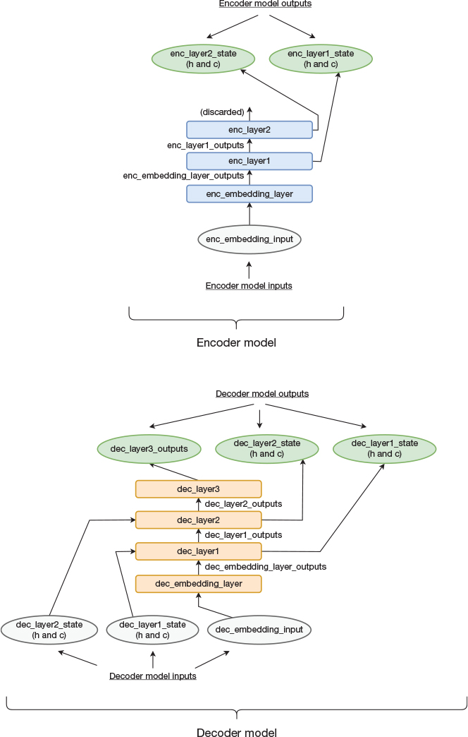
Figure 14-4 Topology of the encoder and decoder models
Apart from the layer names, the figure also contains names of the outputs of all layers, which will be used in the code when connecting layers. Four noteworthy outputs (illustrated as two sets of outputs) are the state outputs from the two encoder LSTM layers. These are used as inputs into the decoder LSTM layers to communicate the accumulated state from the encoder to the decoder.
Code Snippet 14-10 contains the implementation of the encoder model. It should be straightforward to map the code to Figure 14-4, but there are a few things worth pointing out. Because we are now interested in accessing the internal state of the LSTM layers, we need to provide the argument return_state=True. This argument instructs the LSTM object to return not only a variable representing the layer’s output but also variables representing the c and h states. Further, as previously described, for a recurrent layer that feeds another recurrent layer, we need to provide the argument return_sequences=True so that the subsequent layer sees the outputs of each timestep. This is also true for the final recurrent layer if we want the network to produce an output during each timestep. For our encoder, we are only interested in the final state, so we do not set return_sequences to True for enc_layer2.
Code Snippet 14-10 Implementation of Encoder Model
# Build encoder model.
# Input is input sequence in source language.
enc_embedding_input = Input(shape=(None, ))
# Create the encoder layers.
enc_embedding_layer = Embedding(
    output_dim=EMBEDDING_WIDTH, input_dim
    = MAX_WORDS, mask_zero=True)
enc_layer1 = LSTM(LAYER_SIZE, return_state=True,
                  return_sequences=True)
enc_layer2 = LSTM(LAYER_SIZE, return_state=True)
# Connect the encoder layers.
# We don't use the last layer output, only the state.
enc_embedding_layer_outputs =
    enc_embedding_layer(enc_embedding_input)
enc_layer1_outputs, enc_layer1_state_h, enc_layer1_state_c =
    enc_layer1(enc_embedding_layer_outputs)
_, enc_layer2_state_h, enc_layer2_state_c =
    enc_layer2(enc_layer1_outputs)

# Build the model.
enc_model = Model(enc_embedding_input,
                  [enc_layer1_state_h, enc_layer1_state_c,
                   enc_layer2_state_h, enc_layer2_state_c])
enc_model.summary()
Once all layers are connected, we create the actual model by calling the Model() constructor and providing arguments to specify what inputs and outputs will be external to the model. The model takes the source sentence as input and produces the internal states of the two LSTM layers as outputs. Each LSTM layer has both an h state and c state, so in total, the model will output four state variables as output. Each state variable is in itself a tensor consisting of multiple values.
Code Snippet 14-11 shows the implementation of the decoder model. In addition to the sentence in the destination language, it takes the output state from the encoder model as inputs. We initialize the decoder LSTM layers (using the argument initial_state) with this state at the first timestep.
Code Snippet 14-11 Implementation of Decoder Model
# Build decoder model.
# Input to the network is input sequence in destination
# language and intermediate state.
dec_layer1_state_input_h = Input(shape=(LAYER_SIZE,))
dec_layer1_state_input_c = Input(shape=(LAYER_SIZE,))
dec_layer2_state_input_h = Input(shape=(LAYER_SIZE,))
dec_layer2_state_input_c = Input(shape=(LAYER_SIZE,))
dec_embedding_input = Input(shape=(None, ))

# Create the decoder layers.
dec_embedding_layer = Embedding(output_dim=EMBEDDING_WIDTH,
                                input_dim=MAX_WORDS,
                                mask_zero=True)
dec_layer1 = LSTM(LAYER_SIZE, return_state = True,
                  return_sequences=True)
dec_layer2 = LSTM(LAYER_SIZE, return_state = True,
                  return_sequences=True)
dec_layer3 = Dense(MAX_WORDS, activation='softmax')

# Connect the decoder layers.
dec_embedding_layer_outputs = dec_embedding_layer(
    dec_embedding_input)
dec_layer1_outputs, dec_layer1_state_h, dec_layer1_state_c =
    dec_layer1(dec_embedding_layer_outputs,
    initial_state=[dec_layer1_state_input_h,
                   dec_layer1_state_input_c])
dec_layer2_outputs, dec_layer2_state_h, dec_layer2_state_c =
    dec_layer2(dec_layer1_outputs,
    initial_state=[dec_layer2_state_input_h,
                   dec_layer2_state_input_c])
dec_layer3_outputs = dec_layer3(dec_layer2_outputs)

# Build the model.
dec_model = Model([dec_embedding_input,
                   dec_layer1_state_input_h,
                   dec_layer1_state_input_c,
                   dec_layer2_state_input_h,
                   dec_layer2_state_input_c],
                  [dec_layer3_outputs, dec_layer1_state_h,
                   dec_layer1_state_c, dec_layer2_state_h,
                   dec_layer2_state_c])
dec_model.summary()
For the decoder, we do want the top LSTM layer to produce an output for each timestep (the decoder should create a full sentence and not just a final state), so we set return_sequences=True for both LSTM layers.
We create the model by calling the Model() constructor. The inputs consist of the destination sentence (time shifted by one timestep) and initial state for the LSTM layers. As we soon will see, when using the model for inference, we need to explicitly manage the internal state for the decoder. Therefore, we declare the states as outputs of the model in addition to the softmax output.
We are now ready to connect the two models to build a full encoder-decoder network corresponding to what is shown in Figure 14-5. The corresponding TensorFlow implementation is shown in Code Snippet 14-12.
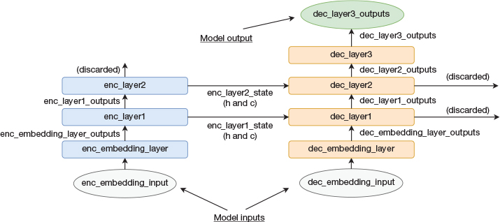
Figure 14-5 Architecture of full encoder-decoder model
Code Snippet 14-12 Code to Define, Build, and Compile the Model Used for Training
# Build and compile full training model.
# We do not use the state output when training.
train_enc_embedding_input = Input(shape=(None, ))
train_dec_embedding_input = Input(shape=(None, ))
intermediate_state = enc_model(train_enc_embedding_input)
train_dec_output, _, _, _, _ = dec_model(
    [train_dec_embedding_input] +
    intermediate_state)
training_model = Model([train_enc_embedding_input,
                        train_dec_embedding_input],
                        train_dec_output)
optimizer = RMSprop(lr=0.01)
training_model.compile(loss='sparse_categorical_crossentropy',
                       optimizer=optimizer, metrics =['accuracy'])
training_model.summary()
One thing that looks odd is that, as we described previously, we provide the argument return_state=True when creating the decoder LSTM layers, but then when we create this model, we discard the state outputs. It seems reasonable to not have set the return_state=True argument to begin with. The reason will be apparent when we describe how to use the encoder and decoder models for inference.
We decided to use RMSProp as optimizer because some experiments indicate that it performs better than Adam for this specific model. We use sparse_categorical_crossentropy instead of the normal categorical_crossentropy as loss function. This is the loss function to use in Keras if the categorical output data is not already one-hot encoded. As described earlier, we avoided one-hot encoding the data up front to reduce the memory footprint of the application.
Although we just connected the encoder and decoder model to form a joint model, they can both still be used in isolation. Note that the encoder and decoder models used by the joint model are the same instances as the individual models. That is, if we train the joint model, it will update the weights of the first two models. This is useful because, when we do inference, we want an encoder model that is decoupled from the decoder model.
During inference, we first run the source sentence through the encoder model to create the internal state. This state is then provided as initial state to the decoder model during the first timestep. At this timestep, we also feed the START token to the embedding layer of the model. This results in the model producing the first word in the translated sentence as its output. It also produces outputs representing the internal state of the two LSTM layers. In the next timestep, we feed the model with the predicted output as well as the internal state from the previous timestep (we explicitly manage the internal state) in an autoregressive manner.
Instead of explicitly managing the state, we could have declared the layers as stateful=True, as we did in our text autocompletion example, but that would complicate the training process. We cannot have stateful=True during training if we do not want multiple subsequent training examples to affect each other.
Finally, the reason that we do not need to explicitly manage state during training is that we fed the entire sentence at once to the model, in which case TensorFlow automatically feeds the state from the last timestep back to be used as the current state for the next timestep.
This whole discussion may seem unclear until you get more familiar with Keras, but the short of it is that there are many ways of doing the same thing and each method has its own benefits and drawbacks.
When declaring a recurrent layer in Keras, there are three arguments: return_state, return_sequences, and stateful. At first, it can be tricky to tell them apart because of their similar names. If you want to build your own complicated networks, it is well worth spending some time to fully understand what they do and how they interact with each other.
We are now ready to train and test the model, which is shown in Code Snippet 14-13. We take a slightly different approach than in previous examples. In previous examples, we instructed fit() to train for multiple epochs, and then we studied the results and ended our program. In this example, we create our own training loop where we instruct fit() to train for only a single epoch at a time. We then use our model to create some predictions before going back and training for another epoch. This approach enables some detailed evaluation of just a small set of samples after each epoch. We could have done this by providing a callback function as an argument to the fit function, but we figured that it was unnecessary to introduce yet another Keras construct at this point.
Code Snippet 14-13 Training and Testing the Model
# Train and test repeatedly.
for i in range(EPOCHS):
    print('step: ' , i)
    # Train model for one epoch.
    history = training_model.fit(
        [train_src_input_data, train_dest_input_data],
        train_dest_target_data, validation_data=(
            [test_src_input_data, test_dest_input_data],
            test_dest_target_data), batch_size=BATCH_SIZE,
        epochs=1)

    # Loop through samples to see result
    for (test_input, test_target) in zip(sample_input_data,
                                         sample_target_data):
        # Run a single sentence through encoder model.
        x = np.reshape(test_input, (1, -1))
        last_states = enc_model.predict(
            x, verbose=0)
        # Provide resulting state and START_INDEX as input
        # to decoder model.
        prev_word_index = START_INDEX
        produced_string = ''
        pred_seq = []
        for j in range(MAX_LENGTH):
            x = np.reshape(np.array(prev_word_index), (1, 1))
            # Predict next word and capture internal state.
            preds, dec_layer1_state_h, dec_layer1_state_c,
                dec_layer2_state_h, dec_layer2_state_c =
                    dec_model.predict(
                        [x] + last_states, verbose=0)
            last_states = [dec_layer1_state_h,
                           dec_layer1_state_c,
                           dec_layer2_state_h,
                           dec_layer2_state_c]
            # Find the most probable word.
            prev_word_index = np.asarray(preds[0][0]).argmax()
            pred_seq.append(prev_word_index)
            if prev_word_index == STOP_INDEX:
                break
        tokens_to_words(src_tokenizer, test_input)
        tokens_to_words(dest_tokenizer, test_target)
        tokens_to_words(dest_tokenizer, pred_seq)
        print('

')
Keras callback functions is a good topic for further reading if you want to customize the behavior of the training process (keras.io).
Most of the code sequence is the loop used to create translations for the smaller set of samples that we created from the test dataset. This piece of code consists of a loop that iterates over all the examples in sample_input_data. We provide the source sentence to the encoder model to create the resulting internal state and store to the variable last_states. We also initialize the variable prev_word_index with the index corresponding to the START symbol. We then enter the innermost loop and predict a single word using the decoder model. We also read out the internal state. This data is then used as input to the decoder model in the next iteration, and we iterate until the model produces a STOP token or until a given number of words have been produced. Finally, we convert the produced tokenized sequences into the corresponding word sequences and print them out.
Experimental Results
Training the network for 20 epochs resulted in high accuracy metrics for both training and test data. Accuracy is not necessarily the most meaningful metric to use when working on machine translation, but it still gives us some indication that our translation network works. More interesting is to inspect the resulting translations for our sample set.
The first example is shown here:
['PAD', 'PAD', 'PAD', 'PAD', 'PAD', 'PAD', 'PAD', 'PAD', 'PAD',
'PAD', "j'ai", 'travaillé', 'ce', 'matin']
['i', 'worked', 'this', 'morning', 'STOP', 'PAD', 'PAD', 'PAD',
'PAD', 'PAD']
['i', 'worked', 'this', 'morning', 'STOP']
The first line shows the input sentence in French. The second line shows the corresponding training target, and the third line shows the prediction from our trained model. That is, for this example, the model predicted the translation exactly right!
Additional examples are shown in Table 14-1, where we have stripped out the padding and STOP tokens as well as removed characters associated with printing out the Python lists. When looking at the first two examples, it should be clear why we said that accuracy is not necessarily a good metric. The prediction is not identical to the training target, so the accuracy would be low. Still, it is hard to argue that the translations are wrong, given that the predictions express the same meaning as the targets. To address this, a metric known as BiLingual Evaluation Understudy (BLEU) score is used within the machine translation community (Papineni et al., 2002). We do not use or discuss that metric further, but it is certainly something to learn about if you want to dive deeper into machine translation. For now, we just recognize that there can be multiple correct translations to a single sentence.
Table 14-1 Examples of Translations Produced by the Model
SOURCE |
TARGET |
PREDICTION |
|---|---|---|
je déteste manger seule |
i hate eating alone |
i hate to eat alone |
je n’ai pas le choix |
i don’t have a choice |
i have no choice |
je pense que tu devrais le faire |
i think you should do it |
i think you should do it |
tu habites où |
where do you live |
where do you live |
nous partons maintenant |
we’re leaving now |
we’re leaving now |
j’ai pensé que nous pouvions le faire |
i thought we could do it |
i thought we could do it |
je ne fais pas beaucoup tout ça |
i don’t do all that much |
i’m not busy at all |
il a été élu roi du bal de fin d’année |
he was voted prom king |
he used to negotiate and look like golfer |
BLEU score can be used to judge how well a machine translation system works (Papineni et al., 2002). Learning the details of how it is computed makes sense if you want to dive deeper into machine translation.
Looking at the third through sixth rows, it almost seems too good to be true. The translations are identical to the expected translations. Is it possible for the model to be that good? Inspecting the training data gives us a clue about what is going on. It turns out that the dataset contains many minor variations of a single sentence in the source language, and all these sentences are translated to the same sentence in the destination language. Thus, the model is trained on a specific source/target sentence pair and is later presented with a slightly different source sentence. It is not all that unexpected that the model then predicts exactly the same target sentence that it was trained on, so we might view this as cheating. On the other hand, we do want to train the model to recognize similarities and be able to generalize, so it is not completely obvious that we should strip out these training examples. Still, we did some experiments where we removed any training example that had a duplicate in either the source or the destination language, and the model still performed well. Thus, the model clearly does not fully rely on cheating.
One example of where the model does work without cheating is the second to last example. The test example has the sentence “I don’t do all that much” as target. The model predicts the fairly different sentence “I’m not busy at all,” which arguably still conveys a similar message. Interestingly, when searching through the whole dataset, the phrase “busy at all” does not show up a single time, so the model constructed that translation from smaller pieces. On the other hand, the model also produces some translations that are just wrong. For the last example in the table, the target was “he was voted prom king” but the model came up with “he used to negotiate and look like golfer.”
Properties of the Intermediate Representation
We previously showed that the word embeddings learned in a neural language model capture some syntactic and semantic structure of the language it models. Sutskever, Vinyals, and Le (2014) made a similar observation when analyzing the intermediate representation produced by the encoder in a sequence-to-sequence model. They used principal component analysis (PCA) to reduce this representation to two dimensions to be able to visualize the vectors. For the purpose of this discussion, the only thing you need to know about PCA is that the resulting lower dimensional vectors still maintain some properties of the original vectors. In particular, if two vectors are similar to each other before reducing the dimensionality, then these two vectors will still be similar to each other in the new lower dimensional space.2
2. PCA can also be used to reduce the dimensionality of word embeddings and plot them in 2D space to be able to visualize their similarity.
PCA can be used to reduce the number of dimensions of a set of vectors. It is a good technique to know if working with vector representations in many-dimensional spaces.
Figure 14-6 shows a chart that visualizes the intermediate representation of six phrases. The six phrases are grouped into two groups of three phrases each, where the three phrases within a single group express approximately the same meaning but with some grammatical variations (e.g., passive voice and word order). However, phrases in different groups express different meanings. Interestingly, as can be seen in the chart, the intermediate representation chosen by the model is such that the three phrases with similar meaning also have similar encodings, and they cluster together.
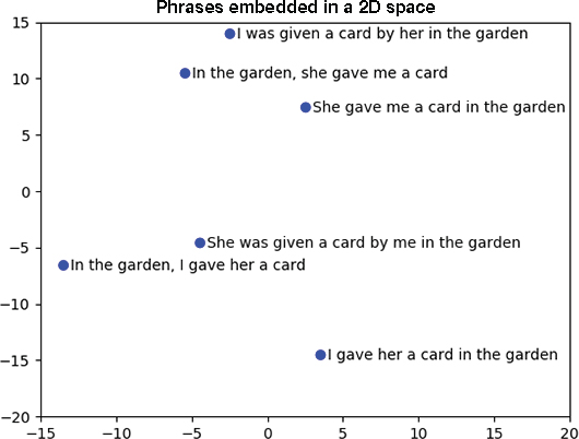
Figure 14-6 2D representation of intermediate representation of six sentences. (Source: Adapted from Sutskever, I., Vinyals, O., and Le, Q. (2014), “Sequence to Sequence Learning with Neural Networks,” in Proceedings of the 27th International Conference on Neural Information Processing [NIPS’14], MIT Press, 3104–3112.)
We can view this intermediate representation as a sentence embedding or phrase embedding, where similar phrases will be embedded close to each other in vector space. Hence, we can use this encoding to analyze the semantics of phrases. Looking at the example, it seems likely that this methodology will be more powerful than the previously discussed bag-of-word approach. As opposed to the bag-of-word approach, the sequence-to-sequence model does take word order into account.
Concluding Remarks on Language Translation
Although this programming example was longer and more complicated than most examples we have shown so far, from a software development point of view, it is a simple implementation. It is a basic encoder-decoder architecture without any bells and whistles, and it consists of fewer than 300 lines of code. If you are interested in experimenting with this model to improve translation quality, a starting point is to tweak the network by increasing the number of units in the layers or increasing the number of layers. You can also experiment with using bidirectional layers instead of unidirectional layers. One problem that has been observed is that sequence-to-sequence networks of this type find it challenging to deal with long sentences. A simple trick that mitigates this problem is to reverse the input sentence. One hypothesis is that doing so helps because the temporal distance between the model observing the initial words of the source sentence (that are now at the end after reversing) and observing the initial words of the destination sentence is smaller, which makes it easier for the model to learn how they relate to each other. Functionality to reverse the source sentences can trivially be added to the function that reads the dataset file.
If you want to learn more about neural machine translation, Luong’s PhD thesis (2016) is a good start. It also contains a brief historical overview of the traditional machine translation field. Another good resource is the paper by Wu and colleagues (2016), which describes a neural-based translation system deployed in production. You will notice that it is built using the same basic architecture as the network described in this chapter. However, it also uses a more advanced technique, known as attention, to improve its ability to handle long sentences.
More recently, neural machine translation systems have moved on from LSTM-based models to using a model known as the Transformer, which is based on both attention and self-attention. Although a Transformer-based translation network does not use LSTM cells, it is still an encoder-decoder architecture. That is, key points from this chapter carry over to this more recent architecture. Attention, self-attention, and the Transformer are the topics of Chapter 15.