10 Digital audio

Part 1

In the previous edition of this book, published in 1997 – not many years ago – I suggested that digital equipment was at that time likely to be rather too expensive for the amateur and semi-professional reader! Things change. Good quality digital recorders and associated devices are now very affordable.

Historical

In the UK, the first widespread application of a digital audio system came towards the end of the 1960s, when BBC research engineers developed a system for combining the television sound signal with the pictures for distribution to transmitting stations. The sound signal was converted from an analogue form into one consisting of pulses which were ‘tucked into’ the composite vision signal. This system, known as sound in syncs, is still used, not only by the BBC, but also by independent UK television companies. It is mentioned in Part 2 of this chapter.

The more modern form, known as NICAM, allows stereo sound to be transmitted as part of the television signal. NICAM will also be explained further in Part 2.

Then, in the early 1970s, BBC radio, faced with the problem of sending high-quality stereo to its transmitters, adopted digital audio. This not only allowed radio programmes to be sent all around the UK with almost no deterioration of quality, but financially was very economical. Use of the principles of digital audio, but with somewhat improved standards, appeared with the compact disc – the CD – around 1980, and there have been further digital systems since.

Basic principles

In analogue systems, where the electrical signal is a replica, or should be, of the original sound waves, there is one fundamental problem: any impairment caused by whatever reason is virtually impossible to correct. Such impairments could be the result of interference picked up during a radio transmission, effects of dirt and dust in a record groove, and imperfections in the recording medium (bare or thin patches in the magnetic oxide of tape, for example).

A further cause of degradation is copying. The quality of a recording on analogue tape may be very good, but a copy made from it will never be of such a high standard. Copies of the copy, a process which can be very important in the record industry, will be further degraded. With tape and suitable noise reduction processes, it may take several generations of copying before the degradation becomes very obvious, but it nevertheless does occur and is irreversible.

With the now almost defunct vinyl gramophone record, the quality deteriorated very slightly with every playing – perhaps not very obviously. The stylus gradually caused wear and deformation in the grooves and also the effects of dust were almost impossible to avoid. Hi-fi enthusiasts had electrostatic dust removers and special cleaning liquids, but the fact remained that minute dust particles still found their way into the grooves and could even be pushed into the surface by the stylus. There were various clever circuits designed to remove the effects of serious clicks and scratches, but it is true to say that they were at best only partly successful. Such a circuit could never be sure that a noise was caused by a scratch or whether it was a special percussion instrument! An amazing number of these problems are avoided by going digital.

With digital audio, the original analogue signal is converted into a code of much more robust signals. Basically, these take the form of pulses of voltage of standard height and duration. Since every part of the digital chain knows what the height and duration of a pulse should be, then if one becomes distorted, it is possible, within certain limits, to reconstruct it. There is a comparison here with Morse Code (but that seems to be on its way out!). All messages are sent in the form of dots and dashes. The person at the receiving end can usually detect and decode them, even though some may be badly distorted and that fact accounted for the widespread use of Morse for communication across great distances when interference to radio signals rendered speech difficult to understand.

What is the coding process with digital audio? Here is a slightly simplified story.

Sampling

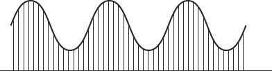
The first stage is sampling. The analogue signal is split up into small samples, the ‘height’ (we should really say amplitude) of which will be measured in the next stage. A very important thing about this sampling process is that it must be carried out at a great rate. In CDs and many other modern digital systems, this rate is just over 44 000 times a second, but 48 000 is also used in some equipment. The vertical lines in Figure 10.1 represent individual samples.

Figure 10.1 Sampling

Quantizing

Next, each sample has to be measured. This is known as quantizing.

Figure 10.2 illustrates a very basic quantizing arrangement. It shows six quantizing levels – and think of these as graduations on a ruler which measures the amplitude of each sample. The system doesn't allow us to use fractions of a division, so the measurements of the signal are going, in this case, to be rather coarse.

The more accurately this amplitude measurement is done, the better the quality of the final result. For real accuracy there needs to be a large number of graduations on this ruler. About 8000 is a usable minimum, but this is not enough for high-quality (e.g. CD quality) recordings, when about 65 000 graduations, or quantizing levels, are needed!

At this point, the brain starts to become bemused by the magnitude of things – measuring the music 44 000 times a second, each measurement being a number between 0 and 65 000! Fortunately, modern electronics can cope with it all fairly easily. Nevertheless, let us pause to see what we're committing the system to. A digital tape or disc must store numbers which can be anything up to 65 000 and do this at a rate of just over 44 000 of them each second!

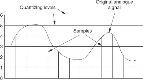
Figure 10.2 A very simple quantizing system

Binary arithmetic

Luckily, things begin to get a little simpler when we cast around for alternative kinds of arithmetic. Digital audio uses binary arithmetic. With our usual day-to-day arithmetic we count from 0 to 9, and then put a 1 in front to go from 10 to 19, then a 2, and so on. In binary arithmetic there are only two digits, 1 and 0, instead of ten, and the counting is from 0 to 1, and then a 1 is put in front to make 10. The next number has one added to make 11 (don't call it ‘eleven’ – it isn't!) and then a further 1 is put in front so that we have 100, 101 and so on. Table 10.1 compares our standard decimal arithmetic with binary. If the reader is unfamiliar with binary arithmetic, an attempt should be made to continue the table.

At first, binary arithmetic can seem very complicated. In fact, this is only because we are not used to it – at least, not most of us. In reality it is much simpler than decimal arithmetic. The entire set of multiplication tables is:

Table 10.1

Decimal	Binary	No. of bits
0	0	1
1	1	1
2	10	2
3	11	2
4	100	3
5	101	3
6	110	3
7	111	3
8	1000	4
9	1001	4
10	1010	4

With 16 bits we can go up to just over 65 000.

Figure 10.3 A binary signal

1 × 0 = 0

and

1 × 1 = 1

The rules of addition and subtraction in binary arithmetic are the same as in decimal arithmetic.

However, let us see where this is getting us – we must not let a study of binary arithmetic, however brief, distract us from the main objective, which is digital audio.

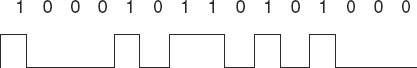
After the quantizing process the resulting numbers are converted into binary, so that, for example, the number 17 832, representing a sample of about a quarter of the maximum height in a CD signal, when converted to binary becomes 100010110101000. Now, if each 1 represents a pulse of voltage we then have the signal shown in Figure 10.3.

This is the sort of code we wanted. Individual pulses can be degraded, but provided they are still just identifiable they can be reconstructed if need be.

Each 1 or 0 in digital audio is called a bit, short for binary digit. Figure 10.3 illustrates a 15-bit number: there are six 1s and nine 0s. The number of bits gives an indication of the quality of the system. CDs use 16 bits. Telephone communication can be satisfactory with fewer than ten.

Regeneration of pulses

Figure 10.4 compares an analogue system with a digital one, both being subjected to interference in each section. The triangular symbols in the analogue chain represent amplifiers. The pulse generators are circuits which detect the presence of a pulse, provided it has not been too badly damaged, and create a new one in its place.

It might seem from what we have been saying that the restoration of digital pulses can go on indefinitely. This is not quite true. Eventually there will be pulses which are too far gone to be regenerated and even though most digital systems make use of error detection and correction – which we shall outline briefly below and explain a little more fully in Part 2 – ultimately there will be perceptible degradation. Nevertheless, digits give a far more reliable and robust way of handling any kind of signal than analogue is ever capable of. It might be worth mentioning that much of the UK's telephone system uses digital signals for distribution – for improved quality and also for economy.

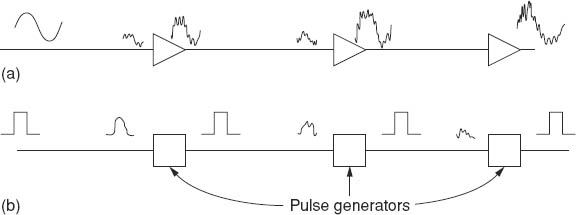
Figure 10.4 Regeneration of (a) analogue signals, (b) pulses in a digital system

Taking a 16-bit system, and with a sampling rate of just over 44 kHz (44.1 kHz in fact), it is possible to achieve a frequency range from as low as we wish up to 20 kHz. The full audio range is easily covered. And when it comes to signal-to-noise ratios, then about 100 dB can be covered. It all seems too good to be true. Not surprisingly there is a penalty and this is the number of bits per second to be handled. Some very simple arithmetic can show this.

Bit rate

With 16 bits for each sample, and about 44 000 samples per second, we have

16 × 44 000 = 704 000 bits/second

And that's for mono! Double the number for stereo and we find that we need 1 408 000 per second or 1.4 megabits/second! We shall later see that there are a lot more data to fit in, such as the error detection we have mentioned, and we can end up with over 4 million bits per second.

Now ordinary analogue tape will record up to 20 kHz, and while it's actually not quite correct to say that the frequency in hertz is precisely the same as bits per second, nevertheless the discrepancy between 20 kHz and 4 MHz is clearly enormous. Conventional tape recording simply cannot cope with digital audio. We will deal with digital tape in the next chapter, but it is enough for the moment to show that a price has to be paid for the potentially high quality that digital audio can provide.

Table 10.2

Original 10-bit sample	Number of 1s	Add parity bit?	New sample	New number of 1s
0011100101	5	Yes	00111001011	6
1100110011	6	No	11001100110	6
0001010110	4	No	00010101100	4
1000100010	3	Yes	10001000101	4

The parity bit is in bold italics.

Error detection

We have already made the point that with analogue systems there is no really effective way of detecting when errors of any kind have occurred.

It's somewhat different with digits. One simple but, with certain limitations, very effective method and one that is widely used is known as parity. What happens is this. Before recording or transmitting a sample, the number of 1s in it is counted and, if necessary, made up to be an even number. A parity bit is added, a 0 if there is already an even number of ones, a 1 if there was an odd number of 1s. Thus, every sample recorded or transmitted contains an even number of 1s.

Suppose an error occurs so that either a 1 is destroyed or a spurious 1 appears where there should be a 0. There will now be an odd number of 1s. So, at the replay or receiving end, when the 1s are counted and an odd number is found in a sample, the system knows that an error has occurred and steps can be taken to reduce the effect. One such step is to repeat the previous sample, and since these are only 1/44 000 second apart, the likelihood is that the deception won't be noticed. Table 10.2 may help to make the parity calculation clear. For simplicity it uses a 10-bit system.

Of course, this puts up the number of bits/second, but only by a small proportion.

Other applications of digital audio

Computer-literate readers will no doubt have already noticed that there is a big similarity between digital audio signals and the electrical pulses used in computers. In that case, couldn't computers be used with digital audio? The answer is yes. In fact, the digital editing mentioned later uses computer technology to perform its task. However, we can go further than that, and it may be sufficient here to do no more than outline some of the processing that can be carried out.

Digital delay

Just as in a computer data can be stored in memory chips, digital audio samples can be stored in chips (for as long as the power is on!). This means that with enough memory a digital signal can be fed into a delay unit and emerge from the output a short time later – from maybe a fraction of a second up to several seconds. The uses for this are many. A short list of applications is:

1.   To add realism in reverberation (see under ‘Artificial reverberation’ below).

2.   As an effect in music (not usually in classical music!) and drama.

3.   To aid in ‘auto double tracking’ (ADT), where a single vocalist is made to appear to sing a duet. A slight delay of a few milliseconds, preferably with an element of pitch change (see below), can be very effective.

4.   To improve intelligibility in PA (public address) work.

5.   To enable what is called a ‘profanity delay’ in some radio phone-in programmes. Everything goes through a delay of perhaps about 15 seconds. If the caller uses unacceptable language the programme presenter presses a button which deletes the contents of the store, including the unwanted words. Clever electronics then builds up the delay gradually, so the fact that there has been some material removed is barely perceptible. It does, though, require a very capable and quick-thinking presenter.

Artificial reverberation

‘Echo’, as it is often termed rather inaccurately, was once created by loudspeakers and microphones in reverberant rooms; later, special steel plates were used and these could be set into vibration electrically to give a very passable imitation of reverberation. Both these methods were bulky and costly.

Cheaper and more compact was the spring reverberator, in which one or more springs were set into vibration by a small transducer fixed to the spring(s) with a further transducer to pick up the reverberations. Very expensive units were reasonably good but the cheap ones sounded like – well – twanged springs!

The advent of digital audio has changed all this. In a digital reverberation device, the incoming digits are stored in memory chips and then released in a very carefully controlled way, so that there is a random and steadily decreasing amplitude of the output.

This can simulate natural reverberation remarkably effectively, and there will normally be control of the reverberation time together with several other characteristics. It becomes possible, then, to produce, within quite wide limits, almost any kind of required reverberation. Modern digital reverberation units can be of comparable cost to a decent cassette machine, and take up less space. There are others, with more comprehensive facilities, which cost ten times as much, but for many purposes the cheap ones can be adequate.

Delay

One way of creating better realism with artificial reverberation is to make use of delays. This may be done with a delay unit as mentioned above, but many digital reverberation devices have variable delays built in. The reason for having a delay is this. The human ear/brain combination is very good at detecting small time intervals, such as those which occur in, say, a room when the ears receive first the direct sound from the source and then the first reflection, as it is called, coming from a wall, floor or ceiling. If the delay between the direct sound and the first reflection is greater than about 40 ms (=1/25 second), then one is aware of a time gap. That is the proper definition of ‘echo’ – when one is aware of a time gap between two sounds.

If this time interval – the initial time delay (which we've already mentioned in Chapter 3) – is less than about 40 ms, the brain does not recognize the gap as such, but is nevertheless subconsciously aware of it and uses the information to assess the size of the room. (Try blindfolding someone and taking them into a room they have not been in before. After a few moments of conversation it will almost always be found that the person can make an approximate judgement of the size of the room.) To recreate a convincing artificial reverberation, then, means using an appropriate time delay as well as the correct reverberation time. To take an example, a large hall will only be fully simulated if a longish reverberation time, perhaps 2 or 3 seconds, is used with an initial time delay of maybe 20 or 30 ms.

Pitch changing

If one imagines digital samples being fed into a set of stores but then taken out at a slightly different rate it will be seen, we hope, that the effect will be to change the pitch of the original. Figure 10.5 shows in simple diagrammatic form the principle of digital pitch changing.

In Figure 10.5, the boxes marked A, B, ..., n represent digital memory stores. Imagine the ‘input electronic switch’ to move round the circle, putting a digital sample into each store in turn. The ‘output electronic switch’ reads the contents of each store and then empties it so that it is ready for another sample. The samples that are read out will ultimately be converted back to analogue signals.

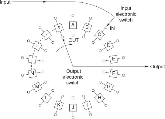
Figure 10.5 Simplified pitch changing

Suppose, though, that the output switch rotates faster than the input one. The effect will be that the pitch of the analogue output will be higher than the pitch of the input. The reader will no doubt wonder how this could be a continuous process because sooner or later one switch will catch up with, or be caught up by, the other! In fact it can't, but with the use of clever technology the impression can be given that it is continuous. The curious and puzzled reader is referred to the ‘Further reading’ section.

MIDI

This stands for Musical Instrument Digital Interface. This really relates to electronic music but a brief mention may not be inappropriate here.

MIDI is not a specific device, but an internationally agreed standard for connecting together two or more electronic instruments. The MIDI link carries information about the times of start and finish of a note, its pitch and other data so that, for example, an electronic organ or an ordinary PC with the right software can ‘trigger’ other equipment. A typical instrument such as a synthesizer may be able not only to generate MIDI data, but also to receive MIDI from another source and then pass it on to a further instrument. The book list at the end suggests suitable further reading.

Data compression

This means reducing the number of bits in an audio sample without a serious reduction in quality. It's made possible by a fairly recent development in digital audio to resort to very clever but legitimate trickery, taking advantage of the characteristics of the human ear.

To begin with there are many ‘sounds’ that we cannot hear: frequencies in the region of 30 Hz unless at a high level, for example. The normal ear is about 70 dB less sensitive to 30 Hz than it is at around 3 kHz and it's not particularly sensitive to the higher audio frequencies above about 3 kHz. Also, certain sounds can be ‘masked’ by others. It has been known for some time that a sound at a particular level can render the ear quite insensitive to nearby frequencies (usually higher) at a lower level.

By making use of circuitry that, as it were, mimics these characteristics of the human ear, it is possible to avoid recording the undetectable sounds. There are various processes. One is known as Precision Adaptive Subband Coding (PASC) or perceptual coding, and it makes it possible to throw away up to about 80% of the original data. Another method, used by MiniDiscs (of which more later) is called ATRAC, which stands for Adaptive Transform Acoustic Coding. MP3 also uses clever data compression.

Additional terminology

Two terms are worth a brief mention:

1.   ADC: analogue-to-digital converter. This is the device (in the form of a chip) which samples the analogue signal and gives a digital output. The complementary device is the

2.   DAC: digital-to-analogue converter, which translates a digital signal back to analogue.

Questions

1.   The sampling rate used in compact discs is approximately how many times per second?

a. 44 000

b. 48 000

c. 65 000

d. 704 000

2.   What would the binary number 1001 represent in ordinary arithmetic?

a. 5

b. 7

c. 9

d. 11

3.   What does MIDI stand for?

a.   Musical Integrated Digital Instrument

b.   Musical Instrument Direct Insertion

c.   Musical Integrated Digital Insertion

d.   Musical Instrument Digital Interface