2

Some technical bits

There are some technical terms that are much bandied about in audio. While it is possible to survive without knowledge of them, they are a great help in making the most of the medium. However, you may wish to skip this chapter and read it later.

2.1 Loudness, decibels and frequencies

How good is the human ear?

Sound is the result of pressure: compression/decompression waves travelling through the air. These pressure waves are caused by something vibrating. This may be obvious, like the skin of a drum, or the string and sounding board of a violin. However, wind instruments also vibrate. It may be blowing through a reed or by blowing across a hole; the turbulence causing the column of air within the pipe of the instrument to vibrate.

The two major properties that describe a sound are its frequency and its loudness.

Frequency

This is a count of how many times per second the air pressure of the sound wave cycles from high pressure, through low pressure and back to high pressure again (Figure 2.1). This used to be known as the number of ‘cycles per second’. This has been given a metric unit name: 1 hertz (Hz) is one cycle per second and is named after Heinrich Hertz who did fundamental research into wave theory in the nineteenth century.

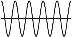
Figure 2.1 Five cycles of a pure audio sine wave

The lowest frequency the ear can handle is about 20 Hz. These low frequencies are more felt than heard. Some church organs have a 16 Hz stop which is added to other notes to give them depth. Low frequencies are hardest to reproduce and, in practice, most loudspeakers have a tough time reproducing much below 80 Hz.

At the other extreme, the ear can handle frequencies of up to 20 000 Hz, usually written as 20 kilohertz (kHz). As we get older, our high frequency limit reduces. This can happen very rapidly if the ear is constantly exposed to high sound levels.

The standard specification for high fidelity audio equipment is that it should handle frequencies between 20 Hz and 20 kHz equally well. Stereo FM broadcasting is restricted to 15 kHz, as is the Near Instantaneously Companded Audio Multiplex (NICAM) system used for television stereo in the UK. But Digital Radio is not, and so broadcasters have begun to increase the frequency range required when programmes are submitted.

The frequencies produced by musical instruments occupy the lower range of these frequencies. The standard tuning frequency 'middle A’ is 440 Hz. The ‘A’ one octave below that is 220 Hz. An octave above is 880 Hz. In other words, a difference of an octave is achieved by doubling or halving the frequency.

Instruments also produce ‘harmonics’. These are frequencies that are multiples of the original ‘fundamental’ notes. It is these frequencies, along with transients (how the note starts and finishes) that give an instrument its characteristic sound. This is often referred to as the timbre (pronounced ‘tam ber’).

Loudness

Our ears can handle a very wide range of levels. The power ratio between the quietest sound that we can just detect – in an impossibly quiet sound insulated room – and the loudest sound that causes us pain is:

1:1000 000 000 000

‘1’ followed by twelve noughts is one million million! To be able to handle such large numbers a logarithmic system is used. The unit, called a bel, can be thought of as a measure of the number of noughts after the ‘1’. In other words, the ratio shown above could also be described as 12 bels. Similarly a ratio of 1: 1000 would be 3 bels. A ratio of 1:1 – no change – is 0 bels. Decreases in level are described as negative. So a ratio of 1000: 1 – a reduction in power of 1/1000th – is minus 3 bels.

For most purposes, the bel is too large a unit to be convenient. Instead the unit used every day, is one-tenth of a bel. The metric system term for one-tenth is ‘deci’, so the unit is called the ‘decibel’. The abbreviation is ‘dB’ – little ‘d’ for ‘deci’ and big ‘B’ for ‘bel’ as it is based on a person's name – in this case Alexander Graham Bell, the inventor of the telephone and founder of Bell Telephones, who devised the unit for measuring telephone signals. Conveniently, a change of level of 1 dB is about the smallest change that the average person can hear (Table 2.1).

Table 2.1 Everyday sound levels

0 dB		Threshold of hearing: sound insulated room
10 dB		Very faint – a still night in the country
30 dB		Faint – public library, whisper, rustle of paper
50 dB		Moderate – quiet office, average house
70 dB		Loud – noisy office, transistor radio at full volume
90 dB		Very loud – busy street
110 dB		Deafening – pneumatic drill, thunder, gunfire
120 dB		Threshold of pain

3 dB represents a doubling of signal power. But human hearing works in such a way that 3 dB does not actually sound twice as loud. For audio to sound twice as loud requires considerably more than a doubling of signal power. A 10 dB increase in signal power is considered to sound twice as loud to the human ear.

2.2 Hearing safety

One of the hazards of audio editing on a PC is that it is often done on headphones in a room containing other people. Research has shown that people, on average, listen to headphones 6 dB louder than they would to loudspeakers. So already they are pumping four times more power into their ears.

When you are editing, there are going to be occasions when you turn up the volume to hear quiet passages and then forget to restore it when going on to a loud section. The resulting level into your ears is going to be way above that which is safe.

Some broadcasting organizations insist that their staff use headphones with built-in limiters to prevent hearing damage. By UK law, a sound level of 85dBA is defined as the first action level (the ‘A’ indicates a common way of measuring sound-in-air level, as opposed to electrical, audio, decibels). You should not be exposed to sound at, or above, this level for more than 8 hours a day. If you are, as well as taking other measures, the employer must offer you hearing protection.

90 dBA is the second action level and at this noise level or higher, ear protection must be worn and the employer must ensure that adequate training is provided and that measures are taken to reduce noise levels, as far as is reasonably practicable.

The irony here is that the headphones could be acting as hearing protectors for sound from outside, but be themselves generating audio levels above health and safety limits.

If you ever experience ‘ringing in the ears’ or are temporarily deafened by a loud noise, then you have permanently damaged your hearing. This damage will usually be very slight each time, but accumulates over months and years; the louder the sound the more damage is done.

Slowly entering a world of silence may seem not so terrible but, if your job involves audio, you will lose that job. Deafness cuts you off from people; it is often mistaken for stupidity. Worse, hearing damage does not necessarily create a silent world for the victim. Suicides have been caused by the other result of hearing damage. The gentle-sounding word used by the medical profession is ‘Tinnitus’. This conceals the horror of living with loud, throbbing sounds created within your ear. They can seem so loud that they make sleep difficult. Some people end up in a no-win situation where, to sleep, they have to listen to music on head-phones at high level to drown the Tinnitus. Of course this, in turn, causes more hearing damage.

The Royal National Institute for Deaf People (RNID) has simulations of Tinnitus on its web site http://www.rnid.org.uk/information_resources/tinnitus/about_tinnitus/what_does_it_sound_like/. This can also be found on this book's CD-ROM.

If you are reading this book then you value your ears; so please take care of them!

2.3 Analog and digital audio

Analog audio signals consist of the variation of sound pressure level with time being mimicked by the analogous change in strength of an electrical voltage, a magnetic field, the deviation of a groove, etc.

The principle of digital audio is very simple and that is to represent the sound pressure level variation by a stream of numbers. These numbers are represented by pulses. The major advantage of using pulses is that the system merely has to distinguish between pulse and no-pulse states. Any noise will be ignored provided it is not sufficient to prevent that distinction (Figure 2.2).

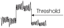
Figure 2.2 Distinction between pulse and no-pulse states

The actual information is usually sent by using the length of the pulse; it is either short or long. This means that the signal has plenty of leeway in both the amplitude of the signal (how tall?) and the length of the pulse. Well-designed digital signals are very robust and can traverse quite hostile environments without degradation.

However, this can be a disadvantage for, say, a broadcaster with a ‘live’ circuit, as there can be little or no warning of a deteriorating signal. Typically the quality remains audibly fine, until there are a couple of splats, or mutes, then silence. Analog has the advantage that you can hear a problem developing and make arrangements for a replacement before it becomes unusable.

Wow and flutter are eliminated from digital recording systems, along with analog artefacts such as frequency response and level changes. If the audio is copied as digital data then it is a simple matter of copying numbers and the recording may be ‘cloned’ many times without any degradation. (This applies to pure digital transfers; however, many modern systems, such as Minidisc, MP3s, Digital Radio and Television, use a ‘lossy’ form of encoding. This throws away data in a way that the ear will not usually notice. However, multi-generation copies can deteriorate to unusability within six generations if the audio is decoded and re-encoded, especially if different forms of lossy compression are encountered. Even audio CD and Digital Audio Tape (DAT) are lossy to some extent, as they tolerate and conceal digital errors.)

What is digital audio?

Pulse and digital systems are well established and can be considered to have started in Victorian times.

Perhaps the best known pulse system is the Morse code. Like much digital audio, this code uses short and long pulses. In Morse these are combined with short, medium and long spaces between pulses to convey the information. The original intention was to use mechanical devices to decode the signal. In practice it was found that human operators could decode by ear faster.

Modern digital systems run far too fast for human decoding and adopt simple techniques that can be dealt with by microprocessors with rather less intelligence than a telegraph operator. Most systems use two states that can be thought of as on or off, short or long, dot or dash (some digital circuits and broadcast systems can use three, or even four, states but these systems are beyond the scope of this book).

The numbers that convey the instantaneous value of a digital audio signal are conveyed by groups of pulses (bits) formed into a digital ‘word’. The number of these pulses in the word sets the number of discrete levels that can be coded.

The word length becomes a measure of the resolution of the system and, with digital audio, the fidelity of the reproduction. Compact disc uses 16-bit words giving 65 536 states. NICAM stereo, as used by UK television, uses just 10 bits but technical trickery gives a performance similar to 14-bit. Audio files used on the Internet are often only 8-bit in resolution while systems used for telephone answering, etc. may only be 4-bit or less (Table 2.2).

Table 2.2 Table showing how many discrete levels can be handled by different digital audio resolutions

1-bit = 2	7-bit = 128	13-bit = 9192	19-bit = 524 287
2-bit = 4	8-bit = 256	14-bit = 16 384	20-bit = 1 048 575
3-bit = 8	9-bit = 512	15-bit = 32 768	21-bit = 2 097 151
4-bit = 16	10-bit = 1024	16-bit = 65 536	22-bit = 4 194 303
5-bit = 32	11-bit = 2048	17-bit = 131 071	23-bit = 8 388 607
6-bit = 64	12-bit = 4096	18-bit = 262 143	24-bit = 16 777 215

The larger the number, the more space is taken up on a computer hard disk or the longer a file takes to copy from disk to disk or through a modem. Common resolutions are: 8-bit, Internet; 10-bit, NICAM; 16-bit, compact disc; 18-24-bit, enhanced audio systems for production. Often, 32-bit is often used internally for processing to maintain the original bit-resolution when production is finished.

On the accompanying CD-ROM there is a demonstration of speech and music recorded at low bit rates; from 8 to 1 bits. There is no attempt to optimize the sound.

Sampling rate

A major design parameter of a digital system is how often the analog quantity needs to be measured to give accurate results. The changing quantity is sampled and measured at a defined rate.

If the ‘sampling rate’ is too slow then significant events may be missed. Audio should be sampled at a rate that is at least twice the highest frequency that needs to be produced. This is so that, at the very least, one number can describe the positive transition and the next the negative transition of a single cycle of audio. This is called the Nyquist limit after Harry Nyquist of Bell Telephone Laboratories who developed the theory.

For practical purposes, a 10 per cent margin should be allowed. This means that the sampling rate figure should be 2.2 times the highest frequency. The 20 kHz is regarded as the highest frequency that most people can hear. This led to the CD being given a sampling rate of 44 100 samples a second (44.1 kHz). The odd 100 samples per second is a technical kludge. Originally digital signals could only be recorded on videotape machines, and 44.1 kHz will fit into either American or European television formats (see box).

The sampling process must be protected from out-of-range frequencies. These ‘beat’ with the sampling frequency and produce spurious frequencies that not only represent distortion but, because of their non-musical relationship to the intended signal, represent a particularly nasty form of distortion. These extra frequencies are called alias frequencies and the filters called antialiasing filters. It is the design of these filters that can make the greatest difference between the perceived qualities of analog to digital converters. You will sometimes see references to ‘oversampling’. This technique emulates a faster sampling rate (4x, 8x, etc.) and simplifies the design of the filters as the alias frequencies are shifted up several octaves.

Errors

A practical digital audio system has to cope with the introduction of errors, owing to noise and mechanical imperfections, of recording and transmission. These can cause distortion, clicks, bangs and dropouts, when the wrong number is received.

Digital systems incorporate extra ‘redundant’ bits. This redundancy is used to provide extra information to allow the system to detect, conceal or even correct the errors. Decoding software is able to apply arithmetic to the data, in real time, so it is possible to use coding systems that can actually detect errors.

However, audio is not like accountancy, and the occasional error can be accepted, provided it is in a well-designed system where it will not be audible. This allows a simpler system, using less redundant bits, to be used to increase the capacity, and hence the recording length, of the recording medium. This is why a Compact Disc Recordable (CDR) burnt as a computer CD-ROM storing wave file data has a lower capacity than the same CDR using the same files as CD-audio. CD-ROMs have to use a more robust error correction system as NO errors can be allowed. As a result a standard CDR can record 720 Mbytes of CD-audio (74 minutes) but only 650 Mbytes of computer data.

Having detected an error a CD player may be able to:

1 Correct the error (using the extra ‘redundant’ information in the signal).

2 Conceal the error. This is usually done either by sending the last correctly received sample (replacement), or by interpolation, where an intermediate value is calculated.

3 Mute the error. A mute is usually preferable to a click.

While the second and third options are good enough for the end product used by the consumer, you need to avoid the build-up of errors during the production of the recording. Copies made on hard disk, internally within the computer, will be error-free. Similarly copies made to CD-ROM or to removable hard disk cartridge, will also have no errors (unless the disk fails altogether because of damage).

Multi-generation copies made through the analog sockets of your sound card will lose quality. Copies made digitally to DAT will be better, but can still accumulate errors. However, a computer backup as data to DAT (4 mm) should be error-free (as should any other form of computer backup medium. These have to be good enough for accountants, and therefore error-free).

How can a computer correct errors?

It can be quite puzzling that computers can get things wrong but then correct them. How is this possible? The first thing to realize is that each datum bit can only be ‘0’ or ‘1’. Therefore, if you can identify that a particular bit is wrong, then you know the correct value. If ‘0’ is wrong then ‘1’ is right. If ‘1’ is wrong then ‘0’ is right.

The whole subject of error correction involves deep mathematics but it is possible to give an insight into the fundamentals of how it works. The major weapon is a concept called parity. The basic idea is very simple, but suitably used can become very powerful. At its simplest this consists of adding an extra bit to each data word. This bit signals whether the number of ‘1’s in the binary data is odd or even. Both odd and even parity conventions are used. With an even parity convention the parity bit is set so that the number of ‘1’s is an even number (zero is an even number). With odd parity the extra bit is set to make the number of ‘1’s always odd.

Received data is checked during decoding. If the signal is encoded with odd parity, and arrives at the decoder with even parity, then it is assumed that the signal has been corrupted. A single parity bit can only detect an odd number of errors.

Quite complicated parity schemes can be arranged to allow identification of which bit is in error and for correction to be applied automatically. Remember that the parity bit itself can be affected by noise.

Illustrated in Figure 2.3 is a method of parity checking a 16-bit word by using eight extra parity bits. The data bits are shown as ‘b’, the parity bits are shown as ‘P’.

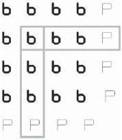
Figure 2.3 A method of parity checking a 16-bit word by using 8 extra parity bits

The parity is assessed both ‘vertically’ and ‘horizontally’. The data are sent in the normal way with the data and parity bits intermingled. This is called a Hamming code. If the bit in column 2, row 2 were in error, its two associated parity bits would indicate this. As there are only two states then, if the bit is shown to be in error, reversing its state must correct the error.

Dither

The granular nature of digital audio can become very obvious on low level sounds such as the die-away of reverberation or piano notes. This is because there are very few numbers available to describe the sound, and so the steps between levels are relatively larger, as a proportion of the signal.

This granularity can be removed by adding random noise, similar to hiss, to the signal. The level of the noise is set to correspond to the ‘bottom bit’ of the digital word. The frequency distribution of the hiss is often tailored to optimize the result, giving noise levels much lower than would be otherwise expected. This is called ‘noise-shaping’. PC audio editors often have an option to turn this off. Don't do this unless you know what you are doing. Dither has the, almost magical, ability to enable a digital signal to carry sounds that are quieter than the equivalent of just 1 bit. There is a demo of dither on this book's CD-ROM.

2.4 Time code

All modern audio systems have a time code option. With digital systems, it is effectively built in, at its simplest level, it is easy to understand; it stores time in hours, minutes and seconds. As so often, there are several standards.

The most common audio time display that people meet is on the compact disc; this gives minutes and seconds. For professional players, this can be resolved down to fractions of second by counting the data blocks. These are conventionally called frames and there are 75 every second. This is potentially confusing as CDs were originally mastered from 3/4 inch U-Matic videotapes where the data were configured to look like an American Television picture running at 30 video frames per second (fps).

In 1967, the Society of Motion Picture and Television Engineers (SMPTE) created a standard defining the nature of the recorded signal, and the format of the data recorded. This was for use with videotape editing. Data are separated into 80-bit blocks, each corresponding to a single video frame. The way that the data are recorded (Biphase modulation) allow the data also to be read from analog machines when the machines are spooling, at medium speed, with the tape against the head, in either direction. With digital systems, the recording method is different but the code produced stays at the original standards.

The SMPTE and the European Broadcasting Union (EBU) have defined a common system with three common video frame standards. 25 fps (European TV) and 30 fps (American Black&White TV). For technical reasons, with the introduction of color to the American television signal there is also a more complicated format known as 30 fps drop frame which corresponds to an average to 29.97 fps. Since the introduction of sound in the 1920s, film has always used 24 fps.

By convention, on analog machines, the highest numbered track is used for time code; track 4 on a 4-track; track 16 on a 16-track, etc. It is a nasty screeching noise best kept as far away from other audio as possible.

Time code can also be sent to a sequencer, via a converter, as MIDI data allowing the sequencer to track the audio tape. The simple relationship between bars, tempo and SMPTE time as shown by sequencers like Cubase is only valid for 120 beats per minute 4/4 time. MIDI time code generators need to be programmed with the music tempo and time signature used by the sequencer, so that they can operate, in a gearbox fashion, so that the sequencer runs at the proper tempo.

People editing audio for CD will often prefer to set the Time Display to 75fps to match the CD data. There is a small technical advantage to ensuring that an audio file intended for CD ends exactly at the frame boundary as the remainder of any unfilled frame will be filled with digital silence (all zeros). You will get a click on the frame boundary as audio silence will not be all zeros.

Right clicking on Adobe Audition 2.0’s time display provides a popup with a wide range of options for the frame dis-play (Figure 2.4) including being able to match to the bars and beats of a MIDI track.

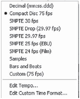
Figure 2.4 Right clicking on Cool Edit's time display provides a wide range of options for the frame display

See Appendix 3 for more information on time code.