9

Audio design

9.1 Dangers

Audio editors come with a multitude of ‘toys’ that you may never need – until that day when they rescue you from certain disaster!

Remember that, just because a toy is available, you do not HAVE to use it. There is no substitute for clear, interesting, relevant speech or good music, well performed. With documentary, have faith in the power of the spoken word. One of the more depressing of my activities as a studio manager was working with producers who did not. They would ruin exciting speech by blurring it with reverberation or obscuring it with sound effects.

All the facilities available allow you, very easily, to ruin recordings. Audio and music technology is full of controls that, set in one direction, do nothing and, set in the other, make everything sound dreadful. Somewhere in between, if you are lucky, is a setting where something magical happens and a real improvement is obtained. When trying to find this setting, always refresh your ears regularly by checking the sound of the recording with nothing done to it.

9.2 Normalization

The first of these toys is normalization, which is so massively useful that you are likely to use it constantly.

One of the very first things that is done when making a recording is to ‘take level’. The recording machine is adjusted to give an adequate recording level with ‘a little in hand’ to guard against unexpected increases in volume. However, that little bit in hand will vary, as will the volume of the speaker or performer.

Most recordists know that people, in general, are 6dB louder on a take than when they give level – except those occasions when they are quieter! The result is that, even for those most meticulous with levels, different inserts into a programme will vary in level and loudness. While level and loudness are connected they are not the same thing.

The three illustrations (Figures 9.1-9.3) show the same piece of audio but at different loudness. Figure 9.1 illustrates audio which is at a lower level (6dB) than the other two. Figures 9.2 and 9.3 are the same level but Figure 9.3 sounds much louder. When we talk about level we actually mean the ‘peak’ level – we talk about audio ‘peaking’ on the meter. On average speech or music most of the time the instantaneous level is much less.

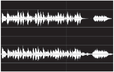
Figure 9.1 Audio at -6dB

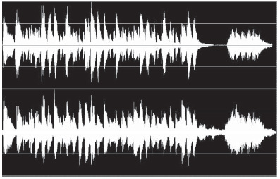
Figure 9.2 Audio normalized to 0dB

Audio, within the computer, is stored as a series of numbers so it is very easy for the computer to multiply those numbers, by a factor, so that the highest number in your audio signal is set to the highest value that can be stored. If this is done to all your audio inserts when you start, this will ensure that your levels are consistent.

However, their relative loudness may not be the same. It all depends on what proportion of your recording is at the higher levels. As a generalization, while the peak level is represented by the highest points reached on the display, the loudness is equivalent to the area of the audio display.

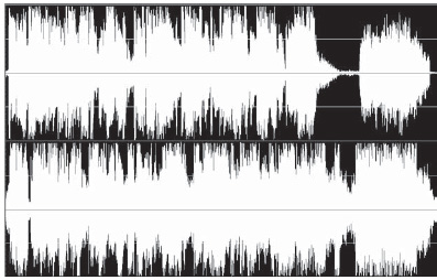
Figure 9.3 Audio compressed to 0dB

Figure 9.3, although showing exactly the same peak level as Figure 9.2, is much louder because it has been compressed.

9.3 Basic level adjustment

Effects/Amplitude/Amplify (Figure 9.4) can be used to change the level of a file or a selection by sliding or typing the figure in.

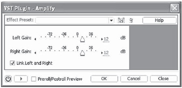
Figure 9.4 Effects/Amplitude/Amplify

Effects/Amplitude/Amplify/Fade (Figure 9.5) does the same thing but can transition from one value to another over the length of the file or selection.

The Effects/Amplitude/Binaural Auto-Panner tweaks the phase of the two channels and rotates sound spatially from left to right in a seemingly circular pattern. This effect delays either the left or right channel so sounds reach each ear at different times, tricking the brain into thinking sounds are coming from either side (Figure 9.6).

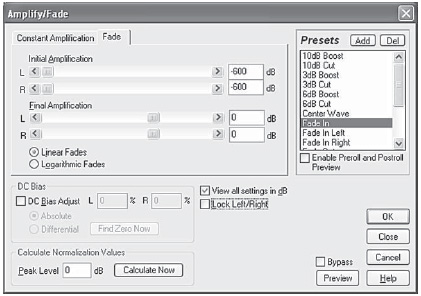
Figure 9.5 Effects/Amplitude/Amplify/Fade

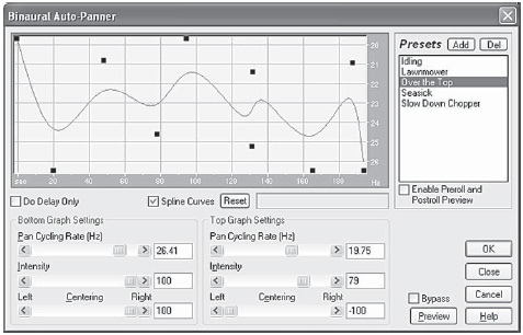
Figure 9.6 Binaural Auto-Panner effect (Edit View only)

Effects/Amplitude/Amplify/Channel mixer (Figure 9.7) facilitates cross mixing between the two stereo channels. The invert options allow you to use phase tricks including generating and decoding MS (Middle-Side) stereo (see Section 9.12 ‘Spatial effects’).

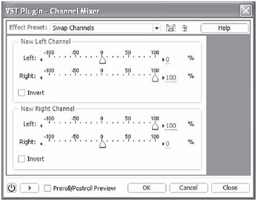
Figure 9.7 Effects/Amplitude/Amplify/Channel mixer

9.4 Compression/limiting

Audio compression varies enormously in what it can do. It is not a panacea, as it can cause audibility problems. Essentially, a compressor is an audio device that changes its amplification, and hence the level, from instant to instant.

You have control over how fast peak level is reduced (attack time). You have separate control over how fast the level is restored after the peak (recovery time). You also have control of how much amplification is applied before compression, by how much the level is controlled, and at what level the compression starts.

The simplest compressor that most people meet is the ‘automatic volume control’ (AVC) used by recording devices ranging from Minidisc and video recorders to telephone answering machines. A professional recorder should give the user the option of bypassing the AVC, to enable manual control of the level.

The AVC has both a slow attack and a slow recovery time. Often it has just two settings (speech and music) with the music setting having even slower attack and recovery times. Even so, modern devices found on such things as Minidisc recorders are often relatively unobtrusive.

The normal advice, with analog recording, is not to use AVC where the resulting recording is going to be edited. This is because the background noise goes up and down at the same time and any sudden change at an edit will be very obvious. With digital recording and editing the arguments are more evenly balanced, especially when digital editing is being used.

Analog recorders overload ‘gracefully’ and the increase in distortion is relatively acceptable, for short durations. Digital recorders are not so forgiving. They record audio as a string of numbers and have a maximum value of number that they can record. This corresponds to peak level on the meter.

The CD standard, also used by Minidisc and DAT, is 16 bit, which allows 65 536 discrete levels occupying the numbers +32 768 through 0 to –32 767. Any attempt to record audio of a higher level than this will cause a string of numbers set at the same peak value. When played back, this produces very nasty clicks, thumps or grating distortion.

When recording items like vox pops, by the very nature of an in-the-street interview, there is likely to be a very high background noise. This has always been a classic case where switching off any AVC was regarded as essential, because of the resulting traffic noise bumps on edits. However, the likelihood of short- or medium-term overload is quite considerable. On the other hand, sudden short, very high-level sounds such as exhaust backfires and gunshots can ‘duck’ the AVC to inaudibility for several seconds.

Digital editors make matching levels at edits the work of seconds. The danger of overload is such that this correction may be preferable to risking losing a recording owing to digital overload. In reality, it is down to the user to decide how good their recording machine's AVC is compared with how well it copes with overloads. They may prefer deliberately to underrecord, giving ‘headroom’.

Most portable recorders have some form of overload limiting which may allow you to return to base with ‘usable’ recordings, but it is better to return with good recordings. In the end, a saving grace is that it is the nature of these environments that the background noise is quite high and will drown any extra noise from deliberately recording with a high headroom.

Compression may make the audio louder, but it also brings up the background noise rather more than the foreground. This can mean that noise that was not a problem, becomes one. It will also bring up the reflections that are the natural reverberation of a room. This can change an open, but OK, piece of actuality into something that sounds as if the microphone had been lying on the floor pointing the wrong way.

If you are creating material for broadcast use you should also be aware that virtually all radio stations compress their output at the feed to the transmitter. While the transmitter processors used are quite sophisticated, they will be adding compression to any you have used. This can mean that something that sounds only just acceptable on your office headphones may sound like an acoustic slum on air.

There are standard options on any compressor that are emulated in any compression software. The compressor first amplifies the sound and then dynamically reduces the level (compression software is often found in the menu labelled as ‘Dynamics’). Compressors can be thought of as ‘electronic faders’ that are controlled by the level of the audio at their input. With no input or very quiet inputs they have a fixed amplification (gain), usually controlled by separate input and output gain controls. Once the input level reaches a threshold level, their amplification reduces as the input is further increased. The output level still increases, but only as a set fraction of the increase in input level. This fraction is called the compression ratio (Figure 9.8).

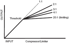
Figure 9.8 Compression ratios

A compression ratio of 2:1 means that once the audio is above the threshold level then the output increases by 1 dB for every 2 dB increase in input level.

A ratio of 3:1 means that once the audio is above the threshold level then the output increases by 1 dB for every 3 dB increase in input.

Compression ratios of 10:1, or greater, give very little change of output for large changes of input. These settings are described as limiting settings and the device is said to be acting as a limiter.

Hard limiting

Hard limiting can be useful to get better level out of a recording that is very ‘peaky’. Some people have quiet voices with some syllables being unexpectedly loud. Hard limiting can chop these peaks off with little audible effect on the final recording, except that it is now louder. Adobe Audition 2.0 has a separate effects transform for this.

Threshold

The Threshold control adjusts at what level the compression or limiting starts to take place. By the very nature of limiting, the threshold should be set near to the peak level required. With compression, it should be set lower; 8dB below peak is a good starting place.

Attack

Control for adjusting how quickly the gain is reduced when a high-level signal is encountered. If this is set to be very short then the natural character of sounds is softened and all the ‘edge’ is taken out of them. It can be counterproductive as this tends to make things sound quieter. Set too slow an attack time and the compression is ineffective. A good place to start when rehearsing the effect of compression is 50 milliseconds. With musical instruments much of their character is perceived through their starting transients. Too much compression with a poor choice of attack time can make them sound wrong. On the other hand, a compressor set with a relatively slow attack time can actually improve the sound of a poor bass drum by giving it an artificial attack that the original soggy sound lacks.

Release/recovery

These are alternative names for the control that adjusts how fast the gain is restored once the signal is reduced. Set too short and the gain recovers between syllables giving an audible ‘pumping’ sound which is usually not wanted. This makes speech very breathy. A good starting point is 500 milliseconds to 1 second.

Input

Adjusts the amplification before the input to the compressor/limiter part of the circuit. With software graphical display controls this may, at first, appear not to be present but is represented by the slope of the initial part of the graph.

Output

Adjusts the amplification after the compressor/limiter part of the circuit. Because it is after compression has taken place it also appears to change the threshold level on the output. Software compressors often have the option automatically to compensate for any output level reduction due to the dynamic gain reduction, by resetting the output gain.

In/out, bypass

A quick way of taking a device out of the circuit for comparison purposes.

Link/stereo

Two channels are linked together for stereo so that they always have the same gain despite any differences in levels between the left and right channels. If this is not done then you may get violent image swinging on the centre sounds such as vocals.

9.5 Expanders and gates

Adobe Audition 2.0’s dynamics can also act as expanders and gates. These work in a very similar way to compressor/limiters but have the reverse effect. With high-level inputs they have a fixed maximum gain. Once the input level decreases to a threshold level then their gain decreases as the input is further decreased. When used as expanders the output levels still decrease but only as a set fraction of the decrease in input level. This fraction is called the expansion ratio (Figure 9.9).

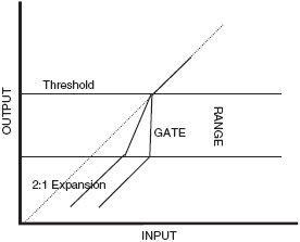
Figure 9.9 Expander and gate actions

A expansion ratio of 2:1 means that once the audio is below the threshold level then the output decreases by 2 dB for every 1 dB decrease in input level. A ratio of 3:1 means that the output decreases by 3 dB for every 1 dB decrease in input. Expansion ratios of 10 : 1 or greater give a very large change of output for little changes of input and the device is said to be acting as a gate.

Unlike compressors, which were originally developed for engineering purposes, the expander is an artistic device and must be adjusted by ear. Changing its various parameters can dramatically change the sound of the sources. Its obvious use is for reducing the amount of audible spill. This is usually restricted by the fact that too much gating or expansion will change the sound of the primary instrument. However, this very fact has led to gates and expanders being used deliberately to modify the sounds of instruments – particularly drums. Their use is almost entirely with multitrack music; bass drums are almost invariably gated.

Expanders and gates are bad news for speech. They change the background noise. The ear tends to latch on to this rather than listening to what is said. While I can imagine circumstances where they might help a speech recording, I have not yet met any.

Dynamics transform (Figures 9.10-9.13)

Adobe Audition 2.0’s Dynamics transform is a very flexible implementation of dynamics control. It provides you with alternative ways of inputting what you want, along with a profusion of presets. A tour through these will educate your ears as to what can be done. There are four tabbed pages within the dialog box; ‘Graphic’, ‘Traditional’, ‘Attack/Release’ and ‘Band Limiting’. The first two tabs give you alternative ways of entering what you want. All four tabs allow you access to the presets.

With the graphical tab (Figure 9.10) you can ‘draw’ the dynamics that you want. Click on the line to give you a ‘handle’ and then move it where you want. It is usually quicker to start from a preset and adjust the settings if required. Illustrated is a ‘soft knee’ compression of the sort associated with the dbx company.

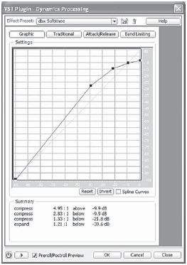
Figure 9.10 Graphic

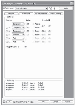
Figure 9.11 Traditional

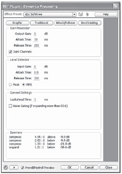
Figure 9.12 Attack/release

Figure 9.13 Band limiting

Figure 9.11 shows the same setting in the ‘Traditional’ tabbed page, with each section labelled as text. ‘Output compensation allows you to boost the level after compression, if this is needed.

Figure 9.12 is where you can setting the attack and release times. How you set these times will substantially affect the sound of an instrument as it will modify its start and finish transients. A very quick recovery time with compression will bring up background noise and increase the apparent amount of reverberation.

Figure 9.13, ‘Band Limiting’ allows you to restrict the frequency range that limiting occurs. The setting shown is one that is used in one of the ‘De-essing’ presets. De-essers do what you would think they reduce the level of sibilants, ‘S’ sounds in a vocalist's voice. You should apply this after any full frequency range compression as otherwise the compression can restore the sibilance!

9.6 Multiband compressor

Adobe Audition 2.0 has a full scale multiband limiter of the sort often used to make CDs and broadcasts sound louder. They split the audio into bands and separately compress each band.

The one supplied with Audition has four bands. (Figures 9.14 and 9.15)

The controls can be a bit overwhelming at first so begin familiarizing yourself by trying the various presets. You can hear what is being done by soloing each band with the ‘S’ button or you can bypass it altogether with the ‘B’ button. You can apply the multiband compression in real time during a mix – conveniently it can be inserted into the main bus – or you can apply it to the mixdown afterwards in the edit view when the controls at the bottom will appear.

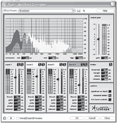
Figure 9.14 Multiband compressor

This is probably the prettiest of the Adobe Audition 2.0 displays and there is certainly a lot going on. The panel is dominated by the spectrum display at the top with the output level and gain control at the top. Three vertical white lines indicate the crossover between bands. They can be slid with the mouse or the numbers typed or dragged beneath. You might expect the lines to be in the centre of the spectrum for each band but this is not apparent because the frequency display is logarithmic. Each band has its own control panel with an output level meter, a threshold control and a gain reduction meter which operates downwards. There are numerical boxes for threshold (working with the slider) gain, compression ratio, attack and release times.

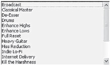
Figure 9.15

Beware of being seduced by multiband processing; it makes for a forward impressive sound and make for extra clarity in difficult listening conditions such as in an automobile. However, it is surprising how often something that impresses for 5 minutes becomes tiring and headache-inducing in 30 minutes.

Tube-modelled compressor

The ‘tube-modelled’ compressor tries to simulate the old valve (vacuum tube) devices. It is bought in from the same company that provides the multiband compressor and has an identical control panel to a single band of its brother. It is actually configured as a VST plug in and can be found using the Effects/VST menu selection (Figure 9.16).

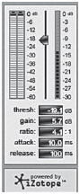
Figure 9.16 Normalize

Normalize

It make sense to normalize files before working on them. Normalization is explained in Chapter 4.

Pan/Expand

This allows you to change the width and pan settings of a file. Its basically an MS control which can pan the M signal and change the level of the S signal (see Section 9.12 ‘Spatial Effects’) (Figure 9.17).

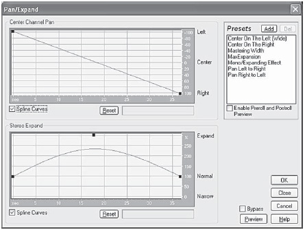
Figure 9.17 Pan/Expand

The stereo expander option (Figure 9.18) is a non-dynamic version which applies a constant change throughout a files or selection.

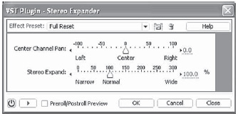
Figure 9.18 The stereo expander option

The stereo field rotate has two options, process and nonprocess. The VST plug-in version can be used as a real-time effect in the multitrack view and be controlled by an automation lane. The process version can be varied over the length of a file in Edit view and then fixed by saving the file (Figure 9.19).

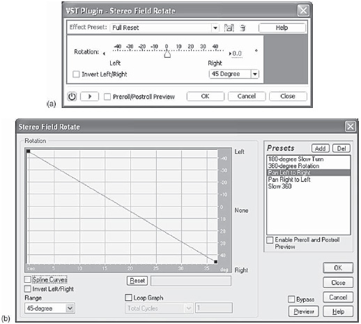
Figure 9.19 The stereo field rotate

9.7 Reverberation and echo

Reverberation (often abbreviated to ‘reverb’) and echo are similar effects.

Echo is a simpler form where each reflection can be distinctly heard (Echo … Echo … Echo … Echo). Reverberation has so many different reflections that it is heard as a continuous sound. For reasons more owing to tradition than logic, broadcasters often refer to reverberation as ‘echo’ and use the term ‘flutter echo’ for echo itself.

Reverberation time

The amount of reverberation is usually quoted in seconds of reverberation time. This is defined as the time it takes for a pulse of sound (such as a gun shot) to reduce (or decay) by 60 dB. This ties in well with how the ear perceives the length of the reverberation.

Diffusion

Simulates natural absorption so that high frequencies are reduced (attenuated) as the reverb decays. Faster absorption times simulate rooms that are occupied and have furniture and carpeting, such as night clubs and theatres. Slower times (especially over 1000 milliseconds) simulate rooms that are emptier, such as auditoriums, where higher frequency reflections are more prevalent. In acoustic environments, higher frequencies tend to be absorbed faster than lower frequencies.

Perception

Adds subtle qualities to the environment by changing the characteristics of the reflections that occur within a room. Lower values create smoother reverb without as many distinct echoes. Higher values simulate larger rooms, cause more variation in the reverb amplitudes, and add spaciousness by creating distinct reflections over time (Figure 9.21).

Devices

Reverb is the first and oldest of studio special effects. Originally it was created by feeding a loudspeaker in a bare room and picking up the sound with a microphone (Figure 9.20). Although this worked, there was no way of changing the style of reverberation. It was also prone to extraneous noises ranging from traffic, hammering, underground trains or even telephones ringing inside the room.

The next development was the ‘echo plate’. A large sheet of metal (the plate) about 2 m x 1m was suspended in a box. There was a device to vibrate the plate with audio and two pickups (left and right for stereo) to receive the reverberated sound.

This worked on a similar principle to a theatre ‘thunder sheet’. The trick was to prevent it sounding like a thunder sheet! This was achieved by surrounding it with damping sheets. By moving these dampers away from the sheet, you would increase the reverberation time (usually at the cost of a more metallic sound). Often, a motor was fitted allowing remote control. In a large building with many studios, a handful of the devices could be shared using a central switching system.

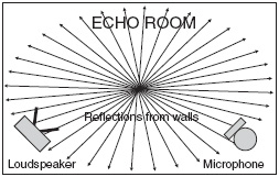
Figure 9.20 ‘Echo’ Room set-up

Devices were also made using metal springs. Their quality was often not good but they took up little space and were ‘good enough’ for many purposes like reverb on disc jockeys on Hallowe'en.

Digital

These days digital reverberation devices reign supreme. The software used on these machines is equally able to be written for use on a PC. Like the separate devices it emulates, the PC will usually offer a number of different ‘programs’ with different acoustics (Figure 9.22). This will often include emulation of the old plates and room, but also include concert hall acoustics, along with special effects that could not exist in ‘real life’.

Reverberation is a complex area as it triggers various complex subconscious cues in the brain. There are two main pieces of information we get from how ‘echoey’ a recording of someone speaking, or talking, is. They both interact, but need separately to be controlled. These are the size of the room, and how far away from the microphone the voice is. Move the voice further from the mic and the more echoey the recording becomes. If the microphone is held and the person walks into a larger room, the more echoey it becomes. However, we are also adept at distinguishing between different types of room. We can hear the difference between an underground car park and a concert hall, a hallway from a living room. How do we do this?

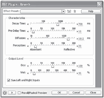
Figure 9.21 Reverb dialog giving the simplest of options

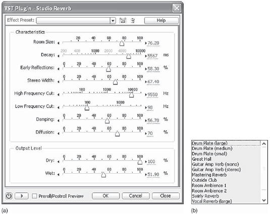
Figure 9.22 Studio Reverb dialog from Adobe Audition 2.0 showing presets.

Let us imagine we are recording in the centre of a large, open acoustic, suspended in the air, as well as centred over the floor. Now make a sharp impulsive noise like a single hand clap, while making a recording. When we examine the waveform of the recording we will see that there is a moment of silence between the hand clap and the start of the reverberation. This is because reverberation is caused by sound reflecting off surfaces such as walls, floors and ceilings. Sound does not travel instantaneously. Its actual speed varies with the temperature and humidity of the air (one of the reasons, the acoustic of a hall can change so dramatically once the audience arrives, even if the seats have been heavily upholstered to emulate the absorption of a person sitting in them). Sound travels at roughly 330 metres per second, or about 1 foot per second. This means that if the nearest reflecting surface is 50 feet away then you will not hear that first reflection for 100/1000th of a second (100 milliseconds). It is the size of this delay that is our major cue for perceiving how large a room a recording was made in. An unfurnished living room may be as reverberant as a cathedral but it will have short delay on the reflections from the walls (10-20 milliseconds) and so can never be confused with the church.

Returning safely to floor level, we can make another recording, with someone speaking and moving towards, and then away from, the microphone. The microphone picks up two elements of the voice (as opposed to the ambient background noise from the environment). These elements are the sound of the voice received directly and the sound received indirectly via reflections.

As the voice moves nearer to, and further from, the microphone, the amount of indirect sound does not really change in any practical way. However, the voice's direct level does change. It is very easy to imagine that it is the reverberation that is changing. This is because a recordist will be setting level on the voice. As it gets closer so the louder it will become. The recordist compensates by turning down the recording level and so apparently reduces the Reverb.

Theoretically, every time the distance from the microphone is doubled, the level will drop by 6 dB.

This is often known as the inverse square law. While this is true for an infinitely small sound source in an infinitely large volume of air, this is not totally true for real sound sources. A person's voice, for example, comes not only from their mouth but from their whole chest area. Only the sibilants and mouth noises (like loose, false teeth and saliva) are small so they disappear much faster than the rest of the voice (one reason why mic placement can be so critical).

As a generalization, if the delays on the reflections remain the same, then the ear interprets relative changes in Reverb level as movement of the sound source relative to the microphone. If the delays change then the ear interprets this as the mic moving with the voice into a different acoustic.

The reason why reflections die away is that only a fraction of the energy is returned each time. Hard stone surfaces reflect well; soft furnishings and carpets do not. Such things as good quality wallpaper on a hard surface will absorb high frequencies but reflect low frequencies as well as does the bare hard surface.

Another reverberation parameter is its smoothness. Lots of flat surfaces give a lumpy, hard quality of reverberation. A hall full of curved surfaces, heavily decorated with carvings, will give a much smoother sound. This does much to explain why many nineteenth-century concert halls sound so much better than their mid-twentieth-century replacements, built when clean, flat surfaces were fashionable. So much more is now known about the design of halls that there is little excuse for getting it wrong in the twenty-first century.

When creating an artificial acoustic, all these mistakes are yours to make! As always with audio processing, it is always very easy to make a nasty ‘science fiction’ sound, but so much more difficult to create something magical and beautiful. The effects transforms within all good digital audio editors are provided with presets. It saves time to use them albeit modifying them slightly. When you find a setting that you really like, you can save it as a new preset.

Summarizing, a simple minimalist external reverberation device would include options such as:

1 Program: Setting the basic simulation; reverb-plate, garage, concert hall, etc.

2 Predelay: This controls how much the sound is delayed before the simulated reflections are heard. This normally varies from zero to 200 milliseconds. As sound travels at approximately 1 foot per millisecond (1/1000th of a second), a predelay of 200 milliseconds (1/5th second) will emulate a large room with the walls 100 feet (30 metre) away (200 feet there and back).

3 Decay: This controls the reverberation time. This is the apparent ‘hardness’ or ‘softness’ of a room. A room with bare shiny walls will have a long reverberation time. A room with carpets, curtains and furniture will have a short Reverb time.

4 High Frequency rolloff: This is an extra parameter that shortens the Reverb time for the high frequencies only, making the ‘room’ seem more absorbent and well furnished.

5 Input and output: Adjusts the input or output level.

6 Mix: Controls a mix between reverberation and the direct sound you are starting with. Sometimes, there are separate controls labelled ‘dry’ and ‘wet’. As a dry acoustic is one without much reverberation, so pure reverberation is thought of as the wet signal.

Let us now take a closer look at how Adobe Audition 2.0 implements this. Reverberation and echo comes under the submenu of delay effects and the choice is potentially overwhelming! (See Figure 9.23.)

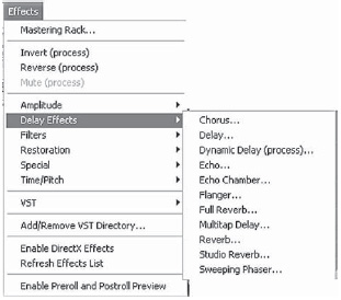
Figure 9.23 Delay Effects submenu.

Chorus (Figure 9.24)

This is an effect used a great deal in pop music. By producing randomly delayed electronic copies of a track, it can make one singer sound like several or many. It can also be used to thicken musical tracks and other sounds. The random delays inherently cause a random pitch change. This can sound very nasty especially on spill behind a vocal.

Outside of music, chorus is not particularly useful except that the various options provided by chorus can produce interesting stylized acoustic effects, not dissimilar to adding echo. The variable delay pitch variation can help produce effects suitable for science fiction. As well as the pitch changing caused by the variable delay, the vibrato settings introduce random amplitude changes.

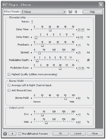
Figure 9.24 Plug-in Reverb

Rather than me trying to describe all the effects, try changing them yourself using the demo version of Adobe Audition 2.0 on the CD supplied with this book. Using a recording of a single voice, give yourself a tour of the preset effects using the preview button. There will be sounds there you will find useful one day.

Delay (Figure 9.25)

This effects transform is the equivalent of tape flutter echo where the output of the playback head was fed back to the record input. While not the most subtle effect, it does have its uses. Emulating Railway station announcements and 1960s Rock ‘n’ Roll come to mind. Again, give yourself a tour around the presets. Used as a real-time effect in the multitrack view Delay's parameters can be controlled by envelopes. With the parameter box displayed in the effects rack you can see the sliders moving in response to the envelope settings as you play though the session.

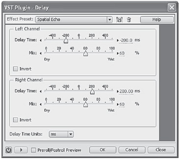
Figure 9.25 Delay effect

Dynamic Delay (Figure 9.26)

The Dynamic delay effects transform allows you to flange the sound in a graphically controlled way. By varying the delay between the original and a copy you get a comb filter effect; the ‘psychedelic’ sound associated with 1960s pop music. This is a ‘Process’ effect that has to be applied to a file and cannot be used in real time.

In those days the only practicable way of apply variable delays was to feed the music to be treated to two identical tape recorders and combine the outputs of the two playback heads. Because of small mechanical imperfections, the two delays introduced by the replay heads were very slightly different. They would vary slightly as the tension varied slightly and changed the stretch of the tape. This became known as phasing. It causes a notch in the frequency response giving a drainpipe type sound as shown in Figure 9.27-9.29. This is because the two signals cancel where half the recorded wavelength of the audio becomes equal to the delay. Depending on the delays involved, not only will the frequency cancelled-out change but there may well be a multiplicity of cancellations producing what is known as a comb filter effect.

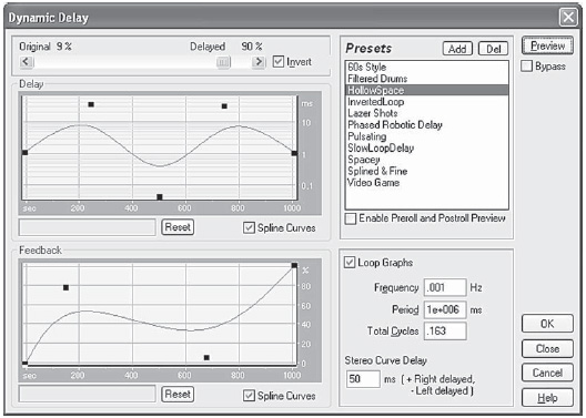
Figure 9.26 Dynamic Delay

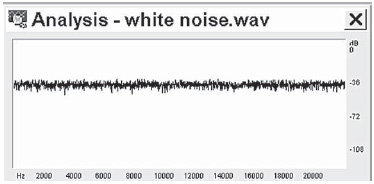
Figure 9.27

According to legend it was John Lennon of The Beatles who found that the delay difference could be modified subtly and controllably by putting a finger on the flange of the feed spool of one of the tape recorders. The effect became known as flanging. It gives the classic skying sound of the 1960s. This is a comb filter effect moving up and down the sound spectrum (Figure 9.30).

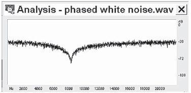
Figure 9.28

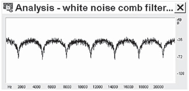
Figure 9.29

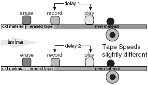
Figure 9.30 Original tape phasing

Echo (Figure 9.31)

This is very much like the delay effects transform with the additional option of adding equalization (EQ) to the delayed echo. Again some useful presets are supplied.

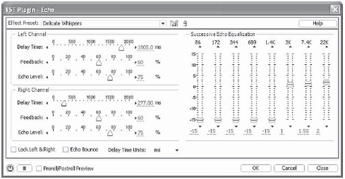
Figure 9.31 Echo

Echo chamber (Figure 9.32)

This approaches designing a reverberant effect in a totally different way.

You are invited to enter the dimensions of the room you wish to simulate and where the microphone is placed. You can also set the absorption (damping factor) of the floor, ceiling and each wall. Some useful dramatic environments are supplied as presets.

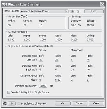
Figure 9.32 Echo chamber

Flanger (Figure 9.33)

As already described in the section above on Dynamic delay. Flanging was so named because the cancelled frequencies could be changed dynamically by pressing a finger on the flange of the feed spool on one of the tape machines. The resulting ‘skying’ effect is irretrievably associated with late 1960s pop music. Both phasing and flanging are available and have their own useful presets.

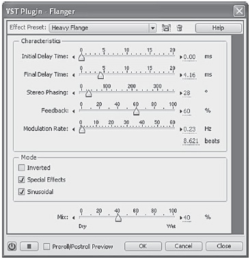
Figure 9.33 Flanger

Full Reverb (Figure 9.34)

This is the all-singing, all-dancing Reverb option. Because of its complication, I do not recommend using this unless you have a specific need and have the time and knowledge to navigate around the options. However, as before, there are some presets that you may find useful.

There are two pages for settings (the vital ones controlling the level of the original signal (dry), early reflections and the Reverb (wet) are repeated on each page). The first page, ‘general’, contains the basic level controls. Section 1 has the reverb settings; Section 2 sets the early reflections which are so critical in our ‘picture’ of the simulated room, effectively controlling the room size.

The other page, ‘coloration’, gives you the ability to equalize the Reverb within the algorithm. You can move the three bands, low, mid and high, around the frequency band. The amount of coloration is adjusted by the three sliders.

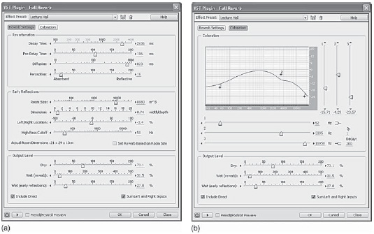
Figure 9.34 Full Reverb

You can separately control the wet/dry mix of the general reverb and the short reflections in the third panel which appears on both pages. As with the other effects transforms, the easiest approach is to use the presets and then modify as required.

Multitap delay (Figures 9.35 and 9.36)

This simulates the old tape loop delay systems. The effects produced are relatively primitive but suit certain types of music or stylized effects.

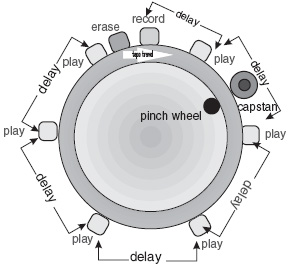
Figure 9.35 Multitap tape delay

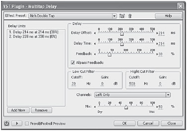
Figure 9.36 Multitap Delay

Reverb (Figure 9.37)

This is the most useful general purpose reverberation effects transform. It is flexible, but still simple to operate. As well as a sensible range of presets, the Reverb effects transform has the basic logical controls. This is the effects transform to use if you ‘just want a bit of reverb’ and you are not too critical as to subtlety.

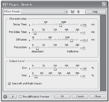
Figure 9.37 Reverb

Studio Reverb (Figure 9.38)

Yet another reverb option. This has a useful reverberation stereo width option. We are so used to hearing music in stereo these days that it is very easy to forget that music that is broadcast will also be heard in mono by many listeners. This is obtained by summing the left and right signals. Out-of-phase material is lost. The width of stereo reverb is caused by out-of-phase audio. This means that if the reverb is very wide then it will reduce in level in mono making the balance sound drier in mono. Slightly narrowing the reverb is a common trick used by broadcast balancers to preserve compatibility so the stereo and mono balances do not differ in liveliness.

Figure 9.38 Studio Reverb

Plug-in Reverb (Figure 9.39)

You can also buy or download reverberation plug-ins with different sound and quality. Adobe Audition 2.0 can handle both the main systems; DirectX and VST. Illustrated in Figure 9.39 is the free ‘Freeverb VST’ plug-in.

Many of the DirectX plug-ins can be downloaded from the Internet in demo versions like the Arboretum Hyperprism plug-in (Figure 9.40). These demos allow you to hear them to check that they do what you want. It's worth saying not all are better, or even, as good as those already built-in to Adobe Audition 2.0. The demos are invariably limited in some way. Some only allow a certain number of uses, a limit to the number of days they work or they put random bleeps into their output so that they cannot be used in a practical way.

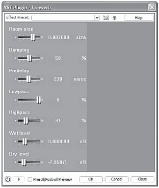
Figure 9.39 Freeverb plug-in reverb

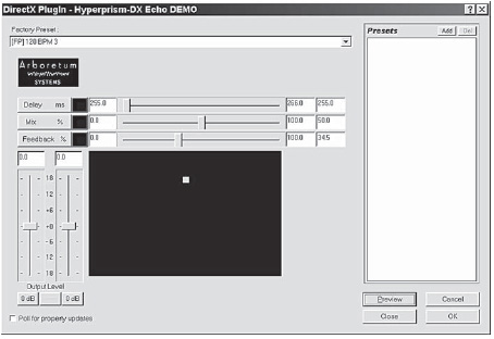
Figure 9.40 Hyperprism echo demo

Phaser (Figure 9.41)

This is very similar to the flanger but with much more control over the effects available.

Again, start by using the presets and play with the settings to modify the sounds.

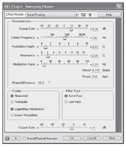
Figure 9.41 Phaser

9.8 Filters

Center Channel Extractor (Figure 9.42)

Adobe Audition 2.0 has almost an embarrassment of EQ and filters. The first on the Effects/filters sub menu is a peculiar one and is an attempt at ‘unmixing’. This is not really possible as it would involve changing the laws of physics but, in audio, we are rarely dealing with perfection but the art of the possible. Adobe Audition's Center Channel Extractor is a tool to help reduce or boost sounds in a stereo mix. The greatest demand is to alter the relative levels of the vocals. The convention is that they are in the centre but Audition's tool also has the ability to tweak for offset audio using either the drop down at the top of the dialog or sliding the values underneath. A need for what this filter supplies indicates a degree of desperation. However, it can get you out of a jam. While the output may often be a bit flakey, it is surprising what you can get away with if it becomes a new element of a mix.

Equalization, or EQ, as it is usually referred to, has two functions. The first is to enhance a good recording and the second, to rescue a bad one.

The best results are always obtained by first choosing the best microphone and placing it in the best place. This is not always possible and so, in the real world, EQ has to come to the rescue.

The most common need for speech EQ is to improve its intelligibility. A presence boost of 3-6 dB around 2.8 kHz usually makes all the difference. Here the simple graphic equalizer effects transform will be fine.

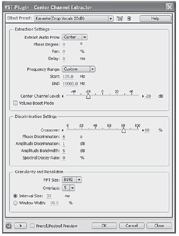
Figure 9.42 Center Channel Extractor

Another common problem is strong sibilance where ‘S's are emphasized; reducing the high frequency content can be advantageous (another option is to use the De-essing preset in the Amplitude/dynamics preset. This has the effect of reducing the high frequencies only when they are at high level).

Bass rumbles are usually best taken out by high-pass filters. This naming convention can be confusing, at first, as it has a negative logic. A filter that passes the high frequencies is not passing the low frequencies! Therefore a high-pass filter provides a bass cut, and a low-pass filter provides a high frequency cut. This sort of filter works without changing the tonal quality of the recording.

As always, it is best to avoid the problem in the first place. If your recording environment is known to have problems with bass rumbles, like the Central London radio studios which have underground trains running just below them, then use a microphone with a less good bass response. A moving coil mic will not reproduce the low bass well, unlike an electrostatic capacitor microphone.

Dynamic EQ (Figure 9.43)

This effect allows you to vary the effect over the selection. There are three graphs selected by the tabs at the top. The first tab allows you to vary the operating frequency with time. The second, the gain and the third the ‘Q’ or bandwidth. Three type of filter are provided low, band and high pass. The first and last terms can be confusing. A ‘low-pass’ filter removes high frequencies (and passes low frequencies). Similarly a ‘high-pass’ filter does the opposite; it passes high frequencies and therefore filter out low frequencies. A band-pass filter passes frequencies within its range while filtering those outside. It can be thought of as a ‘middle-pass’ filter although it can also be used at the extremes of the frequency range. This is a process effect and cannot be used as a real-time multitrack effect.

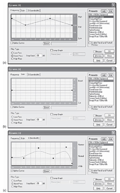
Figure 9.43 Dynamic EQ

FFT filter (Figure 9.44)

FFT stands for Fast Fourier Effects transform. It is nothing less than the Techie's dream of designing a totally bespoke filter. Great fun if you know what you are doing. Totally confusing if you do not! Possibly best avoided if you did not start your career as a technician.

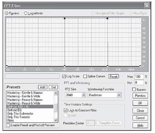
Figure 9.44 FFT filter

Designing your own filter does not need any mathematical ability but you have to have some idea what frequencies you want to filter. You can literally design a filter to remove frequencies that have broken through on to your recording at a gig. You do this by drawing the frequency response that you want. The line on the graph is modified just like the envelopes on the multitrack mixer. Click on the line to create a ‘handle’ and then use the mouse to move it. If the spline curves box is ticked then a smoother curve is achieved with the handles acting more as though they are attracting the line toward themselves rather than actually being ‘fence posts’ on the line.

The windowing functions are different ways of calculating the filters. There is a trade-off between accuracy in generating the curve and artefacts that can spoil the sound. Adobe recommend the Hamming and Blackman functions as giving good overall results.

You can also set up two different filter settings and automatically get a transition between them. This will either be a cross fade between the two settings or if the ‘morph’ box is ticked the settings will gradually change. This means that if you have a transition between a lot of bass boost and a lot of top boost, morphing will cause the boost, as Syntrillium used to describe it, to ‘ooze’ along the frequencies between one and the other. With the box unticked the frequencies between are not affected. The precision factor controls how large the steps are in the transition a higher number means smaller steps but more processing time.

The FFT size controls the precision of processing higher number giving better resolution but slower processing time. Setting to a low value like 512 gives speed when previewing and listening to how your do-it-yourself filter performs. When you actually want to run the filter set to a higher value for better results. Adobe recommend values from 1024 to 8196 for normal use. The power of 2 values in the drop down are the only ones that will work.

For the best results, filter using 32-bit samples. If your source audio is less than this then convert the file to 32 bit to do the filtering, and when done, you can convert back to the lower resolution. This will produce better results than processing at lower resolutions, especially if more than one transform will be performed on the audio. This is because higher resolution mathematics will be used for the 32-bit file and more accurate results obtained.

Graphic equalizer (Figures 9.45)

This effects transform emulates the graphic equalizer often found on Hi-Fi amplifiers. Rather than just offering the five or six sliders of the average Hi-Fi, it gives you a choice of 10, 20 or 30 sliders. Each covers a single frequency band. The more sliders, the better the resolution. It represents a more friendly way of designing your own frequency response. It works rather better than analog equivalents as it does not suffer from the analog system's component tolerances. The illustrations show a setting for a typical presence boost using 10 or 30 sliders.

‘Range’ defines the range of the slider controls. Any value between 4 and 180 dB can be used. (By comparison, standard hardware equalizers have a range of about 30-48 dB.)

‘Accuracy’ Sets the accuracy level for EQ. Higher accuracy levels give better frequency response in the lower ranges, but they require more processing time. If you equalize only higher frequencies, you can use lower accuracy levels.

Graphic phase shifter

The Graphic Phase Shifter effect lets you adjust the phase of a waveform by adding control points to a graph. This is something I have never wanted to do and is a candidate for the least-likely-to-be-used prize. However Adobe suggest that ‘you can create simulated stereo by creating a zigzag pattern that gets more extreme at the high end on one channel. Put two channels together that have been processed in this manner (using a different zigzag pattern for each) and the stereo simulation is more dramatic. (The effect is the same as making a single channel twice as “zigzaggy”.)’ Beware with this method of faking stereo that it is unlikely to be compatible if heard in mono (see ‘Faking Stereo’, Page 137) (Figure 9.46).

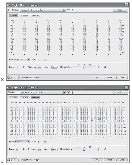
Figure 9.45 (a) Graphic Equalizer with 10 sliders (b) Graphic Equalizer with 30 sliders

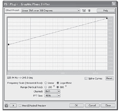
Figure 9.46 Graphic Phase shifter

Notch Filter (Figure 9.47)

This is a specialist effects transform which you will hope never to have to use. It allows you to set up a series of notches in the frequency response to remove discrete frequencies. The Parametric equalizer is shown set to filter 50 Hz and harmonics. This filter comes ready set-up for undertaking just this, the most common disaster recovery task: getting rid of mains hum and buzz resulting from poorly installed equipment (theatre lighting rigs are a common source of buzzes).

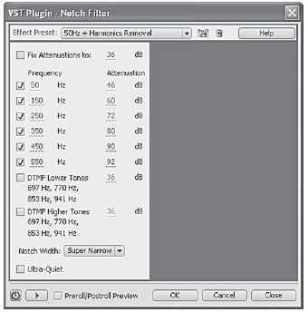
Figure 9.47 Notch filter

In Europe, the frequency of the mains power supply is 50 Hz. In the USA it is 60 Hz. Pure 50 Hz or 60 Hz is a deep bass note. However, mains hum is rarely pure. It comes with harmonics; multiples of the original frequency; 100 Hz, 150 Hz, 200 Hz, etc. (or their equivalents for a 60 Hz original). By ‘notching’ them out, the hope is that they can be removed without affecting the programme material too much. Except in severe cases this works surprisingly well.

The ultra-quiet option throws more processing for an even lower noise figure but Adobe say that you need top quality monitoring to hear the difference, making the processing overhead rarely worthwhile.

The other preset options are to filter DTMF (Dual Tone Multi-Frequency) tones. These are the tones used to ’dial’ telephone numbers. Some commercial radio stations use these to control remote equipment. Apparently they can end up getting mixed with programme material and have to be unscrambled from it. You can do this yourself by using ‘Generate/DTMF tones in Adobe Audition 2.0.

Parametric equalizer (Figure 9.48)

This is another Techie-orientated effects transform. While there is a graphical display like the FFT filter, here the control is applied by putting in figures or by moving sliders. The sliders each side of the graph control the low and high frequencies while the horizontal slider underneath sweep the centre frequencies of five‘middle’ controls. The vertical sliders to the right control the amount of boost or cut for each filter. Most mixers which have middle control usually only have two knobs the ‘±’ control and the frequency sweep. More expensive mixers also have a ‘Q’ knob. This controls the width of the cut or boost. A very high number makes narrow notches a low number makes the boost or cut very wide. Technically ‘Q’ is the ratio of width to centre frequency. Adobe Audition 2.0’s Parametric equalizer also has the option of constant bandwidth as measured in Hertz wherever you are in the frequency range. Like the notch filter it also has an ‘ultra-quiet’ option.

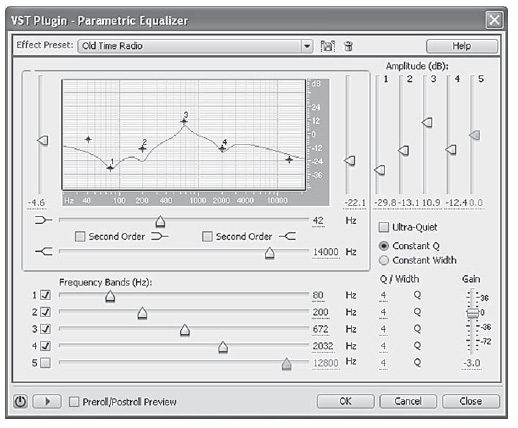
Figure 9.48 Parametric equalizer

Quick filter (Figure 9.49)

In many ways this is a little like another graphic equalizer except that the way it does things is slightly different. Its major difference is that it is two equalizers and implements a transition between the two settings. This can be useful to match different takes where not enough care has been taken to get them consistent in the first place.

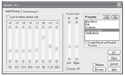
Figure 9.49 Quick filter

It is also potentially useful for drama scene movements. An orchestra in the next room will sound muffled and then, as the characters move into that room, the high frequencies appear. This would have to be done in two stages with the Quick filter locked to apply the ‘other room’ treatment up to the point of the transition. It is then unlocked and the change made over a short section, butted onto the end of the treatment just applied.

However, I strongly recommend not doing it this way but to make a new track with the ‘other room’ treatment on it and use the multitrack editor to manage the change instead (see Transitions on Page 76).

Scientific filters (Figure 9.50)

This is another build-your-own filter kit. Analog filters are effectively made of building blocks, each of which can only change the frequency response by a maximum of 6dB per octave. So, if you need something sharper, then an 18 dB per octave filter needs three building blocks. This sort of filter is known as a third-order filter.

In the analog domain, these filters are built from large quantities of separate components. Each of these components will have manufacturing tolerances of 10 per cent, 5 per cent, 2 per cent or 1 per cent, depending on how much the designer is prepared to pay. This means that anything more than a third- or fourth-order filter is either horrendously expensive or impossible to make, because of the component tolerances blurring everything.

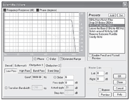
Figure 9.50 Scientific filters

In the digital domain, these components exist as mathematical constructs. They have no manufacturing errors and therefore are exactly the right value. This means that a digital filter can have as many orders as you like, limited only by the resolution of the precision of the internal mathematics used.

Even so you cannot get something for nothing. Heavy filtering will do things to the audio other than change its frequency response. Differential delays will be introduced along with relative phase changes. Some frequencies will tend to ring. Leaving the jargon aside, what this means is that you may achieve the filtering effect that you want, but with the penalty of the result sounding foul.

The Scientific Filter Effects transform offers a set of standard filter options from the engineering canon. The graph shows not only the frequency response, but also the phase or delay penalties. In the end your ears will have to be the judge. If you have a tame audio engineer to hand – assuming that you are not one yourself – then you may persuade them to design you some useful filters optimized for your requirements and saved as presets.

A neat trick to eliminate phase shifts can be to create a batch file which runs the filter you want, then reverses the files and runs the filter again – effectively backwards. It then reverses the file back to normal. The idea is that the shifts cancel themselves out. It also means that you can use a 9th order filter twice rather than an 18th order once.

Plug-ins

Again VST and DirectX plug-ins can be downloaded often with specialist applications.

9.9 Restoration

‘Digitally Remastered’ is a label that is often to be seen on reissued recordings. Adobe Audition 2.0 has a suite of restoration tools that allow you to do this to your own collection of recordings. The filters and EQ we have already examined are part of the armoury but the core is noise reduction software applied to noise from recordings ranging from tape hiss to clicks and plops.

In the world of analog recording, noise reduction refers to the various techniques, mainly associated with the name of Dr Ray Dolby, that reduce the noise inherent in the recording medium. In our digital world, such techniques are not needed except in some data reduction systems such as the NICAM system used for UK television stereo sound. Noise reduction techniques can also be used to reduce natural noise from the environment, such as air conditioning or even distant traffic rumble.

Be warned that this is not magic; there will always be artefacts in the process. A decision always has to be made whether there is an overall improvement. Be very careful when you first use noise reduction techniques as they are very seductive. It takes a little while to sensitize yourself to the artefacts and it is very easy to ‘overcook’ the treatment. As you would expect, the more noise you try to remove, the more you are prone to nasties in the background.

The most common noise reduction side-effect is a reduction of the apparent reverberation time as the bottom of Reverb tails are lost with the noise. In critical cases, it can be best to add, well chosen, artificial Reverb at very low level, to fill in these tails. Getting a good match between the original and the artificial requires good ears.

The basic method of noise reduction is very simple. You find a short section (about 1 second) of audio that is pure noise, in a pause, or the lead into the programme material. This is analysed and used by the program to build up a filter and level guide. Individual bands of frequencies are analysed in the rest of the recording and, when any frequency falls below its threshold in the, what is sometimes known as fingerprint, then this is reduced in level by the set amount. The quieter the noise floor the more effective this is.

However, trying to reduce high wide band hiss levels can leave you with audio suitable only for a science fiction effect. The availability of NR should not be used as an excuse for sloppiness in acquisition of recordings. Don't neglect obtaining the very best quality original recording in the first place.

The classic example of this is old 78rpm recordings. These used a much wider groove. Theoretically, you could use an LP gramophone at 33 rpm to dub a 78 and then speed correct, and noise reduce, in the computer. This would sound foul. Played with the correct equipment, with purpose-designed cartridges and correct sized stylus at the correct playing weight, the quality from a 78 can be astonishing. Remember that most of them were ‘direct-cut’; they were created direct from the output of the live performance mixer. There was no intervening tape stage. Old Mono LPs had wider grooves than stereo records and a wider stylus will produce better outcomes. A turntable equipped with an elliptical stylus will produce the best results from both mono and stereo LPs.

The most effective noise reduction can be achieved just by cleaning the record. Even playing the record through, before dubbing, can clean out a lot of dirt from the groove.

A really bad pressing, with very heavy crackles, will sometimes benefit from wet playing. Literally, pour a layer of distilled water over the playing surface and play it while still wet. This can improve less noisy LPs as well, but once an LP has been wet played, it usually sounds worse once dry again and needs always to be wet played. If it is not your record, then the owner may have an opinion on this!

The subject of gramophone records reminds us of the other major form of noise reduction, namely de-clicking. There are a wide number of different specialist programs that do this, as well as general noise reduction. They vary in how good they are, and how fast they are. If you are likely to be doing a lot of noise reduction then it may be worth your while to invest in one of these specialist programs. Some of these plug-ins can cost more than the program that they plug into!

Click/Pop eliminator (Figure 9.51)

While Adobe Audition 2.0’s de-clicker is not as fast as some, it is very effective and has improved with each revision of the program. You can correct an entire selection or instantly remove a single click if one is highlighted at a high zoom level. You can use the Spectral View feature with the spectral resolution set to 256 bands and a Window Width of 40 per cent to see the clicks in a waveform. You can access these settings in the Display tab of the Preferences dialog box. Clicks will ordinarily be visible as bright vertical bars that go all the way from the top to the bottom of the display. Unfortunately Auditions click eliminators do not have a ‘Keep Clicks’ option which can be very helpful to enable you to increase the threshold until you start to hear distorted programme material and then back off a bit. To satisfy yourself that only clicks rather than music were removed you can save a copy of the original file somewhere, then Mix Paste it (overlap it) over the corrected audio with a setting of 100 per cent and Invert enabled (Figure 9.52).

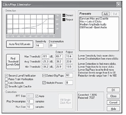
Figure 9.51 Click/pop eliminator

It may take a little trial and error to find the right settings, but the results are well worth it – much better than searching for and replacing each click individually. The parameters that make the most difference in determining how many clicks are repaired are the Detection and Rejection thresholds (the latter of which requires Second Level Verification). Making adjustments to these will have the greatest effects; you might try settings from 10 for a lot of correction, 50 for very little correction on the detection threshold, or 5 to 40 on the rejection threshold.

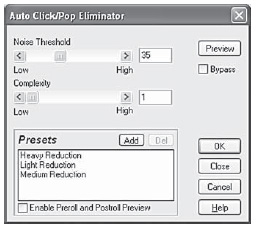
Figure 9.52 Auto Click eliminator

‘Second level verification’ slows the process but enables Adobe Audition 2.0 to distinguish clicks from sharp starting transients in the music. The next parameter that affects the output most is the Run Size. A setting of about 25 is best for high-quality work. If you have the time, running at least three passes will improve the output even more. Each successive pass will be faster than the previous one. ‘Auto Click/Pop eliminator’ provides the same processing quality as the Click/Pop Eliminator effect, but it offers simplified controls and a preview not available with the main version because of its multipass options, etc.

The ‘Fill Single Click Now’ is a particularly powerful option for clicks and plops that resist automatic deletion. If Auto is selected next to FFT Size, then an appropriate FFT size is used for the restoration based on the size of the area being restored. Otherwise, settings of 128 to 256 work very well for filling in single clicks. Once a single click is filled, press the F3 key to repeat the action. You can also create a quick key in the Favorites menu for filling in single click. If the ‘Fill Single Click’ Now button is unavailable, the selected audio range is too long. Click Cancel, and select a shorter range in the waveform display.

Clickfix (Figure 9.53)

If you do a lot of gramophone record transfer then there is an inexpensive commercial de-clicker add-on specifically for Audition written by Jeffery Klein available from http://www.jdklein.com/clickfix/. It uses a proprietary statistical technique to locate clicks and pops. It does not employ edge detection or spectral analysis. He claims that his special technique results in much faster, more accurate click and pop detection than other methods. It is certainly very fast. It does have a ‘Keep only clicks’ option so you can preview the de-clicking and adjust the threshold just short of the breakthrough of programme material. The auto setting covers nearly all my needs for most records.

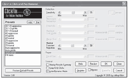
Figure 9.53 Clickfix

Clip Restoration (Figure 9.54)

If your audio is overloaded, you ‘run out of numbers’ and the effect is to clip the peaks, giving them flat tops. You'll hear this as distortion which can be very unpleasant. With this transform, Adobe Audition 2.0 has a fist at restoring the audio. It will never be perfect as data is missing. It does it in two stages. The first is to attenuate the file ‘to make room’ for the restored peaks. It then goes through the file trying to work out what those peaks might have been. How successful this is depends a great deal on the programme material and the extent of clipping but it can make the difference between a usable file and one that has to be junked. (Figures 9.54-9.56)

‘Input Attenuation’ Specifies the amount of amplification that occurs before processing.

‘Overhead’ Specifies the percentage of variation in clipped regions. A value of 0 per cent detects clipping only in perfectly horizontal lines at maximum amplitude. A value of 1 per cent detects clipping beginning at 1 per cent below maximum amplitude. (A value of 1 per cent detects almost all clipping and leads to a more thorough repair.)

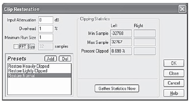
Figure 9.54 Clip restoration

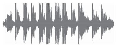
Figure 9.55 Clipped waveform before processing

‘Minimum Run Size’ Specifies the length of the shortest run of clipped samples to repair. A value of 1 repairs all samples that seem to be clipped, while a value of 2 repairs a clipped sample only if it's followed or preceded by another clipped sample.

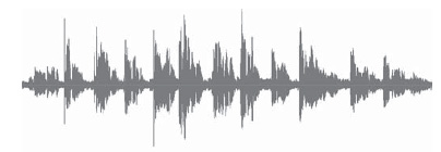
Figure 9.56 Clipped waveform after processing

‘FFT Size’ Sets an FFT Size, measured in samples, if audio is severely clipped (e.g., because of too much bass). In this case, you want to estimate the higher frequency signals in the clipped areas. Using the FFT Size option in other situations might help with some types of clipping. (Try a setting of 40 for normal clipped audio.) In general, however, leave FFT Size unselected as then Adobe Audition uses spline curve estimation.

‘Clipping Statistics’ Shows the minimum and maximum sample values found in the current selected range, as well as the per cent of samples clipped based on that data.

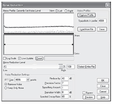
Figure 9.57 Noise Reduction

‘Gather Statistics Now’ Updates the Clipping Statistics values for the current selection or file.

To retain amplitude when restoring clipped audio, work at 32-bit resolution for more precise editing. Then apply the Clip Restoration effect with no attenuation, followed by the Hard Limiting effect with a Boost value of 0 and a Limit value of -0.2dB (Figure 9.57).

Noise Reduction options

‘View’ displays either the left or right channel noise profile. The amount of noise reduction is always the same for both channels. To perform separate levels of reduction on each channel, edit the channels individually.

Noise Profile graph represents, in yellow, the amount of noise reduction that will occur at any particular frequency. Adjust the graph by moving the Noise Reduction Level slider.

‘Capture Profile’ extracts a noise profile from a selected range, indicating only background noise. Adobe Audition gathers statistical information about the background noise so it can remove it from the remainder of the waveform.

If the selected range is too short, Capture Profile is disabled. Reduce the FFT Size or select a longer range of noise. If you can't find a longer range, copy and paste the currently selected range to create one. (You can later remove the pasted noise by using the Edit > Delete Selection command.)

‘Snapshots In Profile’ determines how many snapshots of noise to include in the captured profile. A value of 4000 is optimal for producing accurate data.

Very small values greatly affect the quality of the various noise reduction levels. With more samples, a noise reduction level of 100 will likely cut out more noise, but also cut out more original signal. However, a low noise reduction level with more samples will also cut out more noise, but likely will not disrupt the intended signal.

‘Load From File’ opens any noise profile previously saved from Adobe Audition in FFT format. However, you can apply noise profiles only to identical sample types. (e.g., you can't apply a 22 kHz, mono, 16-bit profile to 44 kHz, stereo, 8-bit samples.)

‘Save’ saves the noise profile as an .FFT file, which contains information about sample type, FFT size and three sets of FFT coefficients: one for the lowest amount of noise found, one for the highest amount and one for the power average.

‘Select Entire File’ lets you apply a previously captured noise reduction profile to the entire file.

Reduction graph sets the amount of noise reduction at certain frequency ranges. For example, if you need noise reduction only in the higher frequencies, adjust the chart to give less noise reduction in the low frequencies, or alternatively, more reduction in the higher frequencies.

The graph depicts frequency along the x-axis (horizontal) and the amount of noise reduction along the y-axis (vertical). If the graph is flattened (click Reset), then the amount of noise reduction used is based on the noise profile exactly. The readout below the graph displays the frequency and adjustment percentage at the position of the cursor.

Select Log Scale to divide the graph evenly into 10 octaves.

Deselect Log Scale to divide the graph linearly, with each 1000 kHz (for example) taking up the same amount of horizontal width.

‘Live Update’ enables the Noise Profile graph to be redrawn as you move control points on the Reduction graph.

‘Noise Reduction Level’ adjusts the amount of noise reduction to be applied to the waveform or selection. Alternatively, enter the desired amount in the text box to the right of the slider.

Sometimes the remaining audio will have a flanged or phase-like quality. For better results, undo the effect and try a lower setting.

‘FFT Size’ determines how many individual frequency bands are analysed. This option causes the most drastic changes in quality. The noise in each frequency band is treated separately, so the more bands you have, the finer frequency detail you get in removing noise. For example, if there's a 120 Hz hum, but not many frequency bands, frequencies from 80 Hz on up to 160 Hz may be affected. With more bands, less spacing between them occurs, so the actual noise is detected and removed more precisely. However, with too many bands, time slurring occurs, making the resulting sound reverberant or echo-like (with pre- and post-echoes). So the trade-off is frequency resolution versus time resolution, with lower FFT sizes giving better time resolution and higher FFT sizes giving better frequency resolution. Good settings for FFT Size range from 4096 to 12000.

‘Remove Noise, Keep Only Noise’ removes noise or removes all audio except for noise.

‘Reduce By’ determines the level of noise reduction. Values between 6 and 30 dB work well. To reduce bubbly background effects, enter lower values.

‘Precision Factor’ affects distortions in amplitude. Values of 5 and up work best, and odd numbers are best for symmetric properties. With values of 3 or less, the FFT is performed in giant blocks and a drop or spike in volume can occur at the intervals between blocks. Values beyond 10 cause no noticeable change in quality, but they increase the processing time.

‘Smoothing Amount’ takes into account the standard deviation, or variance, of the noise signal at each band. Bands that vary greatly when analysed (such as white noise) will be smoothed differently than constant bands (like a 60 cycle hum). In general, increasing the smoothing amount (up to 2 or so) reduces burbly background artefacts at the expense of raising the overall background broadband noise level.

‘Transition Width’ determines the range between what is noise and what remains. For example, a transition width of zero applies a sharp, noise gate-type curve to each frequency band. If the audio in the band is just above the threshold, it remains; if it's just below, it's truncated to silence. Conversely, you can specify a range over which the audio fades to silence based upon the input level. For example, if the transition width is 10 dB, and the cut-off point (scanned noise level for the particular band) is -60 dB, then audio at -60 dB stays the same, audio at -62 dB is reduced (to about -64 dB) and so on, and audio at -70 dB is removed entirely. Again, if the width is zero, then audio just below -60 dB is removed entirely, while audio just above it remains untouched. Negative widths go above the cut-off point, so in the preceding example, a width of -10dB creates a range from -60 to -50 dB.

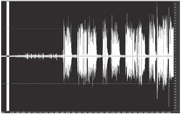
Figure 9.58 Selecting noise at start of track

‘Spectral Decay Rate’ specifies the percentage of frequencies processed when audio falls below the noise floor. Fine-tuning this percentage allows greater noise reduction with fewer artefacts. Values of 40 to 75 per cent work best. Below those values, bubbly-sounding artefacts are often heard; above those values, excessive noise typically remains.

Figure 9.58 shows the beginning of the vocal track from a cassette-based four-track machine with its dbx noise reduction switched off. Looking closely at the track you can see that some of the noise is from tape hiss and hum, but there is also spill from the vocalist's headphones. I have selected a couple of seconds where there is no spill, only machine noise. If we take a noise print we can see that it has picked up the hum on the output of the four- track machine and raises the threshold at the hum frequencies (Figure 9.59).

Figure 9.59 Noise profile showing hum

Having taken the noise print, we return to Adobe Audition 2.0 and select the whole wave and initiate the noise reduction process. In Figure 9.60, you can clearly see that it has removed the hiss and hum but left the headphone spill. It will depend on the material whether this amount of noise reduction sounds acceptable. The spill can be removed selectively using the Effects/mute menu option.

9.10 Special effects

Convolution (Figure 9.61)

Convolution is the effect of multiplying every sample in one wave or impulse by the samples that are contained within another waveform. In a sense, this feature uses one waveform to ‘model’ the sound of another waveform. The result can be that of filtering, echoing, phase shifting or any combination of these effects. That is, any filtered version of a waveform can be echoed at any delay, any number of times. For example, ‘convolving’ someone saying ‘Hey’ with a drum track (short full spectrum sounds such as snares work best) will result in the drums saying ‘Hey’ each time they are hit. You can build impulses from scratch by specifying how to filter the audio and the delay at which it should be echoed, or by copying audio directly from a waveform.

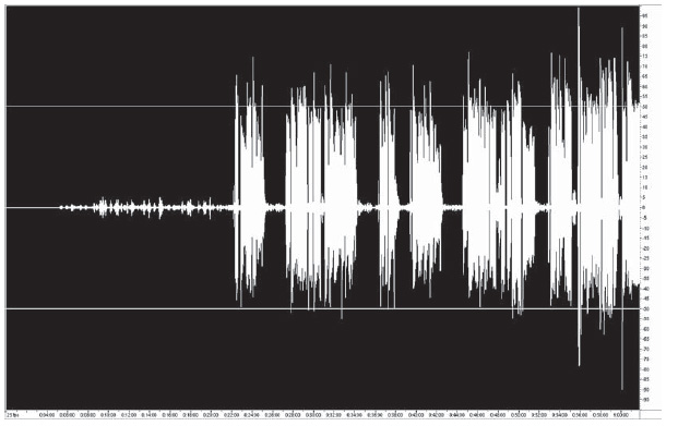
Figure 9.60 Hiss and hum removed but headphone spill still visible

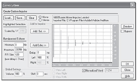
Figure 9.61 Convolution Dialog

To get a feel for Convolution, load up and play with some of the sample Impulse files (.IMP) that were installed with Adobe Audition 2.0. You can find them in the /IMPS directory inside of the directory where you have installed Adobe Audition 2.0.

With the proper impulses, any reverberant space can be simulated. For example, if you have an impulse of your favourite cathedral, and convolute it with any mono audio (left and right channels the same) then the result would sound as if that audio were played in that cathedral. You can generate an impulse like this by going to the cathedral in question, standing in the spot where you would like the audio to appear it is coming from, and generating a loud impulsive noise, like a ‘snap’ or loud ‘click’. You can make a stereo recording of this ‘click’ from any location within the cathedral. If you used this recording as an impulse, then convolution with it will sound as if the listener were in the exact position of the recording equipment, and the audio being convoluted were at the location of the ‘click’. Most of Adobe Audition 2.0’s Reverb transforms are based on convolution algorithms.

Another interesting use for convolution is to generate an infinite sustained sound of anything. For example, one singing ‘aaaaaah’ for 1 second could be turned into thousands of people singing ‘aaaaaah’ for any length of time by using some dynamically expanded white noise (which sounds a lot like radio static).

To send any portion of unprocessed ‘dry’ signal back out, simply add a full spectrum echo at 0 millisecond. The Left and Right volume percentages will be the resulting volume of the dry signal in the left and right channels.

Distortion (Figure 9.62)

We spend most of our time trying to avoid distortion but there are times when we want it. This can be for dramatic purposes or for things like a ‘fuzz’ guitar. This transform does this by ‘remapping’ samples to different values.

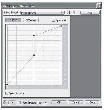
Figure 9.62 Distortion

9.11 Time/pitch

Adobe Audition 2.0 has five effects transforms to do with pitch changing and time stretching.

The first creates Doppler shifts (Figure 9.63). Doppler shifts are the pitch changes you hear when a noise making object passes you. As it approaches the pitch is increased and then once it passes the pitch is reduced compared with what its pitch is when stationary. Perhaps, the most common time we hear this is when an emergency services vehicle speed by sounding its siren. This transform allows you to take a static recording of, say, a siren and process it so that it sounds as though it is moving. The volume can be handled as well if you want. The transform can handle circular movement like a merry-go-round as well.

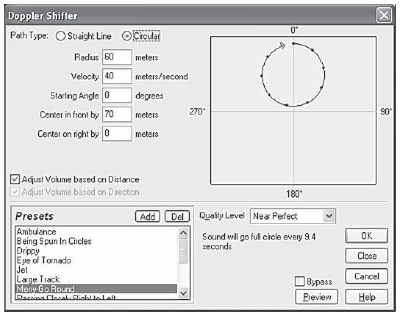
Figure 9.63 Doppler shifter

The second time/pitch transform is the pitch bender (Figure 9.64). This is the direct equivalent of varying the speed of a recording tape. It can handle a fixed change, or make a transition from one ‘speed’ to another. You can draw the curve as to how it does this. As such it forms the ideal basis to repair a recording made on an analog machine with failing batteries.

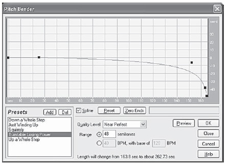
Figure 9.64 Pitch Bender

What happens when the tape speed varies on an analog tape is that, as the speed decreases, so the pitch decreases. If the tape is running at half speed, everything takes twice as long and the pitch is 1 octave lower. However, with computer manipulation this relationship no longer need be maintained.

Adobe Audition 2.0’s next effects transform is Pitch correction (Figure 9.65). This can be a boon if your vocal talent is not that talented.

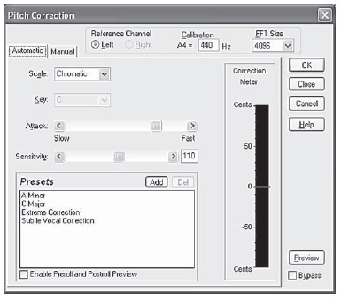
Figure 9.65 Pitch correction

The Time/Pitch > Pitch Correction effect provides two ways to adjust the pitch adjustments of vocals or solo instruments. Automatic mode analyses the audio content and automatically corrects the pitch based on the key you define, without making you analyse each note. Manual mode creates a pitch profile that you can adjust note-by-note. You can even overcorrect vocals to create robotic-sounding effects.

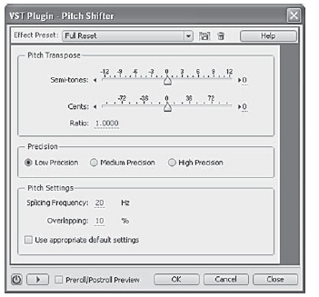
Figure 9.66 Pitch shifter

The Pitch Correction effect detects the pitch of the source audio and measures the periodic cycle of the waveform to determine its pitch. The effect is most effective with audio that contains a periodic signal (i.e. audio with one note at a time, such as saxophone, violin or vocal parts). Nonperiodic audio, or any audio with a high noise floor, can disrupt the effect's ability to detect the incoming pitch, resulting in incomplete pitch correction (Figure 9.66).

The Pitch shifter allows you to change the overall speed of a recording without changing the pitch or, alternatively, change the pitch without changing the speed.

This is not done by magic, but by manipulation of the audio. Indeed there were analog devices that did the same, just not very well. Even in the digital domain you are less likely to get good results with extreme settings.

Pitch manipulation is a specialized form of delay and works because, as in the chorus effect, changing a delay while listening to a sound changes its pitch while the delay is being changed. As soon as the delay stops being changed, the original pitch is restored whatever the final delay. Anyone who has varispeeded a tape recorder while it was recording and listened to its output will know the temporary pitch change effect lasts only while the speed is changing. It returns to normal the moment a new speed is stabilized.

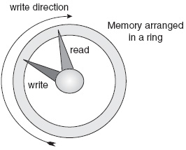
Figure 9.67 Digital delay and pitch change

A digital delay circuit can be thought of as memory arranged in a ring, as in Figure 9.67. One pointer rotates round the ring, writing the audio data. A second pointer rotates round the same ring, reading the data. The separation between the two represents the delay between the input and output. In a simple delay, this separation is adjusted to obtain the required delay.

In a pitch changer, the pointers ‘rotate’ at different speeds. If the read pointer is faster than the write pointer, then the pitch is raised. If the read pointer travels slower than the write pointer then the pitch is lowered.

Quite obviously, there is a problem each time the pointers ‘cross over’ when a ‘glitch’ occurs. The skill of the software writer is to write processing software that disguises this. The software either creates, or loses, data to sustain the differently pitched audio output.

Uses

•  Time stretching: A radio commercial lasting 31 seconds can be reduced to 30 seconds by speeding it up by the required amount while maintaining the original pitch.

•  Singers, with insufficient breath control, can be made to appear to be singing long, sustained notes by slowing down the recording and pitch changing to the original.

•  Pitch changing: The pitch change can be useful for correcting singers who are out of tune.

•  Voice disguise: These devices are sometimes used to disguise voices in radio and television news programmes. There was also a fashion for them to be used for alien voices in science fiction programmes.

•  Music: With judicious use of feedback, pitch changing can be used to thicken and enrich sounds.

9.12 Spatial effects

By spatial effects, we usually mean effects where the sound appears to be coming from somewhere other than between the speakers. A general atmosphere seems to fill the room, or a spaceship flies overhead, from behind you.

Techniques like Dolby stereo use extra loudspeakers, and special processing, to get their directional effect. DVD recordings can use five channels of audio to move sounds, but simple stereo can be beefed up, with a little simple manipulation.

Normally we think of stereo consisting of left and right channels. The relative volume of these channels controls where a sound comes from. A more sophisticated way of thinking about stereo is as an MS signal, MS standing for ‘middle’ and ‘side’ NOT mono and stereo. The middle signal consists of a simple mix of the left and right signals in phase. The side signal is again a simple mix of the left and right signals with the right channel phase reversed (inverted).

The middle signal is what is used as the mono signal in broadcasting. If you feed your stereo channel with a simple mono signal panned to the centre – say a presenter's voice – then there will be no side signal; the left and right channels are identical and, because the right-hand signal is inverted, they cancel themselves out.

As the mono signal is panned to one side the side signal increases until the sound is panned fully to one side. At this point, the middle and side signals are equal in level. Once you are thinking in this way, you can consider what happens when you increase the side signal so that it is larger than the middle signal. Doing this can pan the sound image outside the speakers. How effective this will be depends on the programme material. As the out-of-phase level is increased, the image will soon collapse and appear to come from inside the head.

With a really complex stereo signal, tweaking the side level can give dramatic dimensional effects. It is also a means of creating a fake stereo signal from a mono original.

Faking stereo

You sometimes need to fake a stereo sound from a mono source. This can range from a unique background sound to a period train, only ever recorded in mono, passing across the sound stage between the speakers.

There are several techniques open to the balancer. With continuous sounds such as applause, trains, atmospheres, etc., it is often possible to get a spread effect by playing two copies of the same (or different) sources. One is panned left and the other panned right with, perhaps, a third in the centre. If they get into close synchronization then compatibility problems may arise with phasing on a mono radio receiver. In Adobe Audition 2.0, this is easily done by using duplicate copies on different tracks and sliding the tracks relative to each other to get the right effect.

A better way, which gives no compatibility problems, is to play one source in mono and the other phase-reversed so that it only contributes to the stereo signal. This bonus sound is not heard by the mono listener as it cancels out.

Again duplicate tracks are used except that one (not both) of the duplicate tracks is converted to a stereo wave file and one channel (say the right) is phase-reversed (inverted). For a discrete sound, like an aircraft taking off or a train passing, sliding this track to delay the sound by 50 to 100 milliseconds can produce good results, especially if the volume envelope on this difference channel is manipulated.

If you want a directional sound, like a train passing between the speakers, you need to do this in two stages. First generate a ‘spread’ train and mix this down to create a new stereo wave file. This can then be panned using the pan envelope control.

With atmospheres, very long delays can be used – try 30 seconds (if the FX is long enough). Changing the level of the out-of-phase signal in sympathy with the sound can improve realism.

Thunder claps can be particularly effective, if you run different mono claps on the inphase and out-of-phase tracks. It can be difficult to find genuine stereo thunder that rolls around the room as effectively.

The same techniques can be used to beef up stereo sounds which do not come up to your expectations. Provided the sound is OK for any mono listener – if the recording is to be broadcast – then anything you add out of phase to your mix will be a bonus to the stereo sound without affecting the mono. If you can guarantee your recording will never be heard in mono then compatibility is not a problem. Remember that, in addition to mono radios, there are mono cassette players.

9.13 Basic effects

There are three basic effects at the top of the Effect menu drop down. Although they are very simple they are extremely useful.

Invert

The Invert menu option is a fairly specialized effects transform. All it does is to invert the waveform so that positive becomes negative and negative becomes positive.

In music balancing, this is the equivalent of the phase reverse switch on a mixing console. You can find, when you come to a mix down, that a microphone was out of phase with others used at the same time.

Microphones should be in phase. This means that their output voltages are going in the same direction; an impulse that makes the diaphragm move inwards on the microphones produces the same direction voltage. All the microphones should produce a positive voltage, or all the microphones should produce a negative voltage. It doesn't matter which, as long as they are the same. If they are out of phase, they tend to cancel, and the mix can sound a bit like a drainpipe.

The left and right channels of stereo should be in phase too as, otherwise, a central image seems to be coming from inside the head, rather than from between the speakers. Worse, if the recording is broadcast, people listening on mono receivers will not hear anything in the centre as it will cancel out. See description of Adobe Audition 2.0’s Phase Analysis on Page 164 for more information.

Reverse

Reverse does just literally that; it reverses the sound so that the beginning becomes the end. Its main uses are for producing reversed echo and alien voices. It can also be used in batch files to reduce phase shift errors using filters by running the filter, reversing the audio, running the filter again so that any phase timing errors are reversed and then reverse the audio back to normal again.

Reversed echo is often used for magical effects: witches and aliens. It sometimes has a role in music, although it is an entirely unnatural effect.

A multistage process is used. First the programme material is reversed. Then it has a reverberation effects transform applied to it. That transformed recording is then reversed again. This restores the original speech, etc. to the right way round, but with the Reverb now reversed. What was a Reverb die-away now becomes a build up. Satisfyingly weird effects can be created this way. However, the relative balance is critical so, again, it is best if the reversed Reverb is created as a ‘wet-only’ track, so that it can be mixed with the original while you can actually hear the intended effect.

If you have a performer who is a good mimic, you can create a really good alien voice by getting them to record the lines and then reversing them. The performer now imitates the sound of the reversed speech – this takes some practice. He, or she, is then recorded imitating the backwards speech and then that recording itself is reversed. All being well, an inhuman voice will be heard speaking very strangely but intelligibly. This sort of trick has to be done in relatively short takes to work well.

Mute

This mutes the selected section of the wave file. Its main purpose is for music balancing, as you can use it to remove spill, coughs and sneezes from, say, a vocal track. This means that you do not have to set the volume envelope for each vocal entry and exit, but can guarantee absolute digital silence in breaks in the performance.

Don't confuse this with Generate/silence. The difference between the two is that this trans-form mutes a section of existing audio, making no change to its length. Generate/silence inserts a given number of seconds of silence at the cursor so that inserting 10 seconds of silence will make the file 10 seconds longer.

Generate silence, DTMF, noise and tones are discussed in Chapter 11 ‘Mastering’.

9.14 Multitrack effects

The Multitrack view of Adobe Audition 2.0 has three effects transforms of its own. They are here because they generate a new track or tracks in the multitrack view.

The envelope follower and the vocoder combine, non-destructively, two different audio tracks to create a third. It can be very frustrating to try to use these as the menu options are grayed out unless the conditions are right. To use Adobe Audition 2.0’s vocoder or envelope follower, you have to both select two tracks and highlight the section to be processed. The easiest way to do this is to have the control and process tracks adjacent to each other and to highlight both with one action. Place the mouse cursor over the first track, press and hold down the left mouse button at the beginning of, or just before, the wanted section and drag the cursor down to the next track and along to the end of the section required. You can do this starting from the end and moving to the beginning if you prefer. This is often the best way if you are starting at the very beginning (0:00.00). Both tracks will now be highlighted and the Effects/vocoder and Effects/Envelope follower menu options will be enabled (this happens only if two tracks are selected).

If the two tracks are not adjacent, you can still do the same, except that the tracks in between will also be enabled. You need individually to deselect these by holding the Control key down and single clicking on each.

Selecting the section and then enabling two tracks by holding the control key down and single clicking on them will also work.

Envelope follower (Figure 9.68)

The Envelope follower varies the output level of one waveform, based on the input level of the other. The amplitude map, or envelope, of one waveform (the analysis wave) is applied to the material of a second waveform (the process wave), which results in the second waveform taking on the amplitude characteristics of the first waveform. This lets you, for example, have a bass guitar line which only sounds when a drum is being hit. In this example you would have the drum waveform as the analysis wave, and the bass guitar waveform as the process wave.

The dialog has a go at guessing which way round the tracks should be but often gets this wrong. You can switch them by clicking on the drop-downs at the top of the dialog. Once you have found a setting that works you can save it as a preset.

When you click OK the normal progress dialog will appear and a new track will appear. Normally the next available one will be used but you can change it with the ‘Output to’ drop down.

Frequency Band Splitter

The frequency band splitter takes the output of a single track and creates up to 9 new tracks each with a different frequency band of audio. This presents intriguing possibilities as you can separately treat these bands with any of the processing available to Adobe Audition 2.0. At the simplest, you could boost the level of a cymbal to change the sound or you could even compress it. By putting compression on each track you have the basis of a multiband compressor for mastering. This is one of those tools which, while appearing simple opens up a host of possibilities.

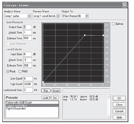
Figure 9.68 Envelope follower

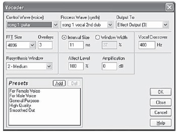
Figure 9.69 Frequency Band Splitter

You can have up to 9 bands and you can change the crossover frequencies by typing them in the left hand boxes. The number of tracks produced is selected by the buttons at the side, These are not toggles but clicking one will produce that number of bands (Figure 9.69).

Vocoder (Figure 9.70)

A vocoder is a special effect which can make inanimate objects appear to speak or sing. If you want the leaves of a tree to talk or sing, then the vocoder may do what you want. It takes one sound (the process signal) and modulates it with the second (the control signal). Modulate a telephone bell with someone saying ‘ring ring’ and you could have a talking telephone bell.

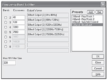
Figure 9.70 Vocoder

The top three boxes tell you about the two input tracks and where the transform will be placed. The left and centre drop-downs allow you to set which track is the control wave and which is the process file. The third box displays the next track empty at the selected area where the resulting transform will be placed.

Some presets are provided and the help file advises ‘For ease of use, set Window Width to about 90 per cent, use 3 or 4 overlays, set Resynthesis Window to 1 or 2, and choose an FFT size between 2048 and 6400.’ A fair amount of fiddling must be expected to get good results.

9.15 Real-time controls and effects

In the multitrack editor you have various controls in the left hand column. Which ones you see are controlled by the icons at the top (Figure 9.71 – see Chapter 7 ‘Multitrack’).

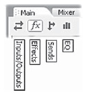
Figure 9.71 Facility view selector icons

Most of the non-process effects that were described earlier in the Wave Editor view are also available as real-time effects within the multitrack editor. But beware! Effects are very processor intensive and you will need as fast a computer as possible. If you have a slower machine you may find that you will only be able to use a small number at a time and will, having rehearsed the setting to get them how you like them within a mix, then process the actual wave file to reduce processing load when playing the multitrack mix.

In an ideal world all your FX should be in real time just like on an ordinary sound mixer. This is because everything interacts. A vocal line that sounded fine may need hardening if you have made the backing music brighter.

On the other hand the ability to pre-record your effects does allow you to use the slow computer you have now rather than having to save up for something faster before you can do anything.

A useful compromise, especially for Reverb is not to alter the original wave file but to generate a new wave file which is just the Reverb for a track. Controlling the level of this additional track requires much less processing power.

Adobe Audition 2.0 has a neat halfway house. You can lock or ‘freeze’ the effects once you have a setting that you like. There will then be a pause while the progress bar shows it processing and saving the FX. It can be left untouched and the processing overhead will be small but a click of a button will restore the track to real-time effects (Figure 9.72).

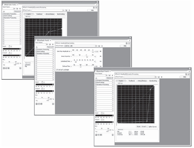
Figure 9.72 Single channel Effects rack containing three effects. Each effect is selectable for viewing. Shown is a vocal track with soft compression, followed by hard limiting and then gating to remove spill.

Track Equalizer

Each track comes with its own real-time parametric equalizer. If you have clicked the EQ icon at the top of the column you see the basic settings in numerical form (Figure 9.73).

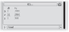
Figure 9.73 Numerical track equalizer view

Clicking the EQ button will reveal a graphical display so that you literally can see, as well as hear, what you are doing. (Figure 9.74)

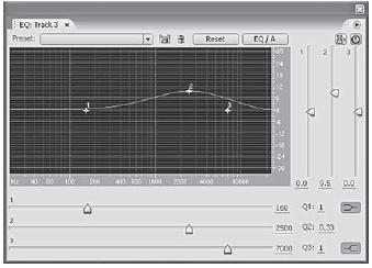
Figure 9.74

In fact there are two alternative equalizers, ‘A’ and ‘B’ which can be switched between easily by single clicking the ‘EQ’ button. It will toggle between showing ‘EQ/A’ or ‘EQ/B’. At its simplest, this allows you to use ‘EQ/B’ as a flat reference to switch the EQ in and out. Of course, you can also use it to switch between alternative EQs but you can achieve this by using the power button which toggles from green and white. Sometimes you need the alternative EQ to be an ‘equalized flat’. For example, you may already established that you need a high-pass filter setting on the low control but now want to try a bit of middle boost on top of that. You used to be able to copy a setting from one EQ to another by double-clicking in the ‘EQ’ button but this has not been continued in version 2.0. However presets can be created in one and used in another.

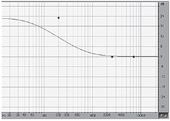
Figure 9.75

The low and high controls can be switched between shelf and Band EQ. (Figures 9.75 and 9.76)

Shelf EQ operates like an ordinary bass or treble control on a Hi-Fi. Unlike an ordinary Hi-Fi, you can alter where the ‘turnover’ from flat to sloping takes place. The boost out cut levels out after a couple of octaves so as not to excessively boost extreme high or low frequencies.

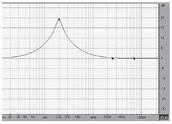
Figure 9.76

Clicking the button toggles the filter into a band type equalizer that operates like a middle control. Thus you can have three middle controls which can be much more useful than shelf EQ. Shelf is indicated by the Q value turning black.

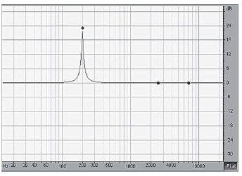
Figure 9.77 Middle control high Q setting

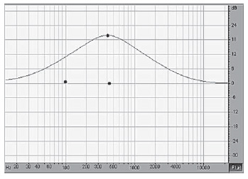
Figure 9.78 Middle control low Q setting

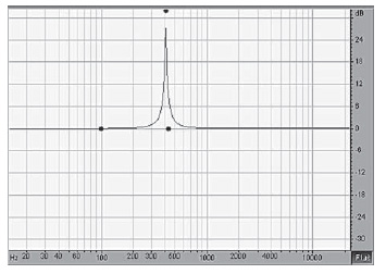
Figure 9.79 Maximum boost to isolate unwanted frequency.

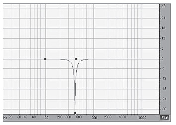
Figure 9.80 Maximum cut to remove unwanted frequency

The middle is, as you would expect always set to Band. Any of the bands can be adjusted for Q. Any of the controls can always be controlled for the active frequency they start operating.

Semi-professional mixers sometimes have just a simple plus or minus control for the middle. Better ones have a sweep control where you can adjust the frequency of boost or cut. The very best also have a ‘Q’ control that adjust the width of the boost or cut. The very narrow setting can be useful for removing interference sound that have been picked up ranging from buzzes to lighting whistles (Figures 9.77-9.80).

(But don't forget the notch filter is already set up to reduce mains electricity related buzzes).

A good technique to remove a single frequency is to set the band control to maximum Q, the narrowest setting, at maximum boost. move the frequency control until the unwanted sound is found and has become much louder. Now move the level control from maximum boost to maximum cut and the unwanted frequency should be tamed or eliminated. In practice, you may find that a maximum setting will affect the overall wanted sound as well as removing the unwanted. Here, a compromise has to be made. Only your ears can tell you how much.

If you are not using a track equalizer, make sure that its ‘power’ button is off so as not to use unnecessary processor power.