
“Well, I think if you say you’re going to do something and don’t do it, that’s trustworthiness.” | ||
| --George W. Bush, in a CNN online chat, August 30, 2000 | ||
In previous chapters, we have defined fuzzing, exposed fuzzing targets, enumerated various fuzzing classes, and discussed various methods of data generation. However, we have yet to cover the matter of tracking the progress of our various fuzzer technologies. The notion of fuzzer tracking has not yet received a great deal of attention in the security community. To our knowledge, none of the currently available commercial or freely available fuzzers have addressed this topic.
In this chapter we define fuzzer tracking, also known as code coverage. We discuss its benefits, explore various implementation approaches, and, of course, in the spirit of the rest of this book, build a functional prototype that can be united with our previously developed fuzzers to provide a more powerful level of analysis.
At the lowest programmatic level, the CPU is executing assembly instructions, or commands that the CPU understands. The available instruction set will differ depending on the underlying architecture of your target. The familiar IA-32 / x86 architecture for example, is a Complex Instruction Set Computer[1] (CISC) architecture that exposes more than 500 instructions, including, of course, the ability to perform basic mathematic operations and manipulate memory. Contrast this architecture with a Reduced Instruction Set Computer (RISC) microprocessor, such as SPARC, which exposes fewer than 200 instructions.[2]
Whether you are working on CISC or RISC, the actual individual instructions are less often written by a human programmer but rather compiled or translated into this low-level language from a higher level language, such as C or C++. In general, the programs you interact with on a regular basis contain from tens of thousands to millions of instructions. Every interaction with the software causes instruction execution. The simple acts of clicking your mouse, processing of a network request, or opening a file all require numerous instructions to be executed.
If we are able to cause a Voice over IP (VoIP) software phone (softphone) to crash during a fuzz audit, how do we know which set of instructions was responsible for the fault? The typical approach taken by researchers today is to work backward, by examining logs and attaching a debugger to pinpoint the location of the fault. An alternative approach is to work forward, by actively monitoring which instructions are executed in response to our generated fuzz requests. Some debuggers, such as OllyDbg, implement tracing functionality that allows users to track all executed instructions. Unfortunately, such tracing functionality is typically very resource intensive and not practical beyond very focused efforts. Following our example, when the VoIP softphone does crash, we can review the executed instructions to determine where along the process the fault occurred.
When writing software, one of the most basic forms of debugging it is to insert print statements throughout code. This way, as the program executes, the developer is made aware of where execution is taking place and the order in which the various logical blocks are executing. We essentially want to accomplish the same task but at a lower level where we don’t have the ability to insert arbitrary print statements.
We define this process of monitoring and recording the exact instructions executed during the processing of various requests as “fuzzer tracking.” A more generic term for this process with which you might already be familiar is code coverage, and this term will be used interchangeably throughout the chapter. Fuzzer tracking is a fairly simple process and as we will soon see, creates a number of opportunities for us to improve our fuzz analysis.
An essential concept with regard to our discussion on code coverage is the understanding of binary visualization, which will be utilized in the design and development of our prototype fuzzer tracker. Disassembled binaries can be visualized as graphs known as call graphs. This is accomplished by representing each function as a node and the calls between functions as edges between the nodes. This is a useful abstraction for viewing the structure of an overall binary as well as the relationships between the various functions. Consider the contrived example in Figure 23.1.
Most of the nodes in Figure 23.1 contain a label prefixed with sub_ followed by an eight- character hexadecimal number representing the address of the subroutine in memory. This naming convention is used by the DataRescue Interactive Disassembler Pro (IDA Pro)[4] disassembler for automatically generating names for functions without symbolic information. Other disassembling engines use similar naming schemes. When analyzing closed source binary applications, the lack of symbolic information results in the majority of functions being named in this form. Two of the nodes in Figure 23.1 do have symbolic names and were labeled appropriately, snprintf() and recv(). From a quick glance at this call graph, we can immediately determine that the unnamed subroutines sub_00000110() and sub_00000330(), are responsible for processing network data due to their relationship to recv().
Disassembled functions can also be visualized as graphs known as CFGs. This is accomplished by representing each basic block as a node and the branches between the basic blocks as edges between the nodes. This naturally leads to the question of what a basic block is? A basic block is defined as a sequence of instructions where each instruction within the block is guaranteed to be run, in order, once the first instruction of the basic block is reached. To elaborate further, a basic block typically starts at the following conditions:
The start of a function
The target of a branch instruction
The instruction after a branch instruction
Basic blocks typically terminate at the following conditions:
A branch instruction
A return instruction
This is a simplified list of basic block start and stop points. A more complete list would take into consideration calls to functions that do not return and exception handling. However, for our purposes, this definition will do just fine.
To drive the point home, consider the following excerpt of instructions from an imaginary subroutine sub_00000010. The [el] sequences in Figure 23.2 represent any number of arbitrary nonbranching instructions. This view of a disassembled function is also known as a dead listing, an example of which is shown in Figure 23.2.
Breaking the dead listing into basic blocks is a simple task following the previously outlined rules. The first basic block starts at the top of the function at 0x00000010 and ends with the first branch instruction at 0x00000025. The next instruction after the branch at 0x0000002B, as well as the target of the branch at 0x00000050, each mark the start of a new basic block. Once broken into its basic blocks, the CFG of the subroutine shown in Figure 23.2 looks like Figure 23.3.
This is a useful abstraction for viewing the various control-flow paths through a function as well as spotting logical loops. The key point to remember with CFGs is that each block of instructions is guaranteed to be executed together. In other words, if the first instruction in the block is executed, then all the instructions in that block will be executed. Later, we will see how this knowledge can help us take necessary shortcuts in the development of our fuzzer tracker.
We can take a number of approaches to implementing a custom code coverage tool. If you have already read prior chapters, perhaps the first approach that comes to mind is to use a debugger with tracing functionality to monitor and log every instruction that is executed. This is the exact approach that OllyDbg utilizes to implement its “debug race into” and “debug race over” functionality. We could replicate this functionality by building on the same PyDbg library we utilized in Chapter 20, “In-Memory Fuzzing: Automation,” with the following logic:
This simplistic approach can be implemented on top of PyDbg in just under 50 lines of Python. However, it is not a favorable approach as instrumentation of each instruction within a process via a debugger adds a great deal of latency that, in many cases, makes the approach unusable. If you don’t believe it, try it out for yourself with the relevant code listed in the sidebar, which is also available online at http://www.fuzzing.org. Furthermore, simply determining and logging executed instructions covers only a single aspect of our overall goal. To produce better reports we need more information about our target.
We implement our fuzzer tracker using a three-phase approach:
First, we will statically profile our target.
The second step is the actual live tracking and recording of which instructions within our target are executing in response to our fuzzer.
The third and final step involves cross-referencing the generated live data with the profile data from Step 1 to produce a useful tracking report.
Assuming we have the capability of determining which instructions were executed within any given application, what other bits of information would we like to know about that application to make more sense of the data set at hand? For example, we minimally would like to know the total number of instructions in our target. That way, we can determine what percentage of the underlying code within a target application is responsible for handling any given task. Ideally, we would like to have a more detailed breakdown of the instruction set:
How many instructions are in our target?
How many functions?
How many basic blocks?
Which instructions within our target pertain to standard support libraries?
Which instructions within our target did our developers write?
What lines of source does any individual instruction translate from?
What instructions and data are reachable and can be influenced by network or file data?
Various tools and techniques can be utilized to answer these questions. Most development environments have the capability of producing symbolic debugger information that can assist us in more accurately addressing these questions as well. For our purposes, we assume that access to source code is not readily available.
To provide answers to these key questions, we build our profiler on top of IDA Pro’s disassembler. We can easily glean statistics on instructions and functions from IDA. By implementing a simple algorithm based on the rules for basic blocks, we can easily extract a list of all the basic blocks contained within each function as well.
Because single stepping through a program can be time consuming and unnecessary, how else can we trace instruction coverage? Recall from our previous definition that a basic block is simply a sequence of instructions where each instruction within the block is guaranteed to be run, in order. If we can track the execution of basic blocks, then we are inherently tracking the execution of instructions. We can accomplish this task with the combination of a debugger and information gleaned from our profiling step. Utilizing the PyDbg library, we can implement this concept with the following logic:
By recording hits on basic blocks as opposed to individual instructions, we can greatly improve performance over traditional tracing functionality, such as the limited approach utilized by OllyDbg mentioned earlier. If we are only interested in which basic blocks are executed, then there is no need to restore breakpoints in Step 4. Once a basic block is hit, we will have recorded this fact within the handler and we are no longer interested in knowing if and when the basic block is ever reached again in the future. However, if we are also interested in the sequence in which basic blocks are executed, we must restore breakpoints in Step 4. If the same basic block is hit again and again, perhaps within a loop, then we will have recorded each iterative hit. Restoring breakpoints provides us with more contextual information. Letting breakpoints expire gives us a boost in speed. The decision to take one approach versus the other will likely depend on the task at hand and as such should be configurable as an option in our tool.
In situations where we are tracking a large number of basic blocks, the tracking speed might not be where we want it to be. In such situations, we can further abstract from the instruction level by tracking executed functions versus executed basic blocks. This requires minimal changes to our logic. Simply set breakpoints on the basic blocks that start a function instead of on all basic blocks. Again, the decision to take one approach versus the other might change from run to run and as such should be a configurable option in our tool.
Another convenient feature to implement in our fuzzer tracking tool is the ability to filter prerecorded code coverage from new recordings. This feature can be leveraged to easily filter out the functions, basic blocks, and instructions that are responsible for processing tasks in which we are not interested. An example of such uninteresting code is that which is responsible for processing GUI events (mouse clicks, menu selection, etc.). We’ll see how this can come into play later in a sidebar on code coverage for vulnerability discovery.
In the third and final step, we combine the information from static profiling with the outputs from our runtime tracker to produce accurate and useful reports addressing points such as these:
What areas of code are responsible for processing our inputs?
What percentage of our target have we covered?
What was the execution path that resulted in a particular fault?
Which logical decisions within our target were not exercised?
Which logical decisions within our target are dependent directly on supplied data?
The last two bullet points in this list pertain to making educated decisions on ways to improve our fuzzer, rather than pinpointing any specific flaw in that actual target application. We cover these points further later in the chapter when discussing the various benefits that fuzzer tracking can provide us.
Code Coverage for Vulnerability Discovery
A remotely exploitable buffer overflow affecting Microsoft Outlook Express during the parsing of Network News Transfer Protocol (NNTP) responses[5] was published on June 14, 2005. Let’s examine the benefits of code coverage analysis on this issue as it applies to a vulnerability researcher. The crux of the Microsoft advisory reads as follows:
A remote code execution vulnerability exists in Outlook Express when it is used as a newsgroup reader. An attacker could exploit the vulnerability by constructing a malicious newsgroup server that could that potentially allow remote code execution if a user queried the server for news. An attacker who successfully exploited this vulnerability could take complete control of an affected system. However, user interaction is required to exploit this vulnerability.
Not much information to go on there, and certainly not enough to be of any use to IDS or IPS signature developers, for example. All we know is that the bug manifests itself when connecting Outlook Express to a malicious NNTP server. Utilizing a previously available and open source code coverage tool, Process Stalker,[6] let’s try and see if we can narrow down the issue some. The specific command-line options and usage of Process Stalker are outside the scope of this book. To see the specific details behind this example, please see the original OpenRCE article.[7]
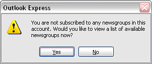
By installing the available patch and monitoring which files within the Outlook Express installation directory were modified, we are able to determine that MSOE.DLL must contain the vulnerable code. Analyzing this module with the Process Stalker IDA Pro plug-in reveals a total of approximately 4,800 functions and 58,000 basic blocks. It would be quite a daunting task to manually sift through this data. To narrow our field of interest, we can utilize Process Stalker to locate the code paths associated with having Outlook Express connect to an arbitrary NNTP server. Although this is certainly effective in reducing the analysis space, we can do better. Recall from a previous statement that every interaction with our target in turn results in instruction execution. In the current situation, this means that when we access a malicious NNTP server through the ‘news://’ URI handler in Internet Explorer, for example, our code coverage tool will unnecessarily record the code responsible for starting Outlook Express, the code responsible for painting on-screen items such as windows and dialog boxes, and the code responsible for processing user-driven GUI events such as clicking buttons. For example, when connecting to an NNTP server for the first time, the dialog box shown in Figure 23.4 is presented.
The creation, handling, and tearing down of this dialog box are far from interesting for our purposes. To further narrow our analysis scope, we can use Process Stalker to record only the code responsible for handling various GUI tasks. We do this by attaching to and interacting with Outlook Express without actually connecting to an NNTP server. Next, we remove the overlapping coverage between our GUI-only and server-connect recordings to pinpoint specifically the code responsible for parsing the NNTP server request. When all is said and done, we are able to reduce our field of view to 91 functions. Of the 1,337 (we swear this number was not made up) basic blocks across those 91 functions, only 747 were actually visited in the server-connect recording. Compared with the 58,000 that we began with, this is a significant and helpful reduction!
Applying a simple script to locate the basic blocks responsible for moving server-supplied data around further reduces the number to a meager 26 basic blocks, the second of which reveals the exact specifics of the vulnerability: An arbitrary amount of server-supplied data, delimited by spaces, is copied into a static 16-byte stack buffer. Wonderful, we can now whip up the exploit ... er ... vulnerability protection filter and get back home in time for the latest episode of The Sopranos.[8]
The PyDbg library, which we previously worked with, is in fact a subcomponent of a larger reverse engineering framework, named PaiMei. PaiMei is an actively developed, open source Python reverse engineering framework freely available for download.[9] PaiMei can essentially be thought of as a reverse engineer’s Swiss army knife and can be of assistance in various advanced fuzzing tasks, such as intelligent exception detection and processing, a topic we cover in depth in Chapter 24, “Intelligent Fault Detection.” There already exists a code coverage tool bundled with the framework named PAIMEIpstalker (also called Process Stalker or PStalker). Although the tool might not produce the exact reports you want out of the box, as the framework and bundled applications are open source they can be modified to meet whatever your specific needs are for a given project. The framework breaks down into the following core components:
PyDbg. A pure Python win32 debugging abstraction class.
pGRAPH. A graph abstraction layer with separate classes for nodes, edges, and clusters.
PIDA. Built on top of pGRAPH, PIDA aims to provide an abstract and persistent interface over binaries (DLLs and EXEs) with separate classes for representing functions, basic blocks, and instructions. The end result is the creation of a portable file, that, when loaded, allows you to arbitrarily navigate throughout the entire original binary.
We are already familiar with the interface to PyDbg from earlier. Scripting on top of PIDA is even simpler. The PIDA interface allows us to navigate a binary as a graph of graphs, enumerating nodes as function or basic blocks and the edges between them. Consider the following example:
import pida

module = pida.load("target.exe.pida")

# step through each function in the module.
for func module.functions.values():
    print "%08x - %s" % (func.ea_start, func.name)

    # step through each basic block in the function.
    for bb in func.basic_blocks.values():
        print "	%08x" % bb.ea_start

        # step through each instruction in the
        # basic block.
        for ins in bb.instructions.values():
            print "		%08x %s" % (ins.ea, ins.disasm)
We begin in this snippet by loading a previously analyzed and saved PIDA file as a module in the script. Next we step through each function in the module, printing the starting address and symbolic name along the way. We next step through each basic block contained within the current function. For each basic block, we continue further by stepping through the contained instructions and printing the instruction address and disassembly along the way. Based on our previous outline, it might already be obvious to you how we can combine PyDbg and PIDA to easily prototype a basic block-level code coverage tool. A layer above the core components, you will find the remainder of the PaiMei framework broken into the following overarching components:
Utilities. A set of utilities for accomplishing various repetitive tasks. There is a specific utility class we are interested in,
process_stalker.py, which was written to provide an abstracted interface to code coverage functionality.Console. A pluggable WxPython application for quickly and efficiently creating custom GUI interfaces to newly created tools. This is how we interface with the pstalker code coverage module.
Scripts. Individual scripts for accomplishing various tasks, one very important example of which is the
pida_dump.pyIDA Python script, which is run from IDA Pro to generate .PIDA files.
The pstalker code coverage tool is interfaced through the aforementioned WxPython GUI and as we will soon see, relies on a number of the components exposed by the PaiMei framework. After exploring the various subcomponents of this code coverage tool, we examine its usage by way of a case study.
The PStalker module is one of many modules available for use under the PaiMei graphical console. In the PStalker initial screen displayed in Figure 23.5, you can see that the interface is broken into three distinct columns.
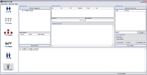
The Data Sources column exposes the functionality necessary for creating and managing the targets to be stalked as well as loading the appropriate PIDA modules. The Data Exploration column is where the results of any individual code coverage run or stalk. Finally, the Data Capture column is where runtime configuration options and the target executable are specified. The general workflow associated with this tool is as follows (read on for specifics):
Create a new target, tag, or both. Targets can contain multiple tags and each individual tag contains its own saved code coverage data.
Select a tag for stalking.
Load PIDA modules for every .DLL and the .EXE code for which coverage information is required.
Launch the target process.
Refresh the process list under the data capture panel and select the target process for attaching or browse to the target process for loading.
Configure the code coverage options and attach to the selected target.
Interact with the target while code coverage is being recorded.
When appropriate, detach from the target and wait for PStalker to export captured items to the database.
Load the recorded hits to begin exploring recorded data.
The online documentation[10] for PaiMei includes a full-length video demonstrating the use of the PStalker module. If you haven’t ever seen it before, now is a good time to check it out prior to continuing.
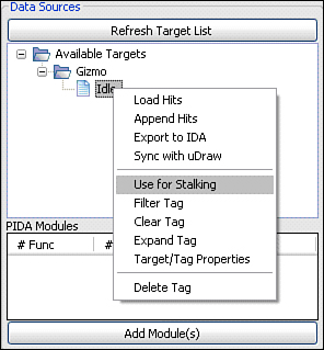
Once consolewide MySQL connectivity is established through the Connections menu, select the Retrieve Target List button to propagate the data source explorer tree. This list will be empty the first time the application is run. New targets can be created from the context menu of the root node labeled Available Targets. Use the context menu for individual targets to delete the individual target, add a tag under the target, and load the hits from all tags under the target into the data exploration pane. The context menu for individual tags exposes a number of features:
Load hits. Clear the data exploration pane and load the hits associated with the selected tag.
Append hits. Append the hits associated with the selected tag after any existing data currently in the exploration pane.
Export to IDA. Export the hits under the selected tag as an IDC script suitable for import in IDA to highlight the hit functions and blocks.
Sync with uDraw. Synchronize the data exploration pane on the consolewide uDraw connection. Dual monitors are very helpful for this feature.
Use for stalking. Store all recorded hits during data capture phase to the selected tag. A tag must be selected for stalking prior to attaching to a process.
Filter tag. Do not record hits for any of the nodes or basic blocks under the selected tag in future stalks. More than one tag can be marked for filtering.
Clear tag. Keep the tag but remove all the hits stored under the tag. PStalker cannot stalk into a tag with any preexisting data. To overwrite the contents of a tag it must be cleared first.
Expand tag. For each hit function in the tag, generate and add an entry for every contained basic block, even if that basic block was not explicitly hit.
Target/tag properties. Modify the tag name, view or edit tag notes, or modify the target name.
Delete tag. Remove the tag and all the hits stored under the tag.
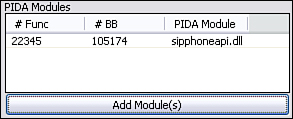
The PIDA modules list control displays the list of loaded PIDA modules as well their individual function and basic block counts. Prior to attaching to the target process, at least one PIDA module must be loaded. During the code coverage phase, the PIDA module is referenced for setting breakpoints on functions or basic blocks. A PIDA module can be removed from the list through a context menu.
The data exploration pane is broken into three sections. The first section is propagated when hits are loaded or appended from the Data Sources column. Each hit is displayed in a scrollable list box. Selecting one of the line items displays, if available, the context data associated with that hit in the Dereferenced Data text control. In between the list and text controls, there are two progress bars that represent the total code coverage based on the number of individually hit basic blocks and functions listed in the exploration pane against the number of total basic blocks and functions across all loaded PIDA modules.
Once a tag has been selected for stalking, the selected filters have been applied, and the target PIDA modules have loaded, the next step is to actually attach to and stalk the target process.
Click the Retrieve List button to display an up-to-date process list, with newer processes listed at the bottom. Select the target process for attaching or browse to the target process for loading and select the desired coverage depth. Select Functions to monitor and track which functions are executed within the target process or select Basic Blocks to further scrutinize the individual basic blocks executed.
The Restore BPs check box controls whether or not to restore breakpoints after they have been hit. To determine what code was executed within the target, leave the option disabled. Alternatively, to determine both what was executed and the order in which it was executed, this option should be enabled.
The Heavy check box controls whether or not PStalker will save context data at each recorded hit. Disable this option for increased speed. Clear the Unhandled Only check box to receive notification of debug exception events even if the debuggee is capable of correctly handling them.
Finally, with all options set and the target process selected, click the Attach and Start Tracking button to begin code coverage. Watch the log window for runtime information.
There is one main limitation to this tool of which you should be aware. Specifically, the tool is reliant on the static analysis of the target binaries as provided by DataRescue’s IDA Pro; therefore, the tool will fail when IDA Pro makes mistakes. For example, if data is misrepresented as code, bad things can happen when PStalker sets breakpoints on that data. This is the most common reason for failure. Disabling the Make final pass analysis kernel option in IDA Pro prior to the autoanalysis will disable the aggressive logic that makes these types of errors. However, the overall analysis will also suffer. Furthermore, packed or self-modifying code cannot currently be traced.
The typical user will not likely need to know how data is organized and stored behind the scenes of the PStalker code coverage tool. Such users can take advantage of the abstraction provided by the tool and utilize it as is. More detailed knowledge of the database schema will, however, be required in the event that the need to build custom extensions or reporting arises. As such, this section is dedicated to dissecting the behind-the-scenes data storage mechanism.
All of the target and code coverage data is stored in a MySQL database server. The information is stored across three tables: cc_hits, cc_tags, and cc_targets. As shown in the following SQL table structure, the cc_targets database contains a simple list of target names, an automatically generated unique numeric identifier, and a text field for storing any pertinent notes related to the target:
CREATE TABLE  'paimei'.'cc_targets' (
  'id' int(10) unsigned NOT NULL auto_increment,
  'target' varchar(255) NOT NULL default '',
  'notes' text NOT NULL,
  PRIMARY KEY  ('id')
) ENGINE=MyISAM;
The next SQL table structure is of the cc_tags database, which contains an automatically generated unique numeric identifier, the identifier of the target the tag is associated with, the name of the tag, and once again a text field for storing any pertinent notes regarding the tag.
CREATE TABLE  'paimei'.'cc_tags' (
  'id' int(10) unsigned NOT NULL auto_increment,
  'target_id' int(10) unsigned NOT NULL default '0',
  'tag' varchar(255) NOT NULL default '',
  'notes' text NOT NULL,
  PRIMARY KEY  ('id')
) ENGINE=MyISAM;
Finally, as shown in the following SQL table structure, the cc_hits database contains the bulk of the recorded runtime code coverage information:
CREATE TABLE  'paimei'.'cc_hits' (
  'target_id' int(10) unsigned NOT NULL default '0',
  'tag_id' int(10) unsigned NOT NULL default '0',
  'num' int(10) unsigned NOT NULL default '0',
  'timestamp' int(10) unsigned NOT NULL default '0',
  'eip' int(10) unsigned NOT NULL default '0',
  'tid' int(10) unsigned NOT NULL default '0',
  'eax' int(10) unsigned NOT NULL default '0',
  'ebx' int(10) unsigned NOT NULL default '0',
  'ecx' int(10) unsigned NOT NULL default '0',
  'edx' int(10) unsigned NOT NULL default '0',
  'edi' int(10) unsigned NOT NULL default '0',
  'esi' int(10) unsigned NOT NULL default '0',
  'ebp' int(10) unsigned NOT NULL default '0',
  'esp' int(10) unsigned NOT NULL default '0',
  'esp_4' int(10) unsigned NOT NULL default '0',
  'esp_8' int(10) unsigned NOT NULL default '0',
  'esp_c' int(10) unsigned NOT NULL default '0',
  'esp_10' int(10) unsigned NOT NULL default '0',
  'eax_deref' text NOT NULL,
  'ebx_deref' text NOT NULL,
  'ecx_deref' text NOT NULL,
  'edx_deref' text NOT NULL,
  'edi_deref' text NOT NULL,
  'esi_deref' text NOT NULL,
  'ebp_deref' text NOT NULL,
  'esp_deref' text NOT NULL,
  'esp_4_deref' text NOT NULL,
  'esp_8_deref' text NOT NULL,
  'esp_c_deref' text NOT NULL,
  'esp_10_deref' text NOT NULL,
  'is_function' int(1) unsigned NOT NULL default '0',
  'module' varchar(255) NOT NULL default '',
  'base' int(10) unsigned NOT NULL default '0',
  PRIMARY KEY  ('target_id','tag_id','num'),
  KEY 'tag_id' ('tag_id'),
  KEY 'target_id' ('target_id')
) ENGINE=MyISAM;
The fields from the cc_hits table break down as follows:
target_id & tag_id. These two fields tie any individual row within this table to a specific target and tag combination.
num. This field holds the numeric order in which the code block represented by the individual row was executed within the specified target–tag combination.
timestamp. This stores the number of seconds since the UNIX Epoch (January 1 1970, 00:00:00 GMT), a format easily converted to other representations.
eip. This field stores the absolute address of the executed code block that the individual row represents; this field is commonly formatted as a hexadecimal number.
tid. This field stores the identifier of the thread responsible for executing the block of code at eip. The thread identifier is assigned by the Windows OS and is stored to differentiate between the code blocks executed by various threads in a multithreaded application.
eax, ebx, ecx, edx, edi, esi, ebp, and esp. These fields contain the numeric values for each of the eight general-purpose registers at the time of execution. For each of the general-purpose registers and stored stack offsets a deref field exists, containing the ASCII data behind the specific register as a pointer. At the end of the ASCII data string is a tag, which is one of (stack), (heap) or (global), representing where the dereferenced data was found. The moniker N/A is used in cases where dereferencing is not possible as the relevant register did not contain a dereferenceable address.
esp_4, esp_8, esp_c, and esp_10: These fields contain the numeric values at their relevant stack offsets (esp_4 = [esp+4], esp_8 = [esp+8], etc.).
is_function. This is a boolean field where a value of 1 denotes that the hit data block (at eip) is the start of a function.
module. This field stores the name of the module in which the hit occurred.
base. This field contains the numerical base address of the module specified in the previous field. This information can be used in conjunction with eip to calculate the offset within the module that the hit data block occurred at.
The open data storage provides advanced users with an outlet for generating custom and more advanced reports beyond what the PStalker tool provides by default. Let’s put the tracker to the test with a full-fledged case study.
For a practical case study, we will apply the PStalker code coverage tool to determine the relative completeness of a fuzz audit. Our target software is the Gizmo Project,[11] a VoIP, instant messaging (IM), and telephony communication suite. Figure 23.6 is a commented screen shot from the Gizmo Project Web site detailing the major features of the tool.
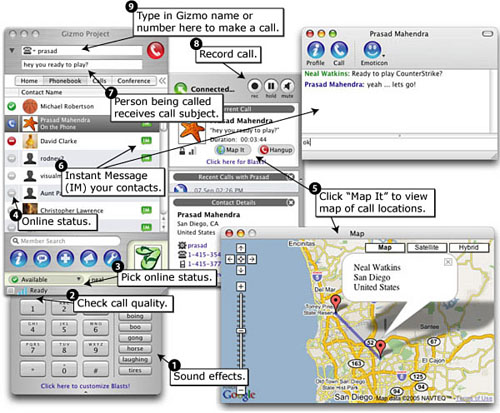
Gizmo implements an impressive number of features that are among the reasons for its soaring popularity. Seen by many as a possible Skype[12] “killer,” Gizmo differentiates itself from the ubiquitous Skype by building on open VoIP standards such as the Session Initiation Protocol (SIP - RFC 3261), as opposed to implementing a closed proprietary system. This decision allows Gizmo to interoperate with other SIP compatible solutions. This decision also allows us to test Gizmo with standard VoIP security testing tools. Now that the crosshairs are set on the target software, we must next pick the target protocol and select an appropriate fuzzer.
We will be testing Gizmo’s ability to handle malformed SIP packets. Although there are a few VoIP protocols we could target, SIP is a good choice as most VoIP telephony begins with a signaling negotiation through this protocol. There are also already a few free SIP fuzzers available. For our test, we will be using a freely available SIP fuzzer distributed by the University of Oulu Department of Electrical and Information Engineering named PROTOS Test-Suite: c07-sip.[13] The PROTOS test suite contains 4,527 individual test cases distributed in a single Java JAR file. Although the test suite is limited to testing only INVITE messages, it is perfectly suitable for our needs. A partial motivation for choosing this fuzzer is that the team responsible for its development has spun off a commercial version through the company Codenomicon.[14] The commercial version of the SIP test suite explores the SIP protocol in greater depth and bundles 31,971 individual test cases.
Our goal is as follows: Utilize PStalker while running through the complete set of PROTOS test cases to measure the exercised code coverage. This case study can be expanded on to accomplish practical tasks such as comparing fuzzing solutions or determining the confidence of a given audit. The individual benefits of utilizing code coverage as a metric are further discussed later in the chapter.
The PROTOS test suite runs from the command line and exposes nearly 20 options for tweaking its runtime behavior, shown here from the output of the help switch:
$ java -jar c07-sip-r2.jar -h

Usage java -jar <jarfile>.jar [ [OPTIONS] | -touri <SIP-URI> ]
  -touri  <addr>        Recipient of the request
                        Example: <addr> : [email protected]
  -fromuri <addr>       Initiator of the request
                        Default: [email protected]
  -sendto <domain>      Send packets to <domain> instead of
                        domainname of -touri
  -callid <callid>      Call id to start test-case call ids from
                        Default: 0
  -dport <port>         Portnumber to send packets on host.
                        Default: 5060
  -lport <port>         Local portnumber to send packets from
                        Default: 5060
  -delay <ms>           Time to wait before sending new test-case
                        Defaults to 100 ms (milliseconds)
  -replywait <ms>       Maximum time to wait for host to reply
                        Defaults to 100 ms (milliseconds)
  -file <file>          Send file <file> instead of test-case(s)
  -help                 Display this help
  -jarfile <file>       Get data from an alternate bugcat
                        JAR-file <file>
  -showreply            Show received packets
  -showsent             Show sent packets
  -teardown             Send CANCEL/ACK
  -single <index>       Inject a single test-case <index>
  -start <index>        Inject test-cases starting from <index>
  -stop <index>         Stop test-case injection to <index>
  -maxpdusize <int>     Maximum PDU size
                        Default to 65507 bytes
  -validcase            Send valid case (case #0) after each
                        test-case and wait for a response. May
                        be used to check if the target is still
                        responding. Default: off
Your mileage might vary, but we found the following options to work best (where the touri option is the only mandatory one):
java -jar c07-sip-r2.jar -touri [email protected]
                         -teardown
                         -sendto 10.20.30.40
                         -dport 64064
                         -delay 2000
                         -validcase
The delay option of two seconds gives Gizmo some time to free resources, update its GUI, and otherwise recover between test cases. The validcase parameter specifies that PROTOS should ensure that a valid communication is capable of transpiring after each test case, prior to continuing. This rudimentary technique allows the fuzzer to detect when something has gone awry with the target and cease testing. In our situation this is an important factor because Gizmo does actually crash! Fortunately for Gizmo, the vulnerability is triggered due to a null-pointer dereference and is therefore not exploitable. Nonetheless, the issue exists (Hint: It occurs within the first 250 test cases). Download the test suite and find out for yourself.
[*] 0x004fd5d6 mov eax,[esi+0x38] from thread 196 caused access violation when
attempting to read from 0x00000038
CONTEXT DUMP
EIP: 004fd5d6 mov eax,[esi+0x38]
EAX: 0419fdfc ( 68812284) -> <CCallMgr::IgnoreCall() (stack)
EBX: 006ca788 ( 7120776) -> e(elllllllllllllllllllll (PGPlsp.dll.data)
ECX: 00000000 ( 0) -> N/A
EDX: 00be0003 ( 12451843) -> N/A
EDI: 00000000 ( 0) -> N/A
ESI: 00000000 ( 0) -> N/A
EBP: 00000000 ( 0) -> N/A
ESP: 0419fdd8 ( 68812248) -> NR (stack)
+00: 861c524e (2250003022) -> N/A
+04: 0065d7fa ( 6674426) -> N/A
+08: 00000001 ( 1) -> N/A
+0c: 0419fe4c ( 68812364) -> xN (stack)
+10: 0419ff9c ( 68812700) -> raOo|hoho||@ho0@*@b0zp (stack)
+14: 0061cb99 ( 6409113) -> N/A
disasm around:
0x004fd5c7 xor eax,esp
0x004fd5c9 push eax
0x004fd5ca lea eax,[esp+0x24]
0x004fd5ce mov fs:[0x0],eax
0x004fd5d4 mov esi,ecx
0x004fd5d6 mov eax,[esi+0x38]
0x004fd5d9 push eax
0x004fd5da lea eax,[esp+0xc]
0x004fd5de push eax
0x004fd5df call 0x52cc60
0x004fd5e4 add esp,0x8
SEH unwind:
0419ff9c -> 006171e8: mov edx,[esp+0x8]
0419ffdc -> 006172d7: mov edx,[esp+0x8]
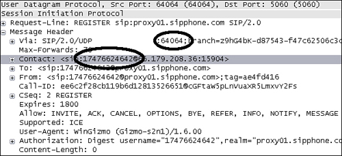
ffffffff -> 7c839aa8: push ebpThe touri and dport parameters were gleaned through examination of packets traveling to or from port 5060 (the standard SIP port) during Gizmo startup. Figure 23.7 shows the relevant excerpt with the interesting values highlighted.
The number 17476624642 is the actual phone number assigned to our Gizmo account and the port 64064 appears to be the standard Gizmo client-side SIP port. Our strategy is in place. The target software, protocol, and fuzzer have been chosen and the options for the fuzzer have been decided on. Now, it’s time to move to the tactical portion of the case study.
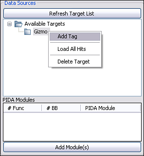
We are fuzzing SIP and are therefore interested specifically in the SIP processing code. Luckily for us, the code is easily isolated, as the library name SIPPhoneAPI.dll immediately stands out as our target. First things first: Load the library into IDA Pro and run the pida_dump.py script to generate SIPPhoneAPI.pida. Because we are only interested in monitoring code coverage, specifying “basic blocks” as the analysis depth for the pida_dump.py script will result in a performance improvement. Next, let’s fire up PaiMei and walk through the necessary prerequisites to get the code coverage operational. For more information regarding specific usage of PaiMei, refer to the online documentation.[15] The first step as depicted in Figure 23.8 is to create a target that we name “Gizmo” and add a tag named “Idle.” We’ll use the “Idle” tag to record the code coverage within Gizmo at “stand still.” This is not a necessary step, but as you can specify multiple tags for recording and furthermore select individual tags for filtering, it never hurts to be as granular as possible. The “Idle” tag must then be selected for “Stalking” as shown in Figure 23.9 and the SIPPhoneAPI PIDA file must be loaded as shown in Figure 23.10.
Once the data sources are set up and a tag is selected, we next select the target process and capture options and begin recording code coverage. Figure 23.11 shows the configured options we will be using. The Refresh Process List button retrieves a list of currently running processes. For our example we choose to attach to a running instance of Gizmo as opposed to loading a new instance from startup.
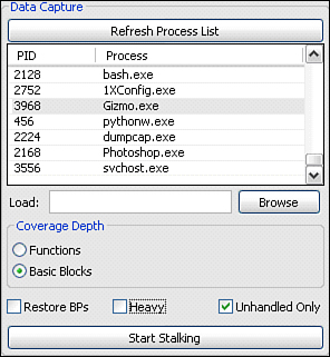
Under Coverage Depth, we select Basic Blocks to get the most granular level of code coverage. As you saw previously from Figure 23.10, our target library has just under 25,000 functions and more than four times that many basic blocks. Therefore, if speed is a concern for us, we can sacrifice granularity for improved performance by alternatively selecting Functions for the coverage depth.
The Restore BPs check box flags whether or not basic blocks should be tracked beyond their first hit. We are only interested where execution has taken us so we can leave this disabled and improve performance.
Finally, we clear the Heavy check box. This check box flags whether or not the code coverage tool should perform runtime context inspection at each breakpoint and save the discovered contents. Again, as we are only interested in code coverage, the additional data is unnecessary so we avoid the performance hit of needlessly capturing it.
Once we click “Start Stalking,” the code coverage tool attaches to Gizmo and begins monitoring execution. If you are interested in the specific details of how the process ensues behind the scenes, refer to the PaiMei documentation. Once activated, log messages indicating the actions and progress of PStalker are written to the log pane. The following example excerpt demonstrates a successful start:
[*] Stalking module sipphoneapi.dll
[*] Loading 0x7c900000 WINDOWSsystem32
tdll.dll
[*] Loading 0x7c800000 WINDOWSsystem32kernel32.dll
[*] Loading 0x76b40000 WINDOWSsystem32winmm.dll
[*] Loading 0x77d40000 WINDOWSsystem32user32.dll
[*] Loading 0x77f10000 WINDOWSsystem32gdi32.dll
[*] Loading 0x77dd0000 WINDOWSsystem32advapi32.dll
[*] Loading 0x77e70000 WINDOWSsystem32
pcrt4.dll
[*] Loading 0x76d60000 WINDOWSsystem32iphlpapi.dll
[*] Loading 0x77c10000 WINDOWSsystem32msvcrt.dll
[*] Loading 0x71ab0000 WINDOWSsystem32ws2_32.dll
[*] Loading 0x71aa0000 WINDOWSsystem32ws2help.dll
[*] Loading 0x10000000 InternetGizmo ProjectSipphoneAPI.dll
[*] Setting 105174 breakpoints on basic blocks in SipphoneAPI.dll
[*] Loading 0x16000000 InternetGizmo Projectdnssd.dll
[*] Loading 0x006f0000 InternetGizmo Projectlibeay32.dll
[*] Loading 0x71ad0000 WINDOWSsystem32wsock32.dll
[*] Loading 0x7c340000 InternetGizmo ProjectMSVCR71.DLL
[*] Loading 0x00340000 InternetGizmo Projectssleay32.dll
[*] Loading 0x774e0000 WINDOWSsystem32ole32.dll
[*] Loading 0x77120000 WINDOWSsystem32oleaut32.dll
[*] Loading 0x00370000 InternetGizmo ProjectIdleHook.dll
[*] Loading 0x61410000 WINDOWSsystem32urlmon.dll
...
[*] debugger hit 10221d31 cc #1
[*] debugger hit 10221d4b cc #2
[*] debugger hit 10221d67 cc #3
[*] debugger hit 10221e20 cc #4
[*] debugger hit 10221e58 cc #5
[*] debugger hit 10221e5c cc #6
[*] debugger hit 10221e6a cc #7
[*] debugger hit 10221e6e cc #8
[*] debugger hit 10221e7e cc #9
[*] debugger hit 10221ea4 cc #10
[*] debugger hit 1028c2d0 cc #11
[*] debugger hit 1028c30d cc #12
[*] debugger hit 1028c369 cc #13
[*] debugger hit 1028c37b cc #14
...
We can now activate the fuzzer and track the code executed during idle time. To continue, we wait for the list of hit breakpoints to taper off indicating that the code within the SIP library that executes while Gizmo sits idly has been exhausted. Next we create a new tag and select it as the active tag through the right-click menu by choosing Use for Stalking. Finally, we right-click the previously created “Idle” tag and choose Filter Tag. This effectively ignores all basic blocks that were executed during the idle state. Now we can start the fuzzer and watch it run. Figure 23.12 shows the code coverage observed in response to all 4,527 PROTOS test cases.
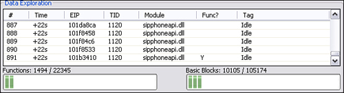
In conclusion, the PROTOS test suite was able to reach only roughly 6 percent of the functions and 9 percent of the basic blocks within the SIPPhoneAPI library. That’s not bad for a free test suite, but it illustrates why running a single test suite is not the equivalent of a comprehensive audit. After running the test suite we have failed to test the majority of the code and it’s unlikely that we’ve comprehensively tested functionality within the code that we did hit. These coverage results can, however, be improved by adding a process restart mechanism in between short intervals of test cases. The reasoning behind this is that even though Gizmo successfully responds to the valid test cases, we instructed PROTOS to insert between malformed tests, Gizmo still ceases to operate correctly after some time and the code coverage suffers. Restarting the process resets internal state and restores full functionality, allowing us to more accurately and thoroughly examine the target.
Considering that PROTOS contains only 1/7 of the test cases of its commercial sister, can we expect seven times more code coverage from the commercial version? Probably not. Although increased code coverage is expected, there is no consistent or predictable ratio between the number of test cases and the resulting amount of code exercised. Only empirical results can be accurate.
So what do we gain from tracking fuzzers in this manner and how can we improve on the technique? The next section provides us with some answers to these questions.
Traditionally, fuzzing has not been conducted in a very scientific manner. Frequently, security researchers and QA engineers hack together rudimentary scripts for generating malformed data, allow their creation to execute for an arbitrary period of time, and call it quits. With the recent rise in commercial fuzzing solutions, you will find shops that take fuzzing one step further toward scientific testing by utilizing an exhaustive list of the test cases developed by a commercial vendor such as Codenomicon. For security researchers simply looking for vulnerabilities to report or sell, there’s often no need to take the process any further. Given the present state of software security, the current methodologies are sufficient for generating an endless laundry list of bugs and vulnerabilities. However, with increasing maturity and awareness of both secure development and testing, the need for a more scientific approach will be desired. Software developers and QA teams concerned with finding all vulnerabilities, not just the low-hanging fruit, will be more concerned with taking a more scientific approach to fuzzing. Fuzzer tracking is a necessary step in this direction.
Keeping with the same example used throughout this chapter, consider the various parties involved in developing the latest VoIP softphone release and the benefits they might realize from fuzzer tracking. For the product manager, knowing the specific areas of tested code allows him to determine more accurately and with more confidence the level of testing to which their product has been subjected. Consider the following statement, for example: “Our latest VoIP softphone release passed 45,000 malicious test cases.” No proof is provided to validate this claim. Perhaps of the 45,000 malicious cases, only 5,000 of them covered features exposed by the target softphone. It is also possible that the entire test set exercised only 10 percent of the available features exposed by the target softphone. Who knows, maybe the test cases were written by really brilliant engineers and covered the entire code base. The latter case would be wonderful, but again, without code coverage analysis there is no way to determine the validity of the original claim. Coupling a fuzzer tracker with the same test set might lead to the following, more informative statement: “Our latest VoIP softphone release passed 45,000 malicious test cases, exhaustively testing over 90 percent of our code base.”
For the QA engineer, determining which areas of the softphone were not tested allows him to create more intelligent test cases for the next round of fuzzing. For example, during fuzzer tracking against the softphone the engineer might have noticed that the test cases generated by the fuzzer consistently trigger a routine named parse_sip(). Drilling down into that routine he observes that although the function itself is executed multiple times, not all branches within the function are covered. The fuzzer is not exhausting the logical possibilities within the parsing routine. To improve testing the engineer should examine the uncovered branches to determine what changes can be made to the fuzzer data generation routines to exercise these missed branches.
For the developer, knowing the specific instruction set and path that was executed prior to any discovered fault allows him to quickly and confidently locate and fix the affected area of code. Currently, communications between QA engineers and developers might transpire at a higher level, resulting in both parties wasting time by conducting overlapping research. Instead of receiving a high-level report from QA listing a series of test cases that trigger various faults, developers can receive a report detailing the possible fault locations alongside the test cases.
Keep in mind that code coverage as a stand-alone metric does not imply thorough testing. Consider that a string copy operation within an executable is reached, but only tested with small string lengths. The code might be vulnerable to a buffer overflow that our testing tool did not uncover because an insufficiently long or improperly formatted string was passed through it. Determining what we’ve tested is half the battle; ideally we would also provide metrics for how well what was reached was tested.
One convenient feature to consider is the addition of the ability for the code coverage tool to communicate with the fuzzer. Before and after transmitting each individual test case, the fuzzer can notify the code coverage tool of the transaction, thereby associating and recording the code coverage associated with each individual test case. An alternative approach to implementation would be through postprocessing, by aligning timestamps associated with data transmissions and timestamps associated with code coverage. This is generally less effective due to latency and imperfectly synchronized clocks, but also easier to implement. In either case, the end result allows an analyst to drill down into the specific blocks of code that were executed in response to an individual test case.
The current requirement to enumerate the locations of all basic blocks and functions within the target is a painstaking and error-prone process. One solution to this problem is to enumerate basic blocks at runtime. According to the Intel IA-32 architecture software developer’s manual[16] volume 3B[17] section 18.5.2, the Pentium 4 and Xeon processors have hardware-level support for “single-step on branches”:
BTF (single-step on branches) flag (bit 1)
When set, the processor treats the TF flag in the EFLAGS register as a “single-step on branches” flag rather than a “single-step on instructions” flag. This mechanism allows single-stepping the processor on taken branches, interrupts, and exceptions. See Section 18.5.5, “Single-Stepping on Branches, Exception and Interrupts.”
Taking advantage of this feature allows for the development of a tool that can trace a target process at the basic block level without any need for a priori analysis. Runtime speed benefits are also realized, as there is no longer a need for setting software breakpoints on each individual basic block at startup. Keep in mind, however, that static analysis and enumeration of basic blocks is still required to determine the full scope of the code base and to make claims on percent covered. Furthermore, although it might be faster to begin tracing using this approach, it will likely not be faster then the previously detailed method in the long run. This is due to the inability to stop monitoring blocks that have already been executed as well as the inability to trace only a specific model. Nonetheless, it is an interesting and powerful technique. Expanding on the PyDbg single stepper shown earlier in this chapter, see the blog entry titled “Branch Tracing with Intel MSR Registers”[18] on OpenRCE for a working branch-level stepper. The detailed investigation of this approach is left as an exercise for the reader.
On a final note for improvement, consider the difference between code coverage and path coverage (or process state coverage). What we have already discussed in this chapter is pertinent to code coverage; in other words, what individual instructions or blocks of code were actually executed. Path coverage further takes into the account the various possible paths that can be taken through a cluster of code blocks. Consider, for example, the cluster of code blocks shown in Figure 23.13.
Code coverage analysis might reveal that all four blocks A, B, C, and D were exercised by a series of test cases. Were all paths exercised? If so, what paths did each individual test case exercise? The answers to these questions require path coverage, a technique that can further conclude which of the following feasible path combinations were covered:
A → B → D
A → B → C → D
A → C → D
If, for example, only the first and third paths in this list were exercised, code coverage analysis would reveal 100 percent coverage. Path coverage, on the other hand, would reveal that only 66 percent of the possible paths were covered. This additional information can allow an analyst to further tweak and improve the list of test cases.
In this chapter we introduced the concept of code coverage as it applies to fuzzing, beginning with a simplistic solution implemented in just a few lines of Python. By studying the building blocks of binary executable code, we demonstrated a more advanced and previously implemented approach. Although most of the public focus on fuzzing has previously been spent on data generation, that approach only solves half of the problem. We shouldn’t just be asking “How do we start fuzzing?” We also need to ask “When do we stop fuzzing?” Without monitoring code coverage, we cannot intelligently determine when our efforts are sufficient.
A user-friendly and open source code coverage analysis tool, PaiMei PStalker, was introduced and shown. Application of this tool for fuzzing purposes was explored and areas for improvement were also discussed. The application of this code coverage tool and concept, or “fuzzer tracking,” takes us one step further toward a more scientific approach to fuzz testing. In the next chapter, we discuss intelligent exception detection and processing techniques that can be further coupled into our testing suite, taking fuzzing to the next level.
[2] The exact number of instructions exposed by these architectures can be debated, but the general idea stands. CISC architectures implement many more instructions than their RISC counterparts.