A. ρ-Calculus
This appendix is designed to be a brief introduction to the formalisms behind the Elemental Design Patterns, the rho-calculus, or ρ-calculus. For those of you with an inclination for theory or research and who are interested in a more complete treatise, the following publications provide formal treatments of the topics. I hope you find them a suitable entry point to a richer world of programming possibilities. You may find it useful to refer back to Chapter 2 occasionally while reading this discussion.
• Martín Abadi and Luca Cardelli. A Theory of Objects. Springer-Verlag, New York, 1996.
• Jason McC. Smith. SPQR: Formal Foundations and Practical Support for the Automated Detection of Design Patterns From Source Code. PhD thesis, University of North Carolina at Chapel Hill, Dec 2005.
In Section 2.2.2, you were introduced to the idea that all of object-oriented programming can be modeled using just four things: objects, methods, fields, and types. Methods, fields, and types are rather obvious pieces to include because they represent, respectively, the three basic elements of programming: functionality, data storage, and data description. No computation can occur without all three of those elements, regardless of language paradigm. Why we added objects was sort of waved aside at the time.
Although it may still seem self-referential, the formal reason for adding objects is that they form the heart and focal point of object-oriented programming. Without objects, there is no object-oriented programming. Not satisfying? Look to Abadi and Cardelli’s ς-calculus (sigma-calculus) instead. [1] ς-calculus is the underlying denotational semantics that forms the core of ρ-calculus. Using ς-calculus, we can reduce any object-oriented programming language’s semantics1 to the four elements: objects, methods, fields, and types.2 The resulting set of the elements of programming is sufficiently small that we can provide a complete enumeration of the ways in which they can combine and interact. In other words, we can describe any relationship in object-oriented programming, and there can be no others. We have a complete coverage of the possible object-oriented programming relationships.
1. With some exceptions, notably Eiffel; the details are too much for here, but are covered in [35]. If you wish to dive further, investigate covariant versus contravariant return types of methods as a starting point.
2. Yes, this appears to be playing a bit fast and loose with types. I refer you to the text for ς-calculus [1], which should quickly make clear that this is not the case. The foundation is sound.
From another perspective, object-oriented programming has resisted being reliably and sufficiently modeled by using just the methods (as functions), fields, and types of traditional procedural programming. Something fundamental is lost in attempting to do so. Scholars have argued about this particular point for three decades now, but every attempt that I know of to extend the semantics of the lambda-calculus underlying procedural programming to encompass object-oriented techniques has fallen short in some way. In every case, regardless of how closely the procedural extensions model the semantics of object-oriented systems, the mathematical machinations required to come close are extremely cumbersome, obtuse, and fail to show any coherence with the conceptual elegance of using object-oriented programming languages. ς-calculus, on the other hand, by adding objects as first-class entities in their own right, successfully created a mathematical model that mirrors the mental model of object-oriented programming and gives a solid and elegant approach for working with objects in a formal manner.
A.1. Reliance Operators
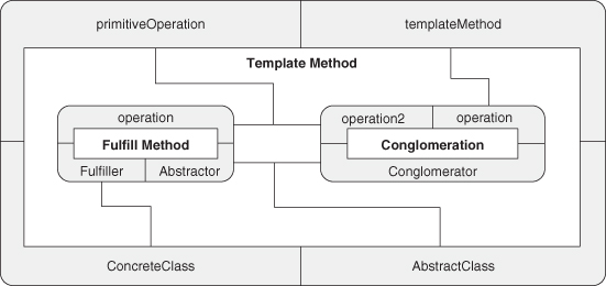
ς-calculus also swept aside everything but the four required and necessary entities—objects, method, fields, and types—opening the way for simple analyses that are truly comprehensive. For example, given only four items to work with, there are only sixteen ways they can be combined. This point was illustrated in Table 2.2, which is reproduced here in Table A.1.
Table A.1. All interactions between entities of object-oriented programming
This table is small enough that we can pick it apart piece by piece. We can address most of this table at one shot by investigating Defines. An object defines a method inside of it, or a field, or perhaps a type. Objects such as namespaces or package objects can also define other objects within them. Methods can, in some languages, define inner methods and types within them but can almost always define objects and fields. Fields, by their nature, do not readily wrap or define other elements, but the type of the field, such as a class, can define any of the four elements.
This defining of inner entities is also known as scoping. A class that defines a method is scoping that method inside itself. You must go through the class to get to the method, either directly or through an object or field instantiated from that class. Objects scope their children, as do methods. Examples of these in C++ include scoping a static method in a class or a field in a namespace: Some-Class::aMethod() and ANamespace::aField respectively. Java eschews the double colon scoping operator and unifies the scoping notation across the board to use a simple dot, as in SomeClass.aMethod() or APackage.aField. This is the same notation that ς-calculus uses. In all cases, scoping is indicated by the dot operator. It should look very familiar to most programmers because it is used both to scope through bound instances and select entities out of a definition. There’s really no difference in practice. In fact, defines is just a synonym for scopes.
So why didn’t I just use Scopes instead? The critical difference between the traditional denotational calculus of procedural programming, λ-calculus, and ς-calculus is that selecting an element from a field brings into play the σ operator. This is what binds an instance to a type, allowing for proper lookup of the selected item out of the scoping provided by the field, even when polymorphism is present. This binding is unique to ς-calculus and, combined with the treatment of objects as first-class entities, is what makes it extremely effective and elegant. We can, however, ignore this binding for the purposes of this text.
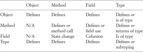
Eliminating defines as a known concept leaves us with Table 2.3, again reproduced here, as Table A.2.
Table A.2. Nonscoping interactions between entities of object-oriented programming
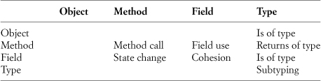
Objects and fields are declared to be “of a type.” ς-calculus displays this as anObject: itsType. This notation is also used to indicate the return type of a method. Types subtype or inherit from one another. This is shown in ς-calculus as Subtype <: Supertype.3 That eliminates the entirety of Table A.2 except for the four reliance operators: method call, field use, state change, and cohesion.
3. Subtyping, subclassing, and inheritance are not all the same from a formal point of view, but for the purposes of this book, we can use the terms interchangeably. See [1] for details.
There are four reliance operators—relops for short—in ρ-calculus, based on the four relationships described above. The method-method relop (that is, a method call) is the mu-form. This is the single reliance operator discussed in this book. The method-field—a field use—is the phi-form. The field-method is a state change—in other words, the state of the field depends on a method call in some manner—known as the sigma-form. Finally, a field-field reliance is the traditional cohesion, or kappa-form. These are denoted in the mathematics of ρ-calculus as <μ, <φ, <σ, and <κ, respectively. The notation comes from the subtyping operator <:, which you can think of as stating, “The subtype relies on the supertype for its existence and intent.” Because : is a typing operator, we can reinterpret < as “relies on.” This basic notation is then subscripted with the appropriate indicator to form the four reliance operators. They are binary operators that form a reliance from the left-hand side of their use on their right-hand side. In other words, someMethod <μ anotherMethod should be read as someMethod relies on anotherMethod.
A.2. Transitivity and Isotopes
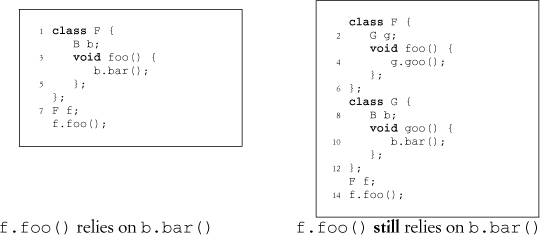
In Section 4.1.1, you learned about isotopes and how they are formed from indirect reliances. We can use ρ-calculus to give this process a formal basis through transitivity. The following source example reproduces our code example from Section 4.1.1. We can state, as before, that f.foo relies on b.bar, but now we can write this as f .foo <μ b.bar. So far, so good. In our example on the right side, we can say that f .foo <μ g.goo and that g.goo <μ b.bar.
We can use these two bits of information in a reduction rule. This is the primary form of inference in ς-calculus and ρ-calculus. Given a set of clauses that we know to be true, we can infer a new property. We say that we are reducing the clauses to the result. For instance, in this case, there is a reduction rule for <μ transitivity, as in Equation A.1.
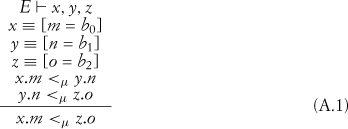
This reduction rule begins by stating that we have an environment E such that we have defined in this environment x, y, and z. The next three clauses state that these elements are defined as having subelements m, n, and o, respectively, which are indicated to be methods. The next two clauses specify relops such that x.m relies on y.n, and y.n relies on z.o. Given this set of clauses, the inferred result is that x.m relies on z.o. This is just one of the many transitivities in ρ-calculus, and they are what give ρ-calculus much of its analytic strength. Extremely large systems can be reduced to simple sets of relops, and the existence of high-level abstractions such as design patterns can be searched for by looking in the simplified views of the results. Without this technique, we would have to continually work with or examine all of the intervening pieces. If, for example, we were looking for proof that x.m called z.o, a simple examination of this system would fail to find it. By using the transitivities of ρ-calculus and stating that we are looking for a situation where x.m relies on z.o instead, we can prove the existence of the relationship quickly and cleanly.
More precisely, this transitivity allows us to create specific reliance-based definitions for design patterns that can match a tremendous number of structural implementations. These are the isotopes of the canonical, most basic and direct implementation. This is what makes this approach so powerful and flexible.
A.3. Similarity
Our three axes of similarity from Section 2.2.2 can likewise be given a formal basis in ρ-calculus. As a quick reminder, there are three possible ways in which a single relop can have similarities between its two sides. For instance, given the reliance f.foo <μ b.bar, we can talk about the object similarity between f and b, the similarity between the types of f and b, and the similarity between the methods foo and bar. We use ~ to indicate similarity in ρ-calculus and ≁ for dissimilarity. For instance, A ~ B for “A is similar to B” or B ≁ C for “B is dissimilar to C.”
The similarity between the types is found in the ρ-calculus definition of f and b. For us to use f and b in a ρ-calculus definition, they must be defined, and they must be given types. Therefore, the typing information of f and b must already be defined. We can talk about this typing relationship, however, as one of the following: unrelated, which we will just call dissimilar, and denote by ≁; the same exact type, which we call similar and mark as ~; subtyping, denoted by the previously seen <:; and sibling typing, in which two types share a common supertype, indicated by <:>. All of this information is already present in ρ-calculus.
We can talk about the similarity between objects and methods as either similar or dissimilar as well, using the same ~/≁ notation. For brevity, however, and because this information is unique to specific reliance operator instances, we can add this information to the reliance operator notation directly as a superscript, albeit in a slightly modified form.
Although the ~/≁ notation is easily distinguishable at normal text sizes, at small font sizes it presents readability problems, so +/– is used instead for clarity.4 The selection notation of the dot operator is mimicked in the similarity notation: the object similarity is placed on the left of a dot and the method similarity is placed on the right. For instance, a method call relop with object dissimilarity and method similarity would be noted as ![]() . A relop with object similarity and method dissimilarity would be shown as
. A relop with object similarity and method dissimilarity would be shown as ![]() , and so on. This lets us collapse a tremendous amount of information into a concise form. Combined with the transitivities, it lets us describe relationships between any two entities in a system quickly, precisely, and cleanly.
, and so on. This lets us collapse a tremendous amount of information into a concise form. Combined with the transitivities, it lets us describe relationships between any two entities in a system quickly, precisely, and cleanly.
4. The ~ and ≁ notations were, pardon the pun, too similar at the small font sizes found in subscripts to be useful in this manner. User feedback led to the adoption of the +/– as a more visible version.
It might occur to you that we may not always know the similarity or dissimilarity between two elements of a system. You are correct. In such cases, a circle, ο, is used to convey a truly unknown relationship.
A.4. EDP Formalisms
We now have the basis for formally defining and working with ρ-calculus to create the foundation for the EDPs. We can revisit the EDP design space diagrams from Section 4.4 and reannotate them with our new notation, as in Figures A.1 and A.2.
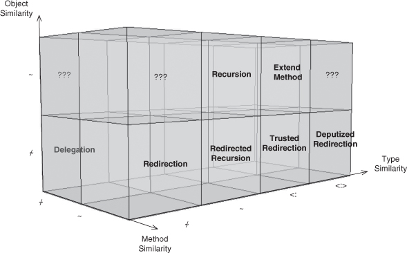
Figure A.1. The full method call EDP design space: similar method.
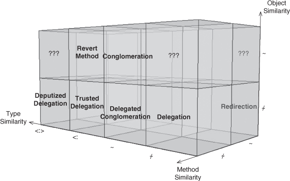
Figure A.2. The full method call EDP design space: dissimilar method.
Let’s establish a simple setup for this discussion. Assume we have an object o of type A and an object p of type B. We can write these as o : A and p : B, respectively. Type A defines a method f and type B defines a method g. This setup could be shown in code something like in Listing A.1.
We can now define the EDPs on the basis of their placement within the design space, using our similarity notation and reliance operators.
Looking at Figure A.1, we can see that Recursion is at the intersection of the axes of object, type, and method similarity. This means that Recursion can be expressed formally as o.f ![]() p.g, A ~ B. Recall that the superscript indicates what the relationship is between the two elements on either side of the matching scoping dot operator. In this case, that o is similar to p and f is similar to g.
p.g, A ~ B. Recall that the superscript indicates what the relationship is between the two elements on either side of the matching scoping dot operator. In this case, that o is similar to p and f is similar to g.
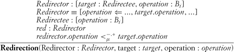
You can see that Delegation can be written as o.f ![]() p.g, A ≁ B, and, as you might expect, Redirection is written o.f
p.g, A ≁ B, and, as you might expect, Redirection is written o.f ![]() p.g. The claim from Section 2.2.4 that Redirection and Delegation together form the concept of coupling can be stated, therefore, as o.f
p.g. The claim from Section 2.2.4 that Redirection and Delegation together form the concept of coupling can be stated, therefore, as o.f ![]() p.g. Our “unknown” notation finally comes into play, albeit in a minor way.
p.g. Our “unknown” notation finally comes into play, albeit in a minor way.
Listing A.1. Simple code example
class A {
2 void f();
};
4
class B {
6 void g();
};
8
A o;
10 B p;
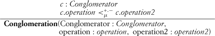
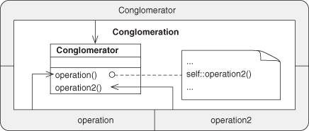
I’m pretty sure you can guess what Conglomeration looks like at this point: o.f ![]() p.g, and now the cohesion discussed in Section 2.2.4 reduces to o.f
p.g, and now the cohesion discussed in Section 2.2.4 reduces to o.f ![]() p.g, as the similarity from Recursion and the dissimilarity from Conglomeration cancel each other out.
p.g, as the similarity from Recursion and the dissimilarity from Conglomeration cancel each other out.
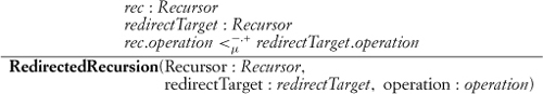
For Redirected Recursion, the method reliance is what you’d expect for a Redirection: o.f ![]() p.g. By the way, this is our formal reasoning for going with Redirected Recursion as a name—this is a refinement of Redirection, not Recursion. As a result, only the type relationship needs to be changed, to A = B.
p.g. By the way, this is our formal reasoning for going with Redirected Recursion as a name—this is a refinement of Redirection, not Recursion. As a result, only the type relationship needs to be changed, to A = B.
For the final two EDPs along the bottom row of Figure A.1, we add our subtyping and sibling relationships. Again, the method reliance is what you’d expect for a Redirection, o.f ![]() p.g, and once more we only change the type relation. This time it is set to A <: B, which indicates that A is a subtype of B, giving rise to the Trusted Redirection EDP.
p.g, and once more we only change the type relation. This time it is set to A <: B, which indicates that A is a subtype of B, giving rise to the Trusted Redirection EDP.
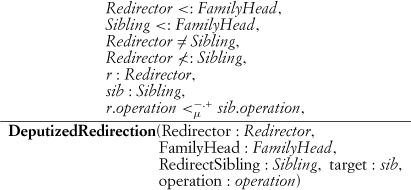
We can arrive at Deputized Redirection by again starting with Redirection, this time making a simple change to the type reliance relationship, such that A <:> B.
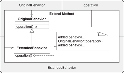
Finally, let’s revisit Recursion. Start with its call reliance operator and type statements: o.f ![]() p.g, o : A, p : B. Change the type relationship to A <: B. That’s all there is to modifying Recursion to evolve it into Extend Method.
p.g, o : A, p : B. Change the type relationship to A <: B. That’s all there is to modifying Recursion to evolve it into Extend Method.
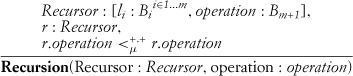
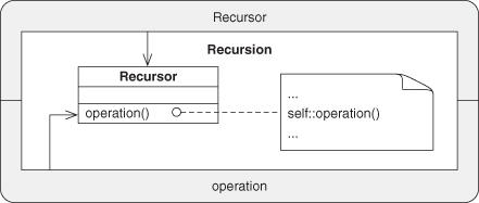
We can use this approach to define any of the EDPs within this design space, elegantly and concisely expressing their core relationships using the ρ-calculus. Section A.7 provides full definitions for each EDP using our reduction rule notation from Section A.2. Given the proper set of clauses, we can infer that the fact at the bottom of a reduction rule is evident and in turn use it as a new clause in other reduction rule inferences. For instance, take the definition for Recursion:
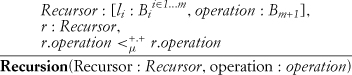
The clauses above the line are analogous to what we saw when we defined Recursion. The first clause states that Recursor is a type and that it has at least one method, which is named operation, with other optional methods and/or fields. The second clause establishes that the object r is of type Recursor. The third clause states that r.operation has a method call reliance on itself, with both object and method similarity. The final line states that the elements in the prior clauses form an instance of Recursion. We use the names in the formal definition as the names of the roles for the pattern. These are used both when discussing the pattern and for defining the structure of its equivalent PIN representation, as you’ll see in Section A.6. The slots that are bound to these roles are variables in the mathematical sense. Once an entity is bound to a role, that role is said to be fulfilled by that entity. In the preceding case, any class that satisfies the needs of Recursion as stated in the definition is said to be bound to the Recursor role of Recursion.
A.5. Composition and Reduction Rules
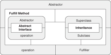
Starting with these definitions, we can compose them into more complex patterns, just like we did in the earlier chapters. Let’s reexamine the building of Decorator that we undertook in Section 4.2. To recap, we introduced Fulfill Method as a combination of Inheritance and Abstract Method, and then used Fulfill Method to define Objectifier. We combined Objectifier and Trusted Redirection to define Object Recursion, which was then brought together with Extend Method to create Decorator.
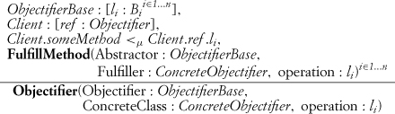
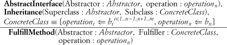
Let’s start by defining Fulfill Method as:

The first clause declares an instance of Abstract Interface, which takes two arguments, the first a type entity, and the second a method entity. It establishes the relationship between them as defined in the Abstract Interface pattern but allows us to replace the full formal definition with this shorter version. The second clause establishes that ConcreteClass is a subclass of Abstractor through an instance of the Inheritance EDP. The third line is the new piece of the puzzle. It states that the method stated in Abstract Interface is defined by ConcreteClass, fulfilling the promise made by Abstract Interface. Note that this piece is crucial, as there is no need for a subclass to actually define the abstract method—it may just be another abstract class in the class hierarchy. The names provided in the clauses are not accidental. If a name appears in more than one position in a reduction rule, then the same entity in the system is being used in each role. This is what ties together the smaller patterns into a larger composition.
We can continue the reduction rules process and define Objectifier by adding a Client class to a plurality of operations to abstract:
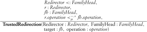
Trusted Redirection looks rather like our earlier definition for Recursion:
The formal definition of Object Recursion is then:
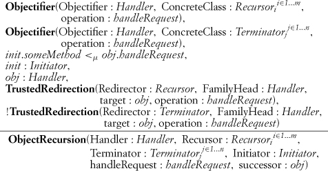
We’re establishing that some Objectifier ConcreteClasses are involved in Trusted Redirection and some are not. If all such classes were involved in redirection, a call into this architecture would never terminate.
Next, we can use a shorthand notation for establishing that an element is a method of a class as in aMethod ∊ meth(aClass) and define Extend Method as:

Finally, we can define Decorator as:

Note that these equations can be correlated closely with the PIN diagrams used in Section 4.2 to illustrate the compositions. In fact, as we’ll see next, PIN and the uses of pattern instances in reduction rules go hand in hand.
A.6. Pattern Instance Notation and Roles
One design goal of PIN is to allow the simple display of composed patterns through expanded PINboxes. The rules for PIN closely mirror those for the reduction rule compositions in this appendix. For instance, Figure A.3 is a repeat of Figure 3.9, and instances of those patterns in the formalism of ρ-calculus would appear as PatternA(Role1 : a, Role2 : b) and PatternB(Role1 : a, Role2 : b, Role3 : c, Role4 : d, Role5 : e, Role6 : f), where a through f represent unbound roles.
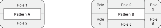
Figure A.3. Standard PINbox.
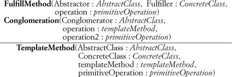
Likewise, Figure A.4 shows our expanded PINbox example from Figure 3.14, which we can now define formally as:
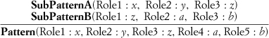
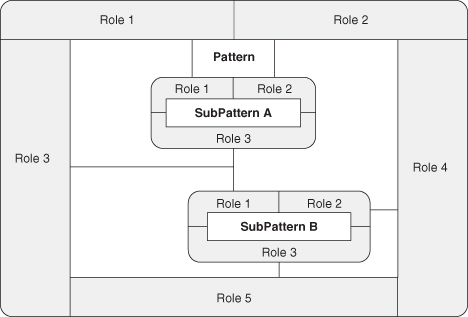
Figure A.4. Expanded PIN instance.
There is a one-to-one correlation between the roles ringing a PINbox and the roles in the formal definition. Also, each connection in the PINbox diagram illustrates a point at which the same bound variable is used in multiple role fulfillments within the definition.
A.7. EDP Definitions
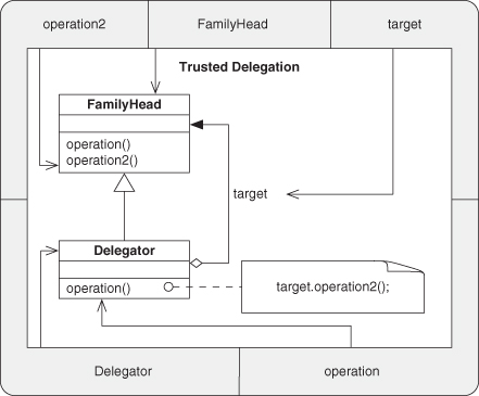
This section provides fully formal definitions of each of the EDPs in this text, using ρ-calculus. Not every aspect of these definitions is explained in full, although you have seen most of the notation used. If you would like a deeper treatment, refer to the base publications for the complete reference, in particular A Theory of Objects [1], which provides the comprehensive foundation you need, as well as SPQR: Formal Foundations and Practical Support for the Automated Detection of Design Patterns from Source Code [35], which provides the original definitions and a much deeper discussion of each. Some minor details have changed since original publication, such as the addition of the explicit naming of the roles in pattern instances. This was found to be of great utility after the original references were published. Each of the following definitions is accompanied by its equivalent PIN diagram so you can immediately see the correlation with the formalism.
A.7.1. Create Object
This definition is the closest to its foundations in ς-calculus, and studying that foundation is recommended if you wish to truly understand this definition in detail. Or, you can accept that this is a very specific definition for a very simple concept.
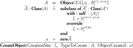
where ![]() (and may be Root), ⌊A⌋ = A for O-1, X <: A for O-2, and X < #A for O-3-compliant languages, respectively, according to the classifications established in [1].
(and may be Root), ⌊A⌋ = A for O-1, X <: A for O-2, and X < #A for O-3-compliant languages, respectively, according to the classifications established in [1].
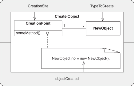
Note that it may very well be easier to consider this as an axiomatic output directly from a language model than to try to derive it from ς-calculus constructs. In particular, if attempting to perform analysis of source code, use the language semantics instead of trying to derive this from ς-calculus primitives.
A.7.2. Retrieve
Most object-oriented languages do not allow the updating of methods with new values (method bodies). Instead, only data fields can be updated in this manner. From a theoretical point of view, there is no appreciable difference between these two scenarios. We allow for both, relying on language semantics to govern which cases are valid and which are not. By deferring our definition until we have a set of well-formed ρ-calculus facts, we avoid much of the complexity of handling the myriad of language quirks. There are two basic forms for the Retrieve pattern:
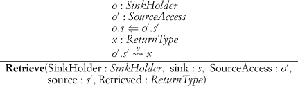

Both forms are composed of an update in the first clause and a return of a value in the second clause, either by name, indicating a shared reference, or by value, indicating a fresh copy.
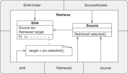
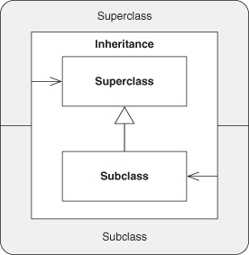
A.7.3. Inheritance
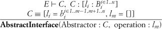
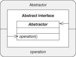
A.7.4. Abstract Interface
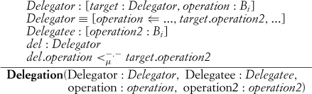
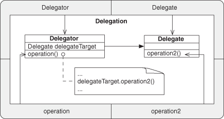
A.7.5. Delegation
A.7.6. Redirection

A.7.7. Conglomeration
A.7.8. Recursion
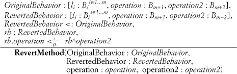
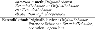
A.7.9. Revert Method
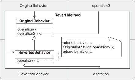
A.7.10. Extend Method
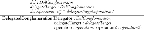
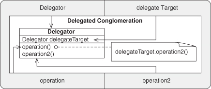
A.7.11. Delegated Conglomeration
A.7.12. Redirected Recursion

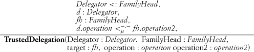
A.7.13. Trusted Delegation
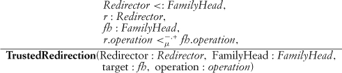
A.7.14. Trusted Redirection

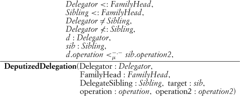
A.7.15. Deputized Delegation
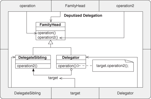
A.7.16. Deputized Redirection

A.8. Intermediate Pattern Definitions
Here you will find the definitions for the patterns presented in Chapter 6. These are the initial patterns demonstrating composition reduction rules from prior pattern instances. Again, each definition is presented along side its equivalent PIN diagram.
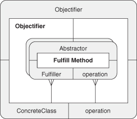
A.8.1. Fulfill Method
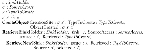
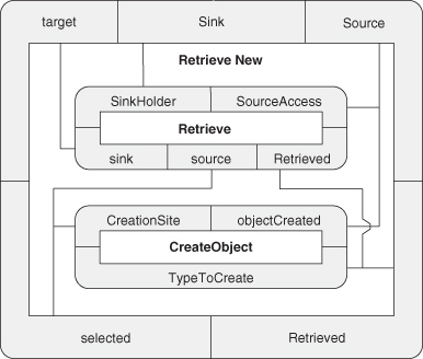
A.8.2. Retrieve New
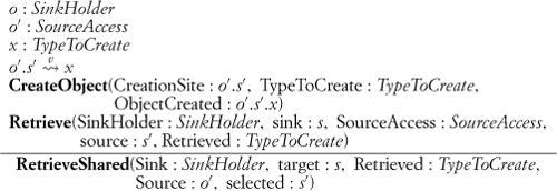
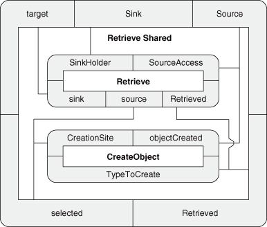
A.8.3. Retrieve Shared
A.8.4. Objectifier

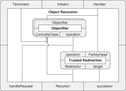
A.8.5. Object Recursion

A.9. Gang of Four Pattern Definitions
Finally, this section presents definitions and PIN diagrams for each of the Gang of Four patterns discussed in Chapter 7.
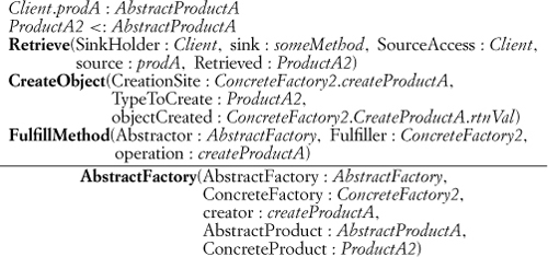
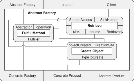
A.9.1. Abstract Factory
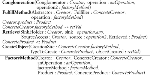
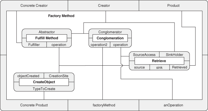
A.9.2. Factory Method
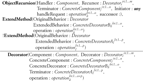
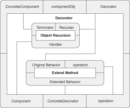
A.9.3. Decorator
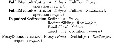
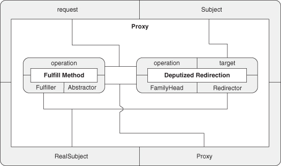
A.9.4. Proxy
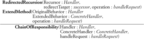
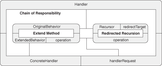
A.9.5. Chain of Responsibility
A.9.6. Template Method