
Structural Equation Modeling of Repeated Measures Data: Latent Curve Analysis
University of North Carolina
The statistical analysis of repeated measures data over time can be a remarkably challenging task that, if successful, has the potential for allowing significant insight into many important theoretical questions of interest. Over the years, a wide variety of longitudinal statistical models have been proposed to address this challenge, including repeated measures t-tests, analysis of variance (ANOVA), analysis of covariance (ANCOVA), multivariate analysis of variance (MANOVA), multiple regression, and path analysis. Advances in structural equation modeling (SEM) over the past 25 years have provided many additional statistical methods for analyzing longitudinal data. One SEM method that has had a long and important history within a wide variety of social science research settings is the autoregressive crosslagged (ARCL) panel model. However, because of several limitations associated with this modeling approach when applied under certain conditions (e.g., Rogosa, 1995), the past decade has witnessed the rise of an alternative SEM-based analytic approach to modeling longitudinal data, the latent curve model. Although latent curve analysis overcomes a number of limitations associated with the ARCL model, it is not without its own limitations. Applied researchers must be able to weigh the advantages and disadvantages of each of these analytic approaches so that an informed decision can be made about the optimal analytic strategy for evaluating the particular research question at hand (Curran & Bollen, in press).
The goal of this chapter is to explicate the advantages and disadvantages of using the SEM-based latent curve model in applied longitudinal research. This will be accomplished both through a discussion of the basic concepts and equations underlying latent curve analysis and through an applied example concerning the development of antisocial behavior in children. We begin the chapter with a description of the theoretical framework, specific hypotheses, empirical sample, and measures that will be used in the applied example. We then briefly review the ARCL model and discuss the potential advantages and disadvantages of this analytic strategy for evaluating longitudinal research hypotheses. We follow this with an introduction to latent curve analysis and a detailed application of these models to a set of theoretically derived research questions. Our primary intent is for this chapter to address the needs of applied researchers by providing a detailed pedagogical introduction to the latent curve model that describes the analytic technique and highlights its advantages, limitations, and potential future directions.
THE DEVELOPMENT OF ANTISOCIAL BEHAVIOR IN CHILDREN
The onset and escalation of antisocial behavior during early childhood can place a child at increased risk for a variety of negative developmental outcomes in adolescence and adulthood, affecting academic attainment, mental health, substance abuse, social adjustment, criminality, and employment success (Caspi, Bem, & Elder, 1989; Loeber & Dishion, 1983; Reid, 1993). Relations between early childhood behavioral problems and later adjustment difficulties unfold in a developmental process (Patterson, Reid, & Dishion, 1992) such that more severe forms of adolescent and young adult conduct problems are likely to be initiated early in childhood and, without intervention, become increasingly difficult to modify over time (Coie & Jacobs, 1993).
The seemingly intractable nature of antisocial behavior indicates that early prevention efforts targeting high-risk children within this developmental process are likely to be our most successful mode of intervention [Conduct Problems Prevention Research Group (CPPRG), 1992; Kazdin, 1993; Reid, 1993]. However, many previous attempts to prevent and treat childhood antisocial behaviors have been ineffective (CPPRG, 1992; Kazdin, 1985, 1987, 1993), and the lack of developmental theory in conceptualizing these interventions has been at least partially implicated as underlying such intervention failures (Cicchetti, 1984; CPPRG, 1992; Dodge, 1986, 1993). The development of antisocial behavior in children is embedded within a series of complex reciprocal relationships among parents, children, and teachers set across the contexts of the home, school, and peer group (see, e.g., CPPRG, 1992; Patterson et al., 1992). For example, previous research has shown that parents may contribute to their children’s academic readiness for school entry by providing both emotional support and a cognitively stimulating home environment for their children (CPPRG, 1992). Children who show lack of academic readiness at school entry often experience greater impediments to learning at school, especially if combined with pre-existing inattentiveness, antisociality, and hyperactivity (Moffitt, 1990).
As the child progresses through school, continued aggressive and antisocial behavior decreases the time children spend on school-related tasks, further delaying the development of academic skills (Patterson, 1982; Patterson et al., 1992; Wilson & Herrnstein, 1985). As a result, conduct-disordered children are more likely to display a number of academic deficiencies, particularly in the development of age-appropriate reading skills (Kazdin, 1993). Although both theory and empirical evidence suggest that, once started, earlier antisocial behavior is associated with later disruptions in academic achievement, it is not known whether there is a reciprocal relation such that earlier academic failure promotes further antisocial behavior (Patterson et al., 1992). Regardless, such skill deficits and ongoing academic failure are likely to result in greater rejection of the antisocial child by peers, teachers, and even parents (Patterson et al., 1992). In turn, social rejection alienates children from positive socializing agents and hinders the development of healthy bonds between a child and his family and school, thereby placing the child at risk for affiliating with deviant peers (Patterson, 1986). These deviant peer affiliations are a key launching pad into further behavioral problems when entering early adolescence (Elliott, Huizinga, & Ageton, 1985).
This developmental model of antisocial behavior is concerned with the early onset and process of change within each individual child’s developmental trajectory over time, emphasizing individual differences in the intraindividual development of antisocial behavior over time. Moreover, these individual trajectories are embedded within the larger developmental context of the child, such that the point of school entry appears to be a critical time to examine change in child antisocial behavior that may be subject to later intervention (Reid, 1993). Several factors, both within the home and school, may alter the course of these trajectories. Finally, academic skills, especially reading, are thought to be involved in the development and maintenance of antisocial behavior in children over time (Kazdin, 1993).
Such questions concerning individual differences in systematic change over time (or individual developmental trajectories) are well suited for evaluation using latent curve analysis. To demonstrate this analytic technique, we examine four theoretical questions based on this developmental model of antisocial behavior. First, is there evidence for systematic change and individual variability in change in antisocial behavior from childhood to adolescence? Second, is the child’s gender or the child’s age related to the initial levels or rates of change in antisocial behavior? Third, is the emotional support and/or cognitive stimulation provided to the child related to the initial levels or rates of change in antisocial behavior? Finally, are earlier levels of antisocial behavior related to later development in reading recognition, and are earlier levels of reading recognition related to later development in antisocial behavior? A series of latent curve models are applied to the empirical data both to better understand these research questions and to provide a detailed example of this analytic strategy.
SAMPLE AND MEASURES
Subjects for the present study were drawn from the National Longitudinal Survey of Youth (NLSY) of Labor Market Experience in Youth, a study that was initiated in 1979 by the U.S. Department of Labor to examine the transition of young people into the labor force. The original 1979 panel included a total of 12,686 respondents, 6,283 of whom were women. Beginning in 1986, an extensive set of assessment instruments was administered to the children of the 6,283 female respondents of the original NLS Youth sample. A total of 4,971 children was assessed in 1986, which represented approximately 95% of those children eligible for interview. These child assessments were again administered every other year following the 1986 interview: 6,266 children were interviewed in 1988, 5,803 in 1990, and 6,509 in 1992. The mothers of the children continued to participate in the NLS Youth annual interviews during this time. As of 1992, at least 1 interview was obtained on 9,360 biological children of the original 6,283 women first interviewed for the NLSY in 1979.
Although a very large number of children of the original NLS Youth mothers was interviewed at least one time to date (N = 9360 by 1992), a much smaller number of mother–child pairs was considered for the present study. Three key criteria were required for inclusion in the sample. First, children must have been between the ages of 6 and 8 years at the first wave of measurement. This choice of age range insured that all children were eligible to be assessed on the measures of interest to the present study. Second, children must have reported complete data on all measures of interest to the present study at the first wave of measurement. Subjects were included in the present sample if they were missing data on some or all measures after the first wave of measurement. Finally, only one biological child was considered from each mother. Based upon these three criteria, a total sample of N = 405 children was considered for the present analyses. All N = 405 children and mothers were interviewed at Time 1, N = 374 were interviewed at Time 2, N = 297 were interviewed at Time 3, N = 294 were interviewed at Time 4, and N = 221 were interviewed at all four assessments. Of the total sample of N = 405, 49.9% were female and the average child age at Time 1 was 6.9 years (sd = .64).
Data for the NLSY Child survey were primarily collected using personal home interviews administered by trained interviewers. Measures used in the present study were a subset drawn from the much larger complete battery of assessments administered to the NLSY mothers and children. Antisocial behaviorAntisocial behavior was measured using the Behavior Problems Index (BPI) antisocial behavior subtest, one of six subtests of the BPI developed by Zill and Peterson (Baker, Keck, Mott, & Quinlan, 1993). The antisocial behavior subscale consisted of the mother’s report on six items that assessed the child’s antisocial behavior having occurred over the previous 3 months. The three possible response options were not true (scored = 0), sometimes true (scored = 1) or often true (scored = 2). These six items were summed to compute an overall measure of antisocial behavior, and scores could range in value from 0 to 12. The child’s reading recognition skill was measured using the 84-item Peabody Individual Achievement Test (PIAT) Reading Recognition subtest, one of five subtests of the PIAT. The reading recognition subtest measures word recognition and pronunciation ability, components considered essential to reading achievement. The reading recognition measure was computed by summing the total number of correct items for the 84-item subtest, and scores could range in value from 0 to 84. The final reading recognition scores were divided by 10 to better equate these variances with the other variables under consideration for later analyses. Antisocial behavior and reading recognition were assessed every other year for four assessments.
Four explanatory variables were of interest to the current paper. Emotional support and cognitive stimulation provided to the child were assessed using the Home Observation for Measurement of the Environment-Short Form (HOME-SF; based on Baker et al., 1993). Emotional support was computed as a summation of 13 dichotomously scored items as reported by the mother and as observed by the interviewer, and scores could range in value from 0 to 13. Cognitive stimulation was computed as a summation of 14 dichotomously scored items as reported by the mother, and scores could range from 0 to 14. Only Time 1 measures of emotional support and cognitive stimulation were considered. Finally, child age was measured in years at Time 1, and child gender was dichotomously scored such that female was coded as zero and male was coded as one.
The means, standard deviations, and correlations for all measured variables are presented in Table 3.1. Given that there was missing data evident at Times 2, 3, & 4, these descriptive statistics are based upon all available cases at that particular time point. A standard statistical analysis of this data would use a listwise deletion procedure in which only cases that had measures on all time points would be included. If this approach were applied here, 45% of the cases (184 of 405) would be deleted. However, recent developments in both statistical theory and available software have provided extremely important options to avoid this significant loss of data. For all models presented here, the newly developed program Mplus (Muthén & Muthén, 1998) was used, which allows for the utilization of a missing data estimator. Drawing on statistical theory described by Little and Rubin (1987), maximum likelihood estimation is used incorporating the EM algorithm that provides proper parameter estimates, standard errors, and an omnibus likelihood ratio (or χ2) test statistic. A full discussion of this method of estimation is beyond the scope of this chapter, but the end result of this approach is the utilization of all available cases at each time point. See Little and Rubin (1987) and Muthén and Muthén (1998) for further details. Prior to applying the latent curve models to the empirical data, we will first present a brief review of the structural equation model followed by an introduction to the ARCL modeling approach.
Table 3.1: Means Standard Deviations, and Correlations for all Measured Variables
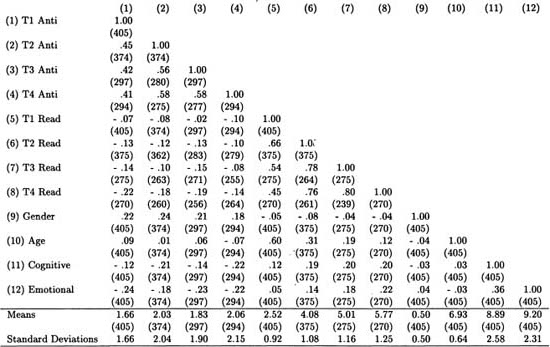
Note: Italicized numbers in parenthesis indicate the available sample size for each pair-wise correlation. Numbers on the horizontal axis of the table refer to variables numbered on the vertical axis of the table. The mean and standard deviation for each variable are reported in the last two lines of the table.
THE STRUCTURAL EQUATION MODELING FRAMEWORK
Structural equation modeling, or SEM, is a term used to define a broad class of multivariate statistical models that are widely used in the social sciences. The SEM approach simultaneously estimates relations between observed variables and the corresponding underlying latent constructs and between the latent constructs themselves (Bentler, 1980, 1983; Jöreskog, 1971a, 1971b; Jöreskog & Sörbom, 1978). From this perspective, the factor analytic model relates the observed variables y to the underlying latent construct η such that
where υ is a vector of measurement intercepts, Λ is a matrix of factor loadings (or measurement slopes), and ε is a vector of measurement residuals. Conceptually, this reflects that the observed measures on y are used to define the unobserved latent construct, or factor, believed to have given rise to the measures. Further, the observed variance in y is partitioned into two parts: (a) that which is explained by the underlying factors and (b) the remainder, which is considered error. Thus, the variance of the underlying factors are theoretically “error free.” Once these factors are estimated, then relations among the factors can be examined such that
where α is a vector of structural intercepts, B is a matrix of structural slopes, and ζ is a vector of structural residuals and V(ζ) = Ψ represents the covariance structure among the latent factors. Thus, Equation 3.1 relates the observed measures to the underlying latent factors, and Equation 3.2 relates the latent factors to one another.
The SEM framework allows for the estimation of a wide array of powerful and flexible statistical models that can be applied to test research hypotheses in many areas of social science research. Although a comprehensive review of all such techniques is beyond the scope of this chapter, more detailed discussions of these models can be found in Dwyer (1983) and Windle (1997). However, two longitudinal SEMs that have received significant recent attention are the autoregressive crosslagged (ARCL) model and the latent curve model. We next provide a brief review of the ARCL model followed by a more detailed discussion of the latent curve model.
THE AUTOREGRESSIVE CROSSLAGGED MODEL
Our analytic goal is to empirically evaluate the four research questions described earlier. One technique available to accomplish this is the ARCL modeling strategy. The ARCL approach is based on the classic simplex model developed by Guttman (1954) and extended by Anderson (1960), Humphreys (1960), Heise (1969), and Jöreskog (1979). This modeling strategy incorporates two main components. First, later measures of a construct are predicted by earlier measures of the same construct, thus giving rise to the term “autoregressive.” For example,
indicating that the measure of antisocial behavior for individual i at time point t is an additive combination of a time specific intercept (µt), a weighted contribution of the prior measure of antisocial behavior (ρt), and an individual and time specific random error (εit). Larger positive values of the regression parameter are usually interpreted as indicating greater stability of the construct over time (but see Rogosa, 1995, for concerns about this interpretation), that is, on average, scores above the mean at time t tend also to be above the mean at time t + 1.
Whereas the model described in Equation 3.3 is univariate (given that the repeated measures of only a single construct is considered), this can be extended to a multivariate model in which two or more constructs are examined simultaneously. Here, not only are the later measures of one construct regressed upon earlier measures of the same construct but the later measures of one construct are also regressed on earlier measures of other constructs as well. For example, the measures of reading recognition could be incorporated such that
indicating that later measures of antisocial behavior are a function of an intercept, the weighted contribution of the prior measure of antisocial behavior, the weighted contribution of the prior measure of reading recognition, and a random error term. The model in Equation 3.4 thus has both the autoregressive component as before, but now also has the crosslagged prediction such that earlier measures of reading predict later measures of antisocial behavior. This is sometimes referred to as a residualized change model given that earlier measures of reading recognition predict later measures of antisocial behavior above and beyond the effects of earlier antisocial behavior. This model can be extended to examine bidirectional relations such that earlier measures of antisocial behavior predict later measures of reading recognition as well.
Despite the widespread use of the ARCL modeling approach in many areas of social science research, this analytic technique has been subjected to a great deal of criticism. Critiques address both statistical and theoretical aspects of the model, and many of these are articulated in Rogosa (1995), Rogosa and Willett (1985), and Willett (1988). Briefly, there are three primary concerns within ARCL modeling when addressing hypotheses similar to our four research questions. First, the ARCL is a fixed effects model, meaning that a single value is estimated for the regression parameters (e.g., the ρ’s) that holds for all subjects in the sample. As such, the magnitude of these influences does not vary across individuals, often an unrealistic condition to impose upon the model. Second, the observed mean structure is usually omitted from the ARCL model, thus ignoring potentially important information about mean changes over time. Although means can be introduced into the ARCL model (as was shown in Equations 3.3 and 3.4), it is difficult to explicitly model the structure of the means as a function of time. Finally, changes in the construct between two time points is independent of the influence of both earlier changes and later changes in the same construct. So, change between Times 2 and 3 does not consider change between Times 1 and 2 nor change between Times 3 and 4. This approach thus tends to “chop up” multiple repeated measures into a series of two-time point comparisons, which is often not consistent either with substantive theory nor with the structure of the observed empirical data.
LATENT CURVE ANALYSIS
Given these limitations, there has been a call for the development of alternative statistical models for analyzing repeated measures over time. One particularly promising technique is often referred to as latent curve analysis. Although the historical roots underlying the latent curve model can be traced back to the seminal work of Tucker (1958) and Rao (1958), the SEM-based latent curve model was first proposed by Meredith and Tisak (1984) and formalized by Meredith and Tisak (1990). This was further developed and expanded upon in a variety of important ways by McArdle (1986, 1988, 1989, 1991), McArdle and Epstein (1987), Muthén (1991, 1993, in press), and Muthén and Curran (1997), among many others. Examples of recent substantive applications using latent curve analysis includes Curran and Bollen (in press), Curran and Muthén (1999), Curran, Stice, and Chassin (1997), Duncan, Duncan, and Hops (1996, 1998), and Stoolmiller (1994).
Latent curve analysis draws on the many strengths of the structural modeling framework. One of the basic concepts in structural modeling is that, although we have a set of observed measures of a theoretical construct of interest (e.g., “antisocial behavior”), we are not inherently interested in this set of observed measures. Instead, we are interested in the unobserved latent factor that is thought to have given rise to the set of observed measures. Similarly, within the latent curve framework we are not inherently interested in the observed repeated measures of the construct over time. Instead, we are interested in the unobserved factors that are hypothesized to underlie these repeated measures. However, unlike in the standard SEM factor model where we would like to estimate the latent factor of say “antisocial behavior”, in the latent curve model we would like to estimate latent factors that represent the growth trajectories thought to have given rise to the repeated measures over time. McArdle and Epstein (1987) nicely described these as chronometric factors. So, instead of evaluating the repeated measures from the ARCL framework in which the relations among the observed variables are examined between Time 1 and Time 2, and then between Time 2 and Time 3, and so on, the latent curve model attempts to smooth over the observed measures to estimate the continuous trajectory that gave rise to these time specific observed measures. This conceptualization highlights the elegance of the SEM framework in the estimation of these unobserved growth factors that generated the observed repeated measures. Instead of focusing our explicit interest on the observed repeated measures themselves, we instead use these observed measures to estimate an unobserved latent component thought to underlie our set of measures. Once estimated, the key focus of the analyses is then on these unobserved components of growth.
To better understand the basics of the latent curve model, we now progressively explore the research questions about the relation between antisocial behavior and reading recognition described previously. We first present the equations that describe the various latent curve models and then apply these models to the empirical data and interpret the resulting findings. We start by examining the characteristics of developmental trajectories in antisocial behavior over an 8-year period. We then extend this model to include our four explanatory variables of interest and explore several options available for including the influences of reading recognition. Developmental trajectories in reading will then be examined, and this model will be combined with the antisocial behavior latent curve model to evaluate a comprehensive developmental model of the relations between these two constructs. Finally, we discuss limitations of this modeling approach along with interesting directions for future research.
LATENT CURVE MODELING OF THE PROPOSED RESEARCH QUESTIONS
To summarize thus far, the ARCL model approaches the analysis of the repeated measures data in a series of two-time point comparisons. Regardless of how many assessments are made, the relations among the constructs are examined between time t and time t + 1. The latent curve model approaches the analysis of the repeated measures data in a rather different way. Instead of focusing on specific time adjacent comparisons, the latent curve model uses the SEM analytic framework to estimate the growth factors believed to underlie the observed measures. It is these growth factors that then become of primary interest for later analysis.
To accomplish this, the observed repeated measures of antisocial behavior are expressed as
where λt = 0, 1, 2, 3 for T = 4 assessments. In other words, Equation 3.5 reflects that the observed measure of antisocial behavior for each person i at time point t is expressed as an additive combination of the individual’s own intercept (ηαi), their own slope (ηβi) multiplied by the coefficient of time ((λt), and an individual and time specific random error (εit). Note the subscripting used on these latent factor η’s. First, both the intercept and slope are subscripted with an i indicating that these values are allowed to vary across individuals. This helps overcome one of the limitations of the ARCL model in which one parameter estimate was used to represent the stability of the construct for all individuals. Further, there is not a subscript of t on either the intercept or slope indicating that, although these influences are individually specific, they are independent of time. This means that the observed repeated measures taken at each time point t have been used to estimate the underlying growth trajectories that are independent of t.
What this modeling strategy thus provides is a way of expressing the individual intercept and slope components of growth as a function of group and individual influences. These are expressed as
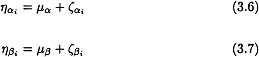
indicating that an individual’s own intercept and slope can be expressed as an additive function of an overall mean intercept (μα) and mean slope (μβ) for the entire sample plus the individual’s own deviation from each of these mean values. The mean values are sometimes referred to as fixed effects and the deviation values as random effects. This formulation accomplishes two important things. First, the observed repeated measures of antisocial behavior have now been smoothed over to provide an estimate of the trajectories thought to underlie the repeated measures. Second, the variance of the deviation terms in Equations 3.6 and 3.7 is a direct estimate of the degree of individual variability in the intercepts and slopes within the sample; the greater the variance, the greater the individual differences in starting point and rates of change over time. This model is often referred to as an unconditional model given that there are no predictor variables on the right hand side of Equations 3.6 and 3.7, that is, variance in the intercept and slope factors are not modeled as a function of other explanatory variables. We will see in a moment that these equations can easily be extended to incorporate predictors of the individual differences in these developmental trajectories.
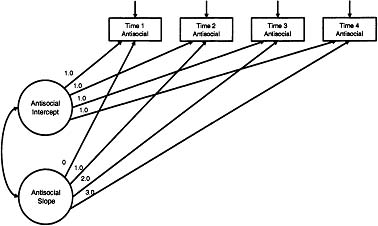
Figure 3.1: Unconditional univariate latent curve model of antisocial behavior.
As a starting point for the analysis, the unconditional univariate latent curve model presented in Equations 3.5, 3.6, and 3.7 was fit to the sample data (see Figure 3.1). This model will provide initial insight into the first research question relating to the characteristics of developmental trajectories in antisocial behavior prior to introducing additional explanatory measures of interest. For this and all subsequent analyses, model fit was evaluated using the following criteria: the relative magnitude of the omnibus χ2 test statistic and the associated p-value where small χ2 values indicate better model fit; the root mean squared error of approximation (RMSEA; Browne & Cudeck, 1993) accompanied with a 90% confidence interval (CI90) where values falling below about .05 to .08 indicate better model fit; examination of modification indices that are 1 df tests of improvement in model fit associated with the freeing of a particular parameter; and examination of covariance and mean structure residuals as indication of potential local misspecification (see Curran, 2000, for further discussion of assessing model fit). Other traditional incremental goodness-of-fit indices are not available due to the use of the missing data estimator.
Using these fit criteria, we concluded that the unconditional latent curve model for antisocial behavior fit the data moderately well [χ2(5) = 14.9, p = .01; RMSEA = .07, CI90 = .03, .11, p(RMSEA < .05) = .18]. There was a significant mean estimate for both the intercept (![]() α = 1.7) and slope (
α = 1.7) and slope (![]() β = .15) factors, indicating that, on average, the group was reporting significant initial antisocial behavior of 1.7 units and significant linear increases of .15 units per time point. Further, there was a significant variance estimate for both the intercept (
β = .15) factors, indicating that, on average, the group was reporting significant initial antisocial behavior of 1.7 units and significant linear increases of .15 units per time point. Further, there was a significant variance estimate for both the intercept (![]() α = 1.29) and slope (
α = 1.29) and slope (![]() β = .133) factors, indicating that there was meaningful individual variability around both of these group level estimates. Thus, some children were reporting high levels of initial antisocial behavior whereas others were reporting lower levels, and some children were reporting steep increases in antisocial behavior over time, whereas others were reporting no increases at all. Finally, there was a marginally significant correlation between the intercept and slope factors (
β = .133) factors, indicating that there was meaningful individual variability around both of these group level estimates. Thus, some children were reporting high levels of initial antisocial behavior whereas others were reporting lower levels, and some children were reporting steep increases in antisocial behavior over time, whereas others were reporting no increases at all. Finally, there was a marginally significant correlation between the intercept and slope factors (![]() αβ = .36) suggesting that children who reported higher initial levels of antisocial behavior also tended to report steeper increases in antisocial behavior over time.
αβ = .36) suggesting that children who reported higher initial levels of antisocial behavior also tended to report steeper increases in antisocial behavior over time.
These modeling results indicate that developmental trajectories thought to underlie the four repeated measures of antisocial behavior are characterized by both significant fixed and random effects. Because we found significant individual variability in the intercept and slope factors, we may now introduce our four explanatory variables to try to predict this observed variability. To accomplish this, Equation 3.5 remains the same, but Equations 3.6 and 3.7 are extended to include the effects of our predictor variables of interest such that:
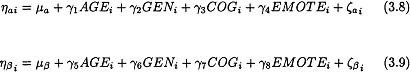
This model is often referred to as a conditional growth model because individual differences observed in the initial starting point and rate of change over time in antisocial behavior are being modeled as a function of the child’s age, gender, and cognitive and emotional support in the home. Note that the explanatory variables are denoted with a subscript i to clarify that these values vary across individuals, but the variables are not denoted with a t to denote time. This is because all of the variables were measured only at the first time point. Variables such as these are often referred to as time-invariant covariates to denote that they do not vary as a function of time (Bryk & Raudenbush, 1992). Note also that the regression parameters linking the explanatory variables to the growth factors (e.g., the eight γ parameters) are not subscripted by i, indicating that these values are estimated pooling over all individuals.
The path diagram corresponding to Equations 3.8 and 3.9 is presented in Figure 3.2. This model was estimated and found to fit the data moderately well [χ2(13) = 25.2, p = .02; RMSEA = .05, CI90 = .02, .08, p(RMSEA < .05) = .50]. Results indicated that gender, age, and emotional support all significantly predicted the intercept factor such that boys, older children, and children with lower emotional support at home reported higher initial levels of antisocial behavior. Further, age and cognitive support significantly predicted the slope factor, indicating that younger children and children with lower cognitive stimulation at home reported steeper increases in antisocial behavior over time. Taken together, the set of four explanatory variables accounted for 27% of the observed variance in the intercept factor and 11% of the observed variance in the slope factor.
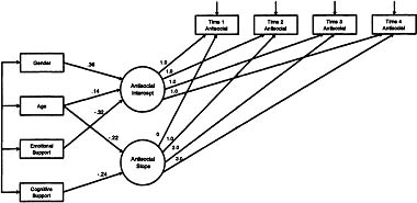
Figure 3.2: Conditional univariate latent curve model of antisocial behavior with four exogenous variables. All paths between exogenous variables and growth factors were estimated, but only significant (p < .05) paths are displayed. Values associated with each path are standardized regression coefficients.
We have found thus far that there are significant initial levels of antisocial behavior, there are significant linear increases in antisocial behavior over time, there is significant individual variability in both starting point and rate of change, and this variability can be modeled as a function of our four explanatory variables. In addition to these important questions, recall that one of our key interests is to better understand the relation between antisocial behavior and reading recognition over time. One option would be to include the Time 1 measure of reading recognition in Equations 3.8 and 3.9 and thus be able to draw the same type of conclusions that were drawn for the other four predictors. However, this is not ideal given that we would be ignoring the latter three measures of reading recognition, thus disposing of a great deal of important information. A better option would be to treat the repeated measures of reading as a time varying covariate. Here, instead of considering the effects of Time 1 reading on the underlying growth trajectories of antisocial behavior (as would be accomplished by including Time 1 reading in Equations 3.8 and 3.9), we instead can introduce the effects of reading on antisocial behavior into Equation 3.5. This is given as
indicating that the observed measure of antisocial behavior for person i at time t is a function of the underlying intercept factor, the underlying slope factor, and the time-specific reading recognition score for person i at time t. The model in Equation 3.10 is nearly equivalent to the time-varying covariate model within the HLM framework (Bryk & Raudenbush, 1992, Equation 6.21). The gamma (γ) parameter estimates in Equation 3.10 would indicate the unique effects of reading directly upon the time-specific measures of antisocial behavior above and beyond the effects of the underlying developmental trajectory of antisociality. Although Equation 3.10 limits a cross-sectional relation between reading and antisocial behavior, Curran, Muthén, and Harford (1998) describe extensions to the latent curve model that allows for the longitudinal prediction from the time varying covariates as well.
The model described in Equation 3.10 (extended to allow for the longitudinal effects of reading on antisocial behavior) is presented in Figure 3.3. This model was estimated and found to fit the data well [χ2 (19) = 29.1, p = .06; RMSEA = .05, CI90 = 0, .06, p(RMSEA < .05) = .80]. Prior to interpretation of the final results, equality constraints were imposed across the regression parameters relating each reading measure to all later antisocial measures (e.g., the regression of all four measures of antisocial behavior on Time 1 reading were set to be equal). These constraints were imposed to evaluate if the regression parameters were of the same magnitude across all time points, and these constraints were not associated with a significant decrement in model fit and were thus retained. The final model fit the data well [χ2 (25) = 36.9, p = .06; RMSEA = .06, CI90 = 0, .06, p(RMSEA < .05) = .87]. All the results relating the growth factors to the four explanatory variables remained nearly identical to those found for the previous model. Interestingly, the Time 1 measure of reading recognition was significantly and negatively associated with all four measures of antisocial behavior, although no significant relations were found for the Time 2, 3, or 4 reading recognition assessments. This indicates that higher levels of Time 1 reading recognition were associated with lower levels of antisocial behavior above and beyond the effects of the developmental trajectory underlying antisocial behavior. However, the results suggest that, once the effects of Time 1 reading recognition are considered, later measures of reading exerted no unique effect on antisocial behavior.
Although this model provides initial evidence that there is indeed some longitudinal relation between reading recognition and antisocial behavior over time, two key limitations remain. First, both developmental theory and previous research would strongly suggest that reading recognition itself is characterized by an underlying developmental process that is clearly not being modeled here. Given that significant intercept and slope factors were found to underlie the four measures of antisocial behavior, it is important that a similar process be examined for reading recognition. Second, although earlier reading recognition was found to predict later antisocial behavior, this model does not evaluate the effects of earlier antisocial behavior on later reading recognition. The model must be further extended to allow for the introduction of both of these important characteristics. Prior to estimating this more complicated latent curve model, we must first take a step back and estimate a univariate model to examine the developmental trajectories in reading recognition. This is because we must first accurately understand the unconditional growth process of reading recognition prior to examining the relation of this process with other influences of interest (see, e.g., MacCallum, Kim, Malarkey, & Kielcolt-Glaser, 1997).
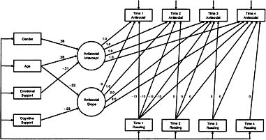
Figure 3.3: Conditional univariate latent curve model of antisocial behavior with effects of reading as a time varying covariate. All paths between exogenous variables and growth factors were estimated, but only significant (p < .05) paths are displayed. All paths between time varying covariates and repeated measures of antisocial behavior were estimated, and non-significant paths are denoted with a value of zero. All other values associated with each path are standardized regression coefficients.
We thus repeat the unconditional latent curve model presented in Equation 3.5 with the simple modification that instead of modeling the four repeated measures of antisocial behavior, we consider the four repeated measures of reading recognition. This is given as
It is extremely important to appreciate the differences between Equations 3.10 and 3.11. Placement of reading recognition on the right side of Equation 3.10 indicates that these measures are treated as independent variables and are used to predict the time specific measures of antisocial behavior. However, reading recognition is placed on the left side of Equation 3.11 indicating that these measures are now dependent variables such that the observed scores depend upon the influences of the underlying growth trajectories.
This model was estimated and was found to fit the observed data extremely poorly [χ2(5) = 175.04, p < .001; RMSEA = .29, CI90 = .25, .33, p(RMSEA < .05) < .001]. Although significant parameter estimates were found for both the fixed and random effects of the intercept and slope factors, these cannot be interpreted given the remarkably poor fit of the overall model. Further information is needed to better understand this lack of fit. First, an examination of the observed means and variances of the four reading recognition scores indicates that, although there appears to be a monotonic increase in these measures as a function of time, the increment of increase is not equal across time. For example, there is a 1.5-unit increase in the means from Times 1 to 2, a 1.0-unit increase from Times 2 to 3, and a .70-unit increase from Times 3 to 4. Thus, it appears that the pattern of mean change over time is curvilinear, whereas the model estimated in Equation 3.11 forces the functional form of the developmental trajectory to be linear (e.g., λt = 0, 1, 2, 3). Large and significant modification indices (1 df tests that evaluate the degree of improvement in model fit if some of the fixed factor loadings were to be freed) provided further support that the source of model misfit stems from imposing a linear growth function on data that demonstrate a strong curvilinear pattern of change.
There are three general options for dealing with this nonlinear form of growth. The first is to simply ignore the issue and move ahead with the analyses. However, we cannot stress strongly enough how ill advised this choice can be. Given that the latent curve model is incorrectly specifying the pattern of growth that is evident in the observed data, no inferences can be made about any aspect of this model given the likely bias that exists throughout many (if not all) of the parameter estimates. Thus, if there is a significant curvilinear trend in the data, it is imperative that this be incorporated in some way into the model.
The second choice is to retain the intercept and linear growth factor, but to add a third factor to account for the nonlinear component in the trajectory (see, e.g., Willett & Sayer, 1994). To accomplish this, Equation 3.11 is extended to add this third factor such that
where λt = 0, 1, 2, 3 as before, and ![]() = 0, 1, 4, 9. Now ηαi represents the intercept, ηLi represents the linear component of the trajectory, and ηQi represents the curvilinear component of the trajectory. Then, just as was done in Equations 3.8 and 3.9, the intercept, linear, and curvilinear components of growth can be regressed upon our four explanatory variables. The model in Equation 3.12 was fit to the observed data and, although the inclusion of the quadratic factor led to a drastic improvement in fit over the linear-only model, the overall model still did not adequately reproduce the observed data [χ2(1) = 10.65, p < .001; RMSEA = .15, CI90 = .08, .24, p(RMSEA < .05) < .01]. Examination of the fixed effects indicated a significant positive intercept, a significant positive linear component, and a significant negative curvilinear component. These parameters are consistent with what we would have expected given the pattern of the observed means. However, although there was a significant random component for the intercept and linear factors, there was a near zero random component for the quadratic factor. This suggests that, although there is a curvilinear component of growth for the overall group, there is not significant individual variability in these curvilinear rates of change. Given the nonsignificant variability in the curvilinear component of growth, we re-estimated this model fixing the variance of the quadratic factor to zero as well as the covariances of the quadratic factor with the other two growth factors (as described by Bryk & Raudenbush, 1992). This resulted in an equally poor fit to the observed data [χ2(4) = 28.0, p < .001; RMSEA = .12, CI90 = .08, .17, p(RMSEA < .05) < .002]. It appears, then, that the quadratic model does not adequately represent the four repeated measures of reading recognition.
= 0, 1, 4, 9. Now ηαi represents the intercept, ηLi represents the linear component of the trajectory, and ηQi represents the curvilinear component of the trajectory. Then, just as was done in Equations 3.8 and 3.9, the intercept, linear, and curvilinear components of growth can be regressed upon our four explanatory variables. The model in Equation 3.12 was fit to the observed data and, although the inclusion of the quadratic factor led to a drastic improvement in fit over the linear-only model, the overall model still did not adequately reproduce the observed data [χ2(1) = 10.65, p < .001; RMSEA = .15, CI90 = .08, .24, p(RMSEA < .05) < .01]. Examination of the fixed effects indicated a significant positive intercept, a significant positive linear component, and a significant negative curvilinear component. These parameters are consistent with what we would have expected given the pattern of the observed means. However, although there was a significant random component for the intercept and linear factors, there was a near zero random component for the quadratic factor. This suggests that, although there is a curvilinear component of growth for the overall group, there is not significant individual variability in these curvilinear rates of change. Given the nonsignificant variability in the curvilinear component of growth, we re-estimated this model fixing the variance of the quadratic factor to zero as well as the covariances of the quadratic factor with the other two growth factors (as described by Bryk & Raudenbush, 1992). This resulted in an equally poor fit to the observed data [χ2(4) = 28.0, p < .001; RMSEA = .12, CI90 = .08, .17, p(RMSEA < .05) < .002]. It appears, then, that the quadratic model does not adequately represent the four repeated measures of reading recognition.
The third option that we consider is to return to the intercept and linear growth factor model presented in Equation 3.11, but instead of fixing the factor loadings to 0, 1, 2, & 3 as we did before, we fix the first two loadings to 0 and 1 (to set the metric of the slope factor), but we will freely estimate the second two loadings from the data. This approach was described by McArdle (1989), who proposed this completely latent curve model to allow for “stretching” and “shrinking” of the time measure to account for nonlinearity in the observed data. We estimated this model and found it to fit the observed data quite well [χ2(3) = 4.4, p = .22; RMSEA = .03, CI90 = 0, .10, p(RMSEA < .05) = .58]. The first two factor loadings were fixed to 0 and 1, and the third and fourth loadings were estimated to be 1.6 and 2.1, respectively. There were significant and positive fixed and random effects for both the intercept and slope factors. The interpretation of the significant fixed effect for the slope factor is that there is a large positive increase in reading recognition over the four time points, but the magnitude of increase diminishes as a function of time. Further, the significant random effects indicate that there is substantial individual variability in both the initial starting point and rate of change over time. We thus conclude that this final model best characterizes the observed mean and covariance structure in the four repeated measures of reading recognition.
Now that we better understand the characteristics of the developmental process underlying reading recognition, we are ready to combine this univariate latent curve model with the latent curve model estimated for antisocial behavior described earlier. Given that we are also interested in the influences of the four explanatory variables, these will be included as well. We thus estimated a single multivariate latent curve model that included the four repeated measures of antisocial behavior and the underlying growth factors, the four repeated measures of reading recognition and the underlying growth factors, and the four explanatory variables. The intercept and slope factors were allowed to covary within construct, the intercept factors were covaried across construct, the slope factors were covaried across construct, each slope factor was regressed upon the intercept factor across construct, and the residual variances of the repeated measures were covaried within each time point. Finally, all four growth factors were regressed upon the four explanatory variables of gender, age, cognitive stimulation and emotional support. We estimated this model and found it to fit the data very well [χ2(35) = 49.8, p = .05; RMSEA = .03, CI90 = 0, .05, p(RMSEA < .05) = .93]. This model is presented in Figure 3.4 in which only significant (p < .05) regression parameters are shown for sake of clarity.
Of initial interest are the relations among the latent growth factors. There was a marginally significant (p < .10) negative correlation between the residual variance of the intercept factor for antisocial behavior and the residual variance of the intercept factor for reading recognition. This suggests that, after estimating the influences of the exogenous variables, children reporting higher levels of initial antisocial behavior also tended to report lower levels of initial reading recognition. Further, the antisocial behavior intercept factor negatively predicted the reading recognition slope factor, indicating that children reporting higher initial levels of antisociality also tended to report less steep increases in reading over time. However, a similar relation was not found between earlier reading recognition predicting later changes in antisocial behavior. This latter finding is quite interesting given the results of the time-varying covariate model (e.g., Equation 3.10) in which Time 1 reading was found to modestly predict later antisociality. This discrepancy in findings highlights the importance of articulating precisely what type of change is of most interest. The time-varying covariate model indicated that Time 1 reading negatively predicted later time-specific levels of antisociality after controlling for the underlying developmental trajectories of antisociality. In contrast, the final latent curve model indicates that earlier reading recognition is not reliably associated with later developmental trajectories of antisociality. So, the former is examining the relation while controlling for antisocial trajectories, and the latter is examining the relation with the antisocial trajectories. These are not necessarily contradictory findings, but instead are different insights into different questions.
Also of interest is the relation between the four explanatory variables and the four growth factors. To summarize, boys were found to report higher initial levels of antisocial behavior, but not differences in any of the other growth factors. Older children were found to report higher initial levels and less steep increases in both antisocial behavior and reading recognition. Higher levels of cognitive stimulation were associated with less steep increases in antisocial behavior and, although higher levels of cognitive stimulation were associated with higher levels of initial reading recognition, cognitive stimulation was not associated with rates of change in reading recognition. Finally, higher levels of emotional support were associated with lower initial levels of antisocial behavior and were thus indirectly associated with later changes in reading recognition as mediated through the antisocial intercept. The results of this final model thus allow for a number of interesting insights into the fourth theoretically derived research question described earlier.
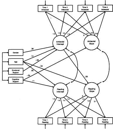
Figure 3.4: Final multivariate conditional trajectory model with exogenous variables. All paths between exogenous variables and growth factors were estimated, but only significant (p < .05) paths are displayed. Values associated with each path are standardized regression coefficients.
CONCLUSIONS
The goal of this chapter was to review the basics of latent curve analysis and to present an extended example demonstrating the analysis of individual differences in rates of change over time. The motivating substantive example for these analyses was an examination of the relation between developmental trajectories of antisocial behavior and reading recognition and the relation between these trajectories and child age, gender, emotional support, and cognitive stimulation. Drawing on theories of developmental psychopathology, four research questions of key interest were identified. These questions related to individual and group characteristics of developmental trajectories in antisocial behavior, in reading recognition, between trajectories of antisocial behavior and reading recognition, and between these developmental trajectories and measures of age, gender, emotional support, and cognitive stimulation. We estimated a series of latent curve models that allowed for inferences to be drawn about all four questions of interest. Specifically, both antisocial behavior and reading recognition were found to be characterized by underlying intercept and slope factors, and there were significant group and individual components of growth. Initial starting points of antisocial behavior and reading recognition were negatively related such that children reporting higher initial levels of antisocial behavior also tended to report lower levels of initial reading recognition. Further, although higher initial levels of antisocial behavior were associated with less steep increases in reading recognition, initial reading recognition was not reliably associated with later increases in antisocial behavior. Finally, interesting relations were found between developmental trajectories of both antisocial behavior and reading recognition and the set of four explanatory variables. Taken together, these results provide important information about the characteristics and predictors of developmental trajectories of antisocial behavior and reading recognition over an 8-year period.
We believe that the latent curve modeling framework provides a number of potential advantages to the empirical study of repeated measures data over time. First, this approach is much more consistent with many types of theoretical questions of development and change compared to the ARCL model. This is because many developmental questions are inherently interested in the continuous underlying trajectories that vary across individual, not necessarily the time-specific levels of a particular measure. However, the ARCL approach can be advantageous in some settings, and recent work has moved toward integrating elements of both the ARCL and latent curve model into a single modeling framework (e.g., Bollen & Curran, 1999; Curran & Bollen, in press). Second, the latent curve model can easily be extended in a variety of interesting ways using the strength of the SEM framework. For example, multiple indicator latent factors could be used to model measurement error within each time point (e.g., Sayer, in press). Additional variables could be examined as potential mediators between the explanatory variables and the growth factors or between the growth factors themselves (e.g., Muthén & Curran, 1997). Multiple group analysis could be used to examine the potential moderating influences of discrete measures such as gender or ethnicity (see, e.g., Curran et al., 1997; McArdle, 1989). Indeed, most any advantage offered by the general structural modeling framework is applicable to the latent curve model.
Having said that, there are, of course, a number of limitations of the latent curve modeling approach as well, and these should be closely considered prior to adopting this technique in practice. First, as with all growth modeling approaches, latent curve analysis requires a minimum of three time points to estimate individual variability in growth trajectories. These models cannot be used for two time point comparisons. Second, although recent advances in software have allowed for the inclusion of partially missing data, the maximum likelihood estimator used here still assumes multivariate normal distributions, both for the repeated measures data as well as the distributions of the latent growth factors. This poses a problem in many areas of research such as child drug use or psychiatric symptomatology where distributions are expected to be significantly skewed. Third, when predicting the growth factors in latent curve analysis, the intercept and slope components are considered separately from one another, thus making interpretation sometimes difficult. For example, the models presented here discussed predictions of the slope factor, but this did not simultaneously consider the corresponding intercept level. Considering both the height and the rate of change of the trajectory simultaneously may be very important information to consider in many research applications. Finally, it remains difficult to evaluate the latent curve models in multilevel settings. For example, in the models presented here we assume that all of the children are independent from one another. However, there are many situations in which children might be nested within a higher level such as classroom or treatment condition, and this can pose a challenge for latent curve analysis (but see Muthén & Muthén, 1998, for new developments in this area).
In conclusion, latent curve analysis is one example of a new generation of statistical models that is well suited for evaluating research questions about repeated measures data over time. The latent curve framework is extremely flexible and can be applied across a variety of applied research settings. Recall that all of the previous equations distinguished both i for individual and t for time. Although “individual” referred to children here, this could equivalently denote mouse, treatment group, school, or city. Further, although the increment of “time” referred to 24-month periods here, this could equivalently denote minute, week, or decade. There are thus a remarkably wide number of research settings in which latent curve analysis can be applied to examine questions about individual differences in rates of change over time.
REFERENCES
Anderson, T. W. (1960). Some stochastic process models for intelligence test scores. In K. J. Arrow, K. Karlin, & P. Suppes (Eds.), Mathematical methods in the social sciences, 1959. Stanford, CA: Stanford University Press.
Baker, P. C., Keck, C. K., Mott, F. L., & Quinlan, S. V. (1993). Nlsy child handbook: A guide to the 1986–1990 national longitudinal survey of youth child data. Columbus, OH: Center for Human Resource Research.
Bentler, P. M. (1980). Multivariate analysis with latent variables: Causal modeling. Annual Review of Psychology, 31, 419–456.
Bentler, P. M. (1983). Some contributions to efficient statistics for structural models: Specification and estimation of moment structure. Psychometrika, 48, 493–517.
Bollen, K. A., & Curran, P. J. (1999). An autoregressive latent trajectory (alt) model: A synthesis of two traditions. (Paper presented at the 1999 meeting of the Methodology Section of the American Sociological Association)
Browne, M. W., & Cudeck, R. (1993). Testing structural equation models. In K. Bollen & K. Long (Eds.), (p. 136–162). Newbury Park: Sage.
Bryk, A. S., & Raudenbush, S. W. (1992). Hierarchical linear models: Applications and data analysis methods. Newbury Park, CA: Sage.
Caspi, A., Bem, D. J., & Elder, G. H. (1989). Continuities and consequences of interactional styles across the life course. Journal of Personality, 57, 375–406.
Cicchetti, D. (1984). The emergence of developmental psychopathology. Child Development, 55, 1–7.
Coie, J. D., & Jacobs, M. R. (1993). The role of social context in the prevention of conduct disorder. Development and Psychopathology, 5, 263–275.
Curran, P. J. (2000). Multivariate applications in substance use research. In J. Rose, L. Chassin, C. Presson, & J. Sherman (Eds.), (p. 1–42). Hillsdale, NJ: Erlbaum.
Curran, P. J., & Bollen, K. A. (in press). The best of both worlds: Combining autoregressive and latent curve models. In A. Sayer & L. Collins (Eds.), New methods for the analysis of change. Washington, DC: APA.
Curran, P. J., & Muthén, B. O. (1999). The application of latent curve analysis to testing developmental theories in intervention research. American Journal of Community Psychology, 27, 567–595.
Curran, P. J., Muthén, B. O., & Harford, T. C. (1998). The influence of changes in marital status on developmental trajectories of alcohol use in young adults. Journal of Studies on Alcohol, 59, 647–658.
Curran, P. J., Stice, E., & Chassin, L. (1997). The relation between adolescent and peer alcohol use: A longitudinal random coefficients model. Journal of Consulting and Clinical Psychology, 65, 130–140.
Dodge, K. A. (1986). A social information processing model of social competence in children. In Minnesota symposium in child psychology (p. 7–125). Hillsdale, NJ: Erlbaum.
Dodge, K. A. (1993). The future of research on the treatment of conduct disorder. Development and Psychopathology, 5, 311–319.
Duncan, S. C., Duncan, T. E., & Hops, H. (1996). Analysis of longitudinal data within accelerated longitudinal designs. Psychological Methods, 1, 236–248.
Duncan, T. E., Duncan, S. C., & Hops, H. (1998). Latent variable modeling of longitudinal and multilevel alcohol use data. Journal of Studies on Alcohol, 59, 399–408.
Dwyer, J. H. (1983). Statistical models for the social and behavioral sciences. New York: Oxford.
Elliott, D. S., Huizinga, D., & Ageton, S. S. (1985). Explaining delinquency and drug use. Beverly Hills, CA: Sage.
Guttman, L. A. (1954). A new approach to factor analysis. the radex. In P. F. Lazarsfeld (Ed.), Mathematical thinking in the social sciences (p. 258–348). New York: Columbia University Press.
Heise, D. R. (1969). Separating reliability and stability in test-retest correlation. American Sociological Review, 34, 93–101.
Humphreys, L. G. (1960). Investigations of the simplex. Psychometrika, 25, 313–323.
Jöreskog, K. G. (1971a). Simultaneous factor analysis in several populations. Psychometrika, 36, 409–426.
Jöreskog, K. G. (1971b). Statistical analysis of sets of congeneric tests. Psychometrika, 36, 109–133.
Jöreskog, K. G. (1979). Statistical estimation of structural models in longitudinal developmental investigations. In J. R. Nesselroade & P. B. Baltes (Eds.), Longitudinal research in the study of behavior and development. New York: Academic Press.
Jöreskog, K. G., & Sörbom, D. (1978). Advances in factor analysis and structural equation models. Cambridge, MA: Abt Books.
Kazdin, A. E. (1985). Treatment of antisocial behavior in children and adolescents. Homewood, IL: Dorsey.
Kazdin, A. E. (1987). Treatment of antisocial behavior in children: Current status and future directions. Psychological Bulletin, 102, 187–203.
Kazdin, A. E. (1993). Treatment of conduct disorder: Progress and directions in psychotherapy research. Development and Psychopathology, 5, 277–310.
Little, R. J. A., & Rubin, D. B. (1987). Statistical analysis with missing data. New York: John Wiley and Sons.
Loeber, R., & Dishion, T. J. (1983). Early predictors of male delinquency: A review. Psychological Bulletin, 94, 68–99.
MacCallum, R. C., Kim, C., Malarkey, W., & Kielcolt-Glaser, J. (1997). Studying multivariate change using multilevel models and latent curve models. Multivariate Behavior Research, 32, 215–253.
McArdle, J. J. (1986). Latent growth within behavior genetic models. Behavioral Genetics, 16, 163–200.
McArdle, J. J. (1988). Dynamic but structural equation modeling of repeated measures data. In J. R. Nesselroade & R. B. Cattell (Eds.), Handbook of multivariate experimental psychology (2nd ed.). New York: Plenum Press.
McArdle, J. J. (1989). Structural modeling experiments using multiple growth functions. In P. Ackerman, R. Kanfer, & R. Cudeck (Eds.), Learning and individual differences: Abilities, motivation and methodology (p. 71–117). Hillsdale, NJ: Lawrence Erlbaum Associates.
McArdle, J. J. (1991). Structural models of developmental theory in psychology. In P. Van Geert & L. P. Mos (Eds.), Annals of theoretical psychology (Vol. VII, p. 139–160). New York: Plenum Press.
McArdle, J. J., & Epstein, D. (1987). Latent growth curves within developmental structural equation models. Child Development, 58, 110–133.
Meredith, W., & Tisak, J. (1984). “tuckerizing” curves. (Paper presented at the annual meeting of the Psychometric Society)
Meredith, W., & Tisak, J. (1990). Latent curve analysis. Psychometrika, 55, 107–122.
Moffitt, T. E. (1990). Juvenile delinquency and attention deficit disorder: Boy’s developmental trajectories from age 3 to age 15. Child Development, 55, 107–122.
Muthén, B. (1993). Latent variable modeling of growth with missing data and multilevel data. In C. M. Cuadras & C. R. Rao (Eds.), Multivariate analysis: Future directions 2 (p. 199–210). Amsterdam: North Holland.
Muthén, B. (in press). Second-generation structural equation modeling with a combination of categorical and continuous latent variables: new opportunities for latent class/latent growth modeling. In A. Sayer & L. Collins (Eds.), New mothods for the analysis of change. Washington, DC: APA.
Muthén, B. O. (1991). Analysis of longitudinal data using latent variable models with varying parameters. In L. C. Collins & J. L. Horn (Eds.), Best methods for the analysis of change (p. 1–17). Washington, DC: American Psychological Association.
Muthén, B. O., & Curran, P. J. (1997). General longitudinal modeling of individual differences in experimental designs: A latent variable framework for analysis and power estimation. Psychological Methods, 2, 371–402.
Muthén, L. K., & Muthén, B. O. (1998). Mplus user’s guide. Los Angeles: Muthéen and Muthén.
Patterson, G. R. (1982). Coercive family process. Eugene, OR: Castalia.
Patterson, G. R. (1986). Performance models for antisocial boys. American Psychologist, 41, 432–444.
Patterson, G. R., Reid, J. B., & Dishion, T. J. (1992). Antisocial boys. Eugene, OR: Castalia.
Rao, C. R. (1958). Some statistical methods for comparison of growth curves. Biometrika, 51, 83–90.
Reid, J. B. (1993). Prevention of conduct disorder before and after school entry: Relating interventions to developmental findings. Development and Psychopathology, 5, 243–262.
Rogosa, D. R. (1995). Myths and methods: “myths about longitudinal research” plus supplemental questions. In J. Gottman (Ed.), The analysis of change (p. 2–65). Hillsdale, NJ: Lawrence Erlbaum Associates.
Rogosa, D. R., & Willett, J. B. (1985). Satisfying simplex structure is simpler than it should be. Journal of Educational Statistics, 10, 99–107.
Sayer, A. (in press). Multiple indicator latent variables in latent curve analysis. In A. Sayer & L. Collins (Eds.), New methods for the analysis of change. Washington, DC: APA.
Stoolmiller, M. (1994). Antisocial behavior, delinquent peer association, and unsupervised wandering for boys: Growth and change from childhood to early adolescence. Multivariate Behavioral Research, 29, 263–288.
Tucker, L. R. (1958). Determination of parameters of a functional relation by factor analysis. Psychometrika, 23, 19–23.
Willett, J. B. (1988). Measuring change: The difference score and beyond. In H. J. Walberg & G. D. Haertel (Eds.), The international encyclopedia of educational evaluation. Oxford, England: Pergamon Press.
Willett, J. B., & Sayer, A. G. (1994). Using covariance structure analysis to detect correlates and predictors of individual change over time. Psychological Bulletin, 116, 363–381.
Wilson, J. Q., & Herrnstein, R. J. (1985). Crime and human nature. New York: Simon and Schuster.
Windle, M. (1997). Alternative latent-variable approaches to modeling change in adolescent alcohol involvement. In K. J. Bryand & M. Windle (Eds.), The science of prevention: Methodological advances from alcohol and substance abuse research (p. 43–78). Washington, DC: American Psychological Association.