
Analysis of Repeated Measures Designs with Linear Mixed Models
University of Kansas Medical Center
Arizona State University
Repeated measures or longitudinal studies are broadly defined as studies for which a response variable is observed on at least two occasions for each experimental unit. These studies generate serial measurements indexed by some naturally scaled characteristic such as age of experimental unit, length of time in study, calendar date, trial number, student’s school grade, individual’s height as a measure of physical growth, or cumulative exposure of a person to a risk factor. The experimental units may be people, white rats, classrooms, school districts, or any other entity appropriate to the question that a researcher wishes to study. To simplify language, we will use the term “subject” to reference the experimental units under study and the term “time” to reference the longitudinal indexing characteristic.
In most general terms, the objectives of repeated measures studies are to characterize patterns of the subjects’ response over time and to define relationships between these patterns and covariates (Ware, 1985). Repeated measures studies may focus simply on change in a response variable for subjects over time. Examples include examining changes in satisfaction with health as a function of time since coronary bypass surgery, assessing the pattern of change in self concept for adolescents as a function of height, and characterizing the growth of mathematical ability in elementary school children as a function of grade level. Studies may incorporate simple, non–time-varying covariates that differentiate subjects into two or more subpopulations. The primary emphasis in these studies is on characterizing change over time for each subpopulation and assessing whether the patterns of change differ across subpopulations. For example, an objective of a study might be to assess whether the growth rate of emotional maturity across grade levels differs between male and female students. Besides having an interest in differences between average growth rates for subpopulations, we could also be interested in the differences between variability in growth rates for these subpopulations. The non–time-varying covariate could also be a continuous variable, such as family income at beginning of study, and the focus could be on growth rate as a function of income. Alternatively, a repeated measures design might include a covariate that varies over time. For example, a study examining weekly ratings by knee-surgery patients of their health satisfaction might include weekly ratings by physicians of the inflamation level of the patients’ knees. Regardless of whether a study includes non–time-varying covariates and/or time-varying covariates, we may choose not to include time as a variable in our analysis but to have time act simply as an index for defining different observations. One example might be a study in which we explore the relationship between body image and sexual self-confidence over time. We could ignore time as a predictor in the analysis and investigate the hypothesis that the slope coefficients in predicting sexual self-confidence from body image vary more greatly for obese men than for normal weight men.
As suggested by the previous research questions, we may want to use repeated measures designs to answer questions about variability in behavior as well as average behavior. The linear mixed model allows us to model both means and variances so that we can investigate questions about both of these components. In addition, because the linear mixed model allows accurate depiction of the within-subject correlation inherently associated with the repeated measurements, we can make better statistical inferences about the mean performances of subjects. This chapter introduces the linear mixed model as a tool for analyzing repeated measures designs.
Basic terminology for repeated measures studies (Helms, 1992) is introduced to simplify the subsequent discussion. A repeated measures study has a regularly timed schedule if measurements are scheduled at uniform time intervals on each subject; it has regularly timed data if measurements are actually obtained at uniform time intervals on each subject. Note that the uniform intervals can be unique for each subject, but the time intervals between observations are constant for any given subject. A repeated measures study has a consistently timed schedule if all subjects are scheduled to be measured at the same times (regardless of whether the intervals between times are constant) and has consistently timed data if the measurements for all subjects are actually made at the same times. If studies are designed with a regular and consistent schedule and data are actually collected regularly and consistently, analyses can be accomplished relatively easily with general linear models techniques. Although many experimental studies are designed to have regularly and consistently timed data, they often yield mistimed data or data with missing observations for some subjects. In nonexperimental, observational studies, data are rarely designed and collected in this manner. Consequently, we need flexible, analytic methods for analyzing data that are not regularly and consistently timed, and the linear mixed model meets this need.
Although many articles have been published throughout the history of statistics discussing methods for the analysis of repeated measures data, the literature has expanded rapidly in the past 15 years, as evidenced by the publications of Goldstein (1987), Lindsey (1993), Diggle et al. (1994), Bryk and Raudenbush (1992), and Littell, Milliken, Stroup, and Wolfinger (1996). Some authors have focused on the analysis of repeated measures data from studies with rigorous experimental designs and discuss analysis of variance (ANOVA) techniques using univariate and multivariate procedures. Procedures using an ANOVA approach are described in detail by Lindquist (1953), Winer (1971), Kirk (1982a, 1982b), and Milliken and Johnson (1992). Although these methods work well for some experimental studies, they encounter difficulties if studies do not have regularly and consistently timed data. Consequently, researchers faced with observational data have approached repeated measures data through the use of regression models, including hierarchical linear models (HLM) and random coefficients models. The discussions of HLM by Bryk and Raudenbush (1992) and of random coefficients models by Longford (1993) and Diggle et al. (1994) take this approach. As we illustrate in this chapter, linear mixed models provide a general approach to modeling repeated measures data that encompasses both the ANOVA and HLM/random-coefficients approaches.
The remaining sections of the chapter outline how the mixed model can be used to analyze data from repeated measures studies. We first introduce the linear mixed model and discuss it in the context of a simple example. Next we describe methods for estimating model parameters and conducting statistical inference in the mixed model. We also briefly introduce how to implement these methods with the SAS procedure MIXED. Then we outline some of the issues that must be considered in constructing models and discuss strategies for building models. In the last section, we present an example analysis illustrating the use of the MIXED procedure and the strategies for building models.
THE MIXED MODEL
We describe the linear mixed model in the context of most repeated measures applications and ignore some of its most general features. With the linear mixed model, we predict y from the fixed component Xβ and the random components Zu and error e:
y is an N × 1 vector containing response variable scores yij for subject i at time j:
![]()
where the number of times that subject i is observed is Ni, the number of subjects is I, and the total number of observations is, therefore, N = ![]()
The first term on the right side of the equation, Xβ, is defined in the same way as it is in the general linear model. X is an N × q design matrix for the fixed component, containing the N scores for the q predictors assumed to be measured without error, whereas β is the q × 1 vector of unknown population parameters, β0, …βq−1,. The βs are fixed-effects parameters for predicting subjects’ responses in general or, in other words, parameters that describe population mean behavior.
The population parameters in β may inaccurately depict the relationship between the response variable scores, yij, and the predictors for some subjects. The random-effects component Zu allows us to define different relationships among subjects. Zi is an Ni × r design matrix for an individual subject and includes r predictors. For most models, the r predictors are a subset of the q predictors in the X design matrix, and the subset of predictors is the same for all subjects. Z is a block diagonal N × Ir design matrix for the random component, with the matrices Z1, Z2, …, ZI down its diagonal. The vector ui, where ![]() is an r × 1 vector of unknowns associated with Zi. The unknowns in ui are subject-specific random effects and represent the differences in coefficients for the r predictors for subject i and the s for the same predictors. The vectors u1, u2, …, uI are stacked within u, an Ir × 1 vector containing the subject-specific random effects for all subjects. Finally, the random-effects component e is a N × 1 vector containing the within-subject random errors, eij:
is an r × 1 vector of unknowns associated with Zi. The unknowns in ui are subject-specific random effects and represent the differences in coefficients for the r predictors for subject i and the s for the same predictors. The vectors u1, u2, …, uI are stacked within u, an Ir × 1 vector containing the subject-specific random effects for all subjects. Finally, the random-effects component e is a N × 1 vector containing the within-subject random errors, eij:
![]()
The distributional assumptions for the model are that the residual coefficients in u are normally distributed with a mean of 0 and variance of G. G is an Ir × Ir block diagonal matrix, with each block, Gi, containing the between-subject variances and covariances among the residual coefficients. As characterized by the block diagonality of G, vectors for any two subjects ui and ui, are assumed to be independent. Also the errors in e are independent of the residuals in u and are normally and independently distributed with a mean of 0 and covariance matrix R. R is N × N block diagonal matrix, with each block, Ri, containing the variances and covariances of the within-subject errors. Typically, we assume that Gi and Ri are homogeneous across subjects; however, the mixed model is flexible and permits different covariance matrices for the between-subjects random effects (Gi,) or for the within-subject errors (Ri,) for different treatment groups. The variances and covariances among yij around their expected value Xβ is V, where
![]()
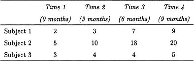
Table 5.1
Data for a Simple Longitudinal Study
The parameters of the model and, consequently, the parameters that must be estimated are the fixed effects (β), the random-effect variances and covariances (G), and the error variances and covariances (R). The random effects (u) are not model parameters and often are not of interest to researchers because they are specific to particular subjects (although the random effects can be predicted and the predictions could be included in hypotheses and tested).
A Simple Example
To illustrate the mixed model, we consider a very simple example in which infants are assessed in their perceptual skills at 0, 3, 6, and 9 months of age, and we are interested in their rate of growth over this time period. The data are presented in Table 5.1. In developing a model, we assume that perceptual skills develop linearly across time, but that this relationship might vary from person to person.
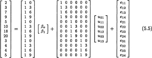
First we substitute into the prediction equation for the mixed model, y = Xβ + Zu + e, the appropriate values:
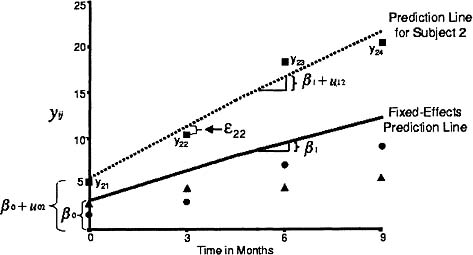
Figure 5.1: Graph for simple example illustrating fixed and random effects.
The design matrix X and the fixed-effects coefficients β are defined in exactly the same manner as they are in the general linear model, and β0 and β1 have comparable meaning. According to a mixed model analysis, β0 = 3.300 and β1 = .933; the intercept, β0, represents the mean perceptual skill for all children at 0 months of age, whereas the slope, β1, represents the mean perceptual skill for each month of age. The fixed-effects (or population-mean) prediction line is shown in Figure 5.1.
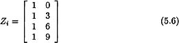
Next we examine the random-effects component, Zu. Along the diagonal of the random-effects design matrix Z are the design matrices for the individual subjects, and these design matrices are the same for all subjects:
The random coefficients in u, u0i and u1i, represent residual intercepts and slopes, respectively. For this model, the first two observations for subject 1 can be written algebraically as:
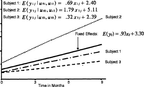
Figure 5.2: Graph for simple example illustrating the variability of the prediction lines for individual subjects around the line for the population.
![]()
and
![]()
As shown in Figure 5.1, the prediction line for subject 2 has an intercept of β0 + u02 and a slope of 1 + u12, whereas the prediction line for the population has an intercept of β0 and a slope of β1. Accordingly, the residual intercept, u02, is the difference between the intercept for subject 2 and the intercept for the population prediction line. Similarly, the residual slope for subject 2, u12, is the difference between the slope for subject 2 and the slope for the population prediction line. Although typically we would not estimate the random coefficients, we did so for illustrative purposes. The residual intercepts are -.900, 1.806, and -.907 for subjects 1, 2, and 3, respectively, whereas the residual slopes are -.241, .852, and -.612 for the same three subjects. Given the fixed-effects intercept and slope are 3.300 and .933, respectively, the intercepts and slopes are 2.400 (3.300 .900) and .692 (.933 - .241) for subject 1, 5.106 (3.300 + 1.806) and 1.785 (.933 + .852) for subject 2, and 4.393 (3.300 - .907) and .321 (.933 - .612), for subject 3, respectively. The differences in the intercepts and slopes for subjects are graphically displayed in Figure 5.2.
The model parameters in G are the variances and covariances among elements of the subject-specific vectors imbedded in the vector u. In this example, we included not only the variances for the residual intercepts and residual slopes but also the covariances between the residual intercepts and slopes. Given that no distinctions were made among subjects, we assumed homogeneity of variances and covariance of the random effects across subjects. Under these conditions, the covariance matrix Gi is the same for all subjects,
![]()
where ![]() is the variance in intercepts between subjects,
is the variance in intercepts between subjects, ![]() is the variance in slopes between subjects, and
is the variance in slopes between subjects, and ![]() is the covariance between the intercepts and slopes. The structure of G is:
is the covariance between the intercepts and slopes. The structure of G is:
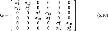
For our example, ![]() ,
, ![]() , and σ12 were estimated to be 2.707, .591, and 1.130, respectively. The magnitudes of these variances and covariance are consistent with the values for the estimated residual intercepts and slopes. For example, the estimated residual intercepts and slopes appear strongly positively related, and the correlation between them based on variances and covariances in G is
, and σ12 were estimated to be 2.707, .591, and 1.130, respectively. The magnitudes of these variances and covariance are consistent with the values for the estimated residual intercepts and slopes. For example, the estimated residual intercepts and slopes appear strongly positively related, and the correlation between them based on variances and covariances in G is ![]() .
.
As illustrated in Figure 5.1, a within-subject error, eij, represents the deviation of an observation at time j for subject i from that subject’s individual prediction line. These deviations may represent departures of the subject’s growth curve from linearity, measurement errors, or a combination of both. The variance of these errors is a model parameter and was estimated in our example to be 1.333. Given we do not hypothesize any covariance among the within-subject errors and assume homogeneity of these errors across all subjects, R is a 12 × 12 matrix with 1.333 along its diagonal. The covariance matrix among the dependent variable scores is a function of the random-effects design matrix, the covariance matrix among the random effects, and the covariance matrix among the within-subject errors, that is, ![]() . In our example, we estimate V as
. In our example, we estimate V as
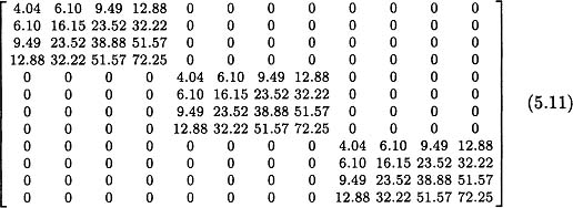
V indicates that variances increase with time and correlations are larger if they are between later observations. These results are consistent with the data as displayed in Figures 5.1 and 5.2 that show a greater divergence in the Y scores from the line for the fixed effects at later observations.
ESTIMATION AND STATISTICAL INFERENCE
Estimation is more complicated in the mixed model than in the general linear model in that, not only are the fixed-effects parameters in β unknown, but also the variance and covariance parameters in G and R must be estimated. Unlike the general linear model, they generally cannot be estimated independently of the fixed-effects parameters. As noted by Littell et al. (1996), the appropriate method for estimating the components of β is no longer ordinary least squares but rather generalized least squares using the inverse of V as the weight matrix. However, the elements of V are seldom known. Consequently, estimation is generally based on likelihood-based methods as described in detail by Laird and Ware (1982), Harville (1977), and Jennrich and Schluchter (1986) among others, assuming that u and e are normally distributed.
Likelihood-based methods yield distinct estimating equations for the fixed-effects parameters and variance components, with the fixed-effects estimating equations requiring estimates of the variance components and estimating equations for the variance components requiring estimates of the fixed effects. Consequently, the overall estimation procedures require iteration between the fixed-effects equations and variance components equations to reach a final solution. First, we consider methods to obtain variance component estimating equations followed by a discussion of the fixed-effects estimating equations.
The two principal methods for estimating variance components are maximum likelihood (ML) and restricted (or residual) maximum likelihood (REML). Under the assumption of normality for both the random effects and the error terms, the likelihood function for the mixed model for all subjects combined has the form (Hocking, 1985):
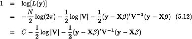
in which the variables in the model are defined previously. Standard maximization procedures can be used to derive a set of nonlinear estimating equations for the components of V, but these equations generally involve the elements of β.
Patterson and Thompson (1971) proposed REML as an alternative method for estimating covariance parameters. This procedure relies on using the error space of the fixed-effects design matrix to estimate the covariance parameters. The justification for the REML suggested by Patterson and Thompson (1971) relies on modifying the ML procedure via factorization of the likelihood function. Conceptually, this process involves partitioning the data space into two orthogonal components: the estimation space, defined as the column space of X, and the orthogonal complement of the estimation space, the error space. Mathematically, one can project the data vector onto the error space and estimate the variance components from this error space independently of the fixed effects. This procedure accounts for the loss of degrees of freedom needed to estimate the fixed effects and is analogous to using the mean square error to estimate σ2 in classic ANOVA. Harville (1974) offers a justification of this procedure from a Bayesian framework and presents a convenient form of a likelihood function that can be used to obtain REML estimates:
![]()
Estimates for the components of V can be obtained by maximizing this function, again to obtain a set of nonlinear estimating equations dependent on the elements of β. The SAS procedure MIXED can be used to develop either ML or REML estimates, with REML estimates generally preferred unless the data sets are quite large.
Conditional upon V being known, either ML methods or general least-squares methods can be used to derive the following set of estimating equations for the fixed effects parameters:
![]()
To obtain estimates for β, the estimates of the variance components from the ML or REML estimation procedure are used in the previous estimating equation. Either the ML or REML estimation can be implemented with the SAS MIXED procedure.
Statistical inference in the mixed model is generally concerned with tests concerning the fixed effects that can be formulated in terms of secondary parameters that are linear combinations of the fixed-effects parameters in β. More precisely, c secondary parameters are in a column vector θ, with θ = C1β − θ0, where C1 is c × q matrix that contains the coefficients for the c linear combinations of fixed-effects parameters and θ0 is a c × 1 vector consisting of constants, in practice almost always zeros. The hypotheses of interest are of the form H0: θ = 0 versus Ha: θ ≠ 0. Three types of test statistics have been proposed for testing hypotheses of this type: likelihood ratio tests, Wald tests, and approximate F tests (Littell et al., 1996). Simulation studies indicate that Wald tests tend to be overly liberal, possibly by as much as a factor of 2 for mixed models (Woolson & Leeper, 1980), and that likelihood ratio tests also tend to be overly liberal (Andrade & Helms, 1986). In contrast, simulation studies by McCarroll and Helms (1987) suggested that an approximate F-test provides reasonable Type I error protection. Consequently, we recommend that the approximate F test, as described by Littell et al. be used. Using hypothesis tests as defined previously, the approximate F-test has the form:
![]()
where V = σ2Γ. The numerator degrees of freedom for the test are generally accepted to be the rank of C1, but as discussed in the section on modeling issues, no general consensus has been reached as to the best choice of denominator degrees of freedom for the test. The test statistic is implemented in the SAS MIXED procedure.
ISSUES IN APPLYING MIXED MODELS TO LONGITUDINAL DATA
Statistical modeling provides best results if researchers have a clear understanding of the characteristics and structure of their data and implement a well-formulated analysis strategy in response to explicitly defined research questions. Issues such as how measurements are made, how data are collected, bias in subject selection, and distributional properties of outcomes that are important in constructing a statistical model using classic regression or ANOVA techniques are also important for analysis of repeated measures data with mixed models. Investigators must address these issues to obtain reliable results from mixed model analyses; however, we will focus on issues that are unique to mixed models and repeated measures data.
Longitudinal data with multiple observations on the same subject are inherently more complicated statistically than independent observations from different subjects. Two interrelated factors that contribute to this complexity are that observations on the same subject are correlated and that the data contain both between-subject and within-subject information. The linear mixed model provides great flexibility for handling these added complexities, but the flexibility comes with a price, as investigators must decide among diverse options in selecting a model structure. All statistical models involve distributional assumptions about the mean and variance structures of the data, but modelers tend to focus on the mean or expected value component given the limited choices among the variance components for most statistical procedures. In contrast, application of linear mixed models to longitudinal data requires the modeler to address both the expected value (fixed effects) and the variance (or random effects) components explicitly.
Recall that the mathematical formulation of the mixed model is:
![]()
with β representing the fixed effects and both u and e representing random effects, although the actual parameters of the random effects are associated with the covariance matrices G and R of u and e, respectively. Hence, in developing the model, the researcher must specify the parameters that are included in the vector β, generally through the specification of the design matrix X, and the structure of G and R. Specifying the structure of the individual parameters in the fixed effects vector β is a bit more complicated in the mixed model with longitudinal data than in the classic linear model for independent data in that the investigator must determine how to handle between-subject and within-subject information. The paragraphs that follow first discuss some of the options available for characterizing the variance components of the model. Then, issues related to handling within-subject and between-subject information in the fixed-effects component of the model are discussed.
Random-Effects Components of the Mixed Model
The variance-covariance components in the random-effects components of the linear mixed model can be partitioned into two types—those associated with u, the between-subject variance-covariance components, and those associated with e, the within-subject variance-covariance components. The ways in which the variability in the outcome can be partitioned between these two components and the structures that can be used for G and R are quite diverse and are limited only by the capabilities of the software and the insight of the researcher. Because the number of structures that one might encounter is so wide ranging, we describe only some of the more widely used ones in this chapter.
Between-Subjects Random Effects (G Matrix).
One of the simpler models that falls within the framework of the mixed model is the classic univariate approach to repeated measures analysis of variance. In this model, the variance is partitioned into two components, a between-subject variance component (![]() ) and a within-subject variance component (
) and a within-subject variance component (![]() ). We start with this relatively simple model and then generalize to models with more complex random-effects components.
). We start with this relatively simple model and then generalize to models with more complex random-effects components.
Consider a simple repeated measures experiment with 2 groups representing 2 subpopulations, 3 subjects per group, and 3 replications, for a total of 18 observations. The fixed-effects component of the model can be modeled in the usual way and is not of concern here. To obtain the appropriate structure for the variance components, which is a compound symmetric V matrix under the usual assumptions of repeated measures ANOVA, we construct a block diagonal Z matrix with 18 rows and 6 columns as shown in Figure 5.3. The G matrix is simply ![]() * I6 (where IN is an N × N identity matrix), and the R matrix is
* I6 (where IN is an N × N identity matrix), and the R matrix is ![]() * I18. Under these conditions, V is compound symmetric, as can be shown by substituting into the following equation, V = ZGZ′ + R. Conceptually, this classic model can be viewed as a model in which the subjects are random effects (hence the blocks in the Z matrix), with each subject having a mean score (or intercept) that deviates from the mean for the subject’s subpopulation. The residual intercepts are assumed to be normally distributed with a mean of 0 and a variance of
* I18. Under these conditions, V is compound symmetric, as can be shown by substituting into the following equation, V = ZGZ′ + R. Conceptually, this classic model can be viewed as a model in which the subjects are random effects (hence the blocks in the Z matrix), with each subject having a mean score (or intercept) that deviates from the mean for the subject’s subpopulation. The residual intercepts are assumed to be normally distributed with a mean of 0 and a variance of ![]() .
.
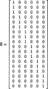
Figure 5.3: Random effects design matrix for repeated measures model.
Now let’s assume that we want to apply a more complicated model that allows for different linear growth curves for different subpopulations. The data are from a study like the one just described (3 subjects in each of 2 groups, with each subject measured at 3 times), except the three times each subject is measured differs across subjects. Ignoring the fixed-effects component of the model, the random-effects component can be viewed as an expansion of the one for the traditional repeated measures ANOVA model: Subjects are still random, but each subject deviates from the subpopulation average behavior not only in location but also in slope. Because different subjects are measured at different times in this study, they are likely to show differential slopes assuming growth is occurring, even if in theory growth is uniform over a fixed period of time for all subjects. The appropriate Z matrix for this model is shown in Figure 5.4. Note the block diagonal structure of this matrix with each block of two columns representing a single subject. For each subject, the structure in Z is constructed in essentially the same way that a design matrix is structured in a univariate linear model. Within each block, the first column is a column of 1’s associated with the subject-specific deviations from the population average (fixed-effect) intercept, and the second column contains the times of each observation for a specific subject. These times are associated with the subject-specific deviations from the population average (fixed-effect) slope. Assume that the R matrix for this model is the same as the earlier model, that is, ![]() * I18. We can begin to see the flexibility of the mixed model by assessing how to model the G matrix. The matrix must have greater structure than the traditional repeated measures model because we must now consider between-subject variability in slopes as well as intercepts. In addition, we must consider whether the subject-specific deviations in intercept and slope are independent or correlated with each other. We could allow the variances for residual intercepts and slopes to differ or constrain them to be equal; however, we would have difficulty developing a research scenario that would justify constraining these variances to be equal in the context of our example. To demonstrate the flexibility of the mixed model, we also introduce the possibility that the variance components for the intercept and the slope differ between groups.
* I18. We can begin to see the flexibility of the mixed model by assessing how to model the G matrix. The matrix must have greater structure than the traditional repeated measures model because we must now consider between-subject variability in slopes as well as intercepts. In addition, we must consider whether the subject-specific deviations in intercept and slope are independent or correlated with each other. We could allow the variances for residual intercepts and slopes to differ or constrain them to be equal; however, we would have difficulty developing a research scenario that would justify constraining these variances to be equal in the context of our example. To demonstrate the flexibility of the mixed model, we also introduce the possibility that the variance components for the intercept and the slope differ between groups.
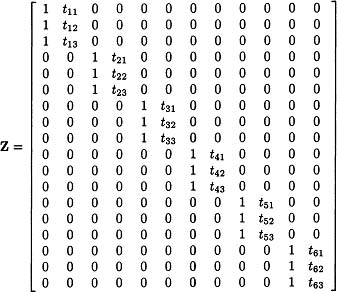
Figure 5.4: Random effects design matrix for random slope model.
Figures 5.5-5.7 outline three different G matrices that might be specified based on these considerations. Figure 5.5 presents a covariance matrix for the random effects in which the residual intercepts and slopes can have different variances, the covariance between the residual intercepts and slopes is constrained to 0, and the variances are constrained to be equal between the two groups. Figure 5.6 presents a covariance matrix for the random effects in which the residual intercepts and slopes can have difference variances, the covariance between the residual intercepts and slopes is constrained to 0, but the variance components are allowed to differ between the two groups. Finally, Figure 5.7 presents a covariance matrix for the random effects in which the residual intercepts and slopes can have difference variances, the covariance between the intercept and slope is allowed to be nonzero, and the variance and covariance parameters are constrained to be equal between the two groups. We address how we should choose among these different structures in a later section about modeling strategy.
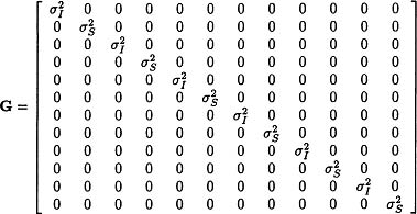
Figure 5.5: Alternative form of G matrix for random slopes model.
Within-Subjects Random Effects Matrix.
The previous discussion examined alternative approaches to modeling the between-subject random-effects component with little attention to the within subject variance component. In all cases, we assumed that the R matrix would have a very simple structure, that is, ![]() * I. An alternative strategy for modeling is to focus on the R rather than the G matrix. As discussed earlier, the R matrix characterizes the variance structure for the within-subject residuals after the model accounts for the population or fixed effects and the subject-specific random-effects deviations from those fixed effects. One approach to modeling longitudinal data is to choose the Z matrix to be 0 and to model all of the variation from the fixed effects with the R matrix. Even within this relatively general approach, the assumptions described earlier place some constraints on the structure of the R matrix. First, subjects are generally assumed to be independent, forcing the structure of the matrix to be block diagonal with each subject representing a block. Second, at least some level of homoscedasticity across subjects is assumed, constraining the variance components to be the same in each block. If a study contains multiple subpopulations, this constraint may be relaxed somewhat to allow different variance components for different subpopulations, but within subpopulations, subjects are assumed to have the same variance-covariance components.
* I. An alternative strategy for modeling is to focus on the R rather than the G matrix. As discussed earlier, the R matrix characterizes the variance structure for the within-subject residuals after the model accounts for the population or fixed effects and the subject-specific random-effects deviations from those fixed effects. One approach to modeling longitudinal data is to choose the Z matrix to be 0 and to model all of the variation from the fixed effects with the R matrix. Even within this relatively general approach, the assumptions described earlier place some constraints on the structure of the R matrix. First, subjects are generally assumed to be independent, forcing the structure of the matrix to be block diagonal with each subject representing a block. Second, at least some level of homoscedasticity across subjects is assumed, constraining the variance components to be the same in each block. If a study contains multiple subpopulations, this constraint may be relaxed somewhat to allow different variance components for different subpopulations, but within subpopulations, subjects are assumed to have the same variance-covariance components.
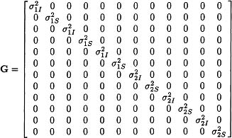
Figure 5.6: Alternative form of G matrix for random slopes model.
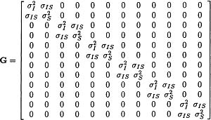
Figure 5.7: Alternative form of G matrix for random slopes model.
![]()
Figure 5.8: Alternative structure for the R matrix. Unstructured.
Again, consider the study with three subjects in each of two groups, with measurements at three time points for each subject. Assume that all deviations from the fixed effects are to be modeled in the R matrix. Figures 5.8-5.13 present six common variance-covariance structures that are used to model the within-subject variability. Each matrix represents a block for a single subject (Ri) from the block-diagonal R matrix. Figure 5.8 represents the most flexible structure, the unstructured covariance matrix. This matrix allows variances to differ at all time points and a different covariance between any pair of time points and requires estimation of 6 variance-covariance parameters. In contrast to Figure 5.8, Figure 5.9 represents the most constrained structure, with variances at all time points assumed to be equal and covariances between all time points assumed to be 0. This structure implies that the observations on the same individual are independent of each other and is often unrealistic for longitudinal studies, unless subject effects are addressed in the G matrix. The structure in Figure 5.10 expands the structure from 5.9 to allow different variances at the three time points. Again, unless subject effects are addressed in the G matrix, this model is likely to be unrealistic for longitudinal studies because it does not permit dependence among observations for subject. Figure 5.11 represents a compound symmetric structure with equal variances at each time point, and correlations across time assumed to be equal (i.e., the correlation between subject i’s observations at times 1 and 2 is equivalent to the correlation between the observations at times 1 and 3). The resultant V matrix differs slightly from the one for the repeated measures ANOVA model in that the correlation across time may be negative or positive in Figure 5.11, but is constrained to be non-negative with the repeated measures ANOVA structure. The matrix in Figure 5.12 is a slight expansion from that in 5.11 in that variances are allowed to differ at different time points, but correlations between time points are constrained to be equal. Finally, Figure 5.13 represents a first-order autoregressive model in which the covariances decrease between observations that are further apart.
The variance-covariance structures depicted in Figures 5.8 through Figure 5.13 vary greatly. As few as one variance component is estimated for Figure 5.9, whereas as many as six variance and covariance components are estimated for Figure 5.8. These structures represent only a few of the types of structures that might be considered. Each of these structures could obviously be extended to allow different variance-covariance components for different subpopulations. However, the complexity of the structure that can be developed is often limited by the amount of data available for the study.
Figure 5.9: Alternative structure for the R matrix. Independence.
![]()
Figure 5.10: Alternative structure for the R matrix. Unequal time variance.
![]()
Figure 5.11: Alternative structure for the R matrix. Compound symmetric.
![]()
Figure 5.12: Alternative structure for the R matrix. Heterogeneous compound symmetric.
![]()
Figure 5.13: Alternative structure for the R matrix. First-order autoregressive.
As suggested by the previous paragraphs, the combination of G and R matrices provide great flexibility in modeling variance-covariance structures. The model provides some redundancy in that the “same” model can be generated by partitioning variance components differently across the two matrices. For example, specifying a single between-subject variance component in G with an identity matrix for R results in the same structure as specifying no random components and a compound symmetric R matrix. Because these alternative formulations of the model produce the same results, the researcher selection of one over the other has no practical differences. Wolfinger (1993) suggests that random effects are more suited to modeling correlation among a large number of observations whereas, covariance modeling in R is more local. Typically our approach is to select an overall structure for V and partition the variance components between G and R in a way that makes the variances and covariances most interpretable within the study design.
Fixed-Effects Component of the Mixed Model
Generally, the strategies for developing the fixed-effects components of the model are similar to those used to develop linear models when the observations are independent. However, one additional issue that must be addressed is the potential confounding of within-subject and between-subject relationships in the computation of fixed-effects estimates (Jacobs et al., 1999; Kreft & de Leeuw, 1998). Consider a study in which longitudinal data are collected at grades 1 through 6 and the primary question is whether student achievement in mathematics and teacher expertise in mathematics covary as students progress through these six grades. If a model is constructed that simply predicts student achievement from teacher expertise, the β1 estimate associated with student achievement is based on both the within-subject and the between-subject relationships between these two variables. This estimate is interpretable only if the within-subject and the between-subject relationships are the same. In other words, to use this estimate, the observations within and between subjects are assumed to be exchangeable, that is, the relationship between achievement and expertise for a particular student at two time points (within-subject) is assumed to be the same as the relationship between achievement and expertise for two different students at the same time point (between-subject relationship).
This assumption is not likely to be viable in most behavioral science applications. For these cases, the fixed-effects component of the model should be constructed in such a way as to partition the relationship into between-subject and within-subject estimates. As described by both Kreft and de Leeuw (1998) and Jacobs et al. (1999), this partitioning can be accomplished by including in X (i.e, the fixed-effects design matrix) the mean predictor scores for subjects (subject-specific mean) and the deviations of the predictor scores around their subject-specific means. In our example, a subject-specific mean is computed by averaging the teacher expertise for a student across grades for that subject, whereas a deviation score is a subject’s teacher expertise score for a grade minus the student-specific mean teacher expertise score for that subject. The coefficient for the mean is then interpreted as a between-subject effect, and the coefficient for the deviation score is interpreted as a within-subject effect.
IMPLEMENTING MIXED MODELS USING SAS PROC MIXED
PROC MIXED© is implemented through a series of commands or statements. Many models can be fit using only five statements: PROC MIXED, CLASS, MODEL, RANDOM, and REPEATED. Each of these statements has a distinct purpose that is consistent with the mathematical structure of the mixed model described earlier. We briefly describe each of the statements.
PROC MIXED
This statement initiates the algorithm and identifies the source of data to be used in the analysis. The METHOD= option allows the investigator to specify the method used to estimate parameters (e.g., REML and ML).
CLASS
This statement identifies predictors as classification variables and creates dummy variables for these classification variables in the X and Z matrices.
The MODEL statement in PROC MIXED is similar to the model statement in PROC GLM and establishes the structure of the fixed-effects component (Xβ). The fixed-effect predictors may include classification or continuous variables and includes the intercept by default. PROC MIXED uses a less-than-full-rank parameterization for classification variables, which is identical to the one used in PROC GLM (Green, Marquis, Hershberger, Thompson, & McCollam, 1999).
RANDOM
This statement specifies the structure of the G matrix by listing the random-effects predictors that are to be included in the Z matrix. Unlike the MODEL statement, an intercept is not included in the RANDOM statement by default and must be specified (INT) if required. The key options on the RANDOM statement are SUBJECT=, which defines the subjects in the data set needed to create the block diagonal structure in the Z matrix; TYPE=, which specifies the type of structure in the G matrix; and GROUP=, which allows heterogeneity in variance components across sub-populations.
REPEATED
It specifies the structure of the R matrix. If no REPEATED statement is used, the structure of R is assumed to be σ2I. Key options on the REPEATED statement are SUBJECT=, which defines the subjects in the data set needed to create the block diagonal structure in the R matrix, TYPE=, which specifies the type of structure in the R matrix; and GROUP=, which allows heterogeneity in variance components across subpopulations.
The goal for this section was to show that the syntax for PROC MIXED was developed to reflect the various parts of the mixed model. Other sources are required to understand how to structure the data set and how to write the code to conduct analyses using PROC MIXED. Readers are encouraged to read the SAS documentation (SAS, 1997) on PROC MIXED and consult excellent references by Littell et al. (1996) and Singer (1998).
A FOUR-STEP MODELING STRATEGY FOR BUILDING AND REFINING MIXED MODELS
As with any model-based data analysis, investigators must clearly define the research questions that the model is designed to answer. If the questions are not well defined, the likelihood of the results yielding unambiguous answers is negligible. Although research questions may address parameters associated with the random-effects part of the model, most research questions are answered by the fixed-effects part. In constructing the design matrix for the fixed-effects component, investigators should include not only the predictors that directly address the research questions but also possible confounding variables and moderator variables. In addition, if there are time-varying predictors, decisions must be made concerning how to include them in the model so as to differentiate or not differentiate between the between-subject and within-subject effects for them.
If the random effects or fixed effects are misspecified, the hypothesis tests for these effects are biased. Accordingly, investigators must use some modeling process that requires them to evaluate what fixed-effects parameters are important to include in the model given the random effects parameters are correctly specified and to assess what random-effects parameters are important to include in the model given the fixed-effects parameters are specified correctly. No single approach yields the ideal modeling strategy because of the complexity of model, and different modeling strategies are often necessary for different types of analyses. Nevertheless, we suggest a modeling strategy that provides a platform for investigators who are novice users of mixed models that can be adapted with experience in analyzing data with mixed models. Multiple replications of a modeling strategy such as the one described subsequently are often needed to address research questions posed by a study.
Step 1. Review past literature in the substantive area and conduct descriptive analyses on the sample data to formulate an understanding of the data for the development of the initial mixed model.
By reviewing theories explaining the phenomenon of interest and relevant empirical literature, investigators should be in a better position to describe what they should find when they analyze their data. For example, an investigator might conclude from a literature review that growth on an outcome variable should generally show marked improvement over the initial observations but then show slower improvement. In addition, the pattern of growth should vary over individuals. The first conclusion would help an investigator formulate the fixed-effects component of the model, whereas the second conclusion would aid in the development of the random-effects component of the model.
Investigators should gain further insights into the probable outcome of their analyses by computing descriptive statistics and creating graphs. For example, investigators could make judgments about the fixed-effects components by examining the box-plots on the outcome variable for each occasion as well as their means and standard deviations for occasions. Investigators could make decisions about both fixed-effects and random-effects components by developing plots of the subject-specific empirical growth curves (sometimes called spaghetti plots because of their appearance) that show the changes over time for individual subjects in a study. Depending on the number of subjects in the study, a single plot can contain the growth curves for all subjects (for a small number of subjects) or only a random selection of subjects if the number is so extensive that patterns are obliterated by the volume of data.
Literature is developing that should help investigators with this step. Christensen, Pearson, and Johnson (1992) have extended graphical and diagnostic techniques developed for the general linear model to mixed models, and these techniques are often useful for model development. Also, Grady and Helms (1995) describe some ad hoc techniques useful for selecting an appropriate structure for the R matrix.
Step 2. Formulate an initial mixed model and evaluate the fixed-effects parameters.
At this step, select a relatively simple structure for the random-effects component that does not conflict with the conclusions drawn from Step 1. Next choose a fixed-effects component with a relatively large number of parameters that is still consistent with the conclusions from Step 1. Then use a data-driven strategy to generate a more parsimonious fixed-effect component by eliminating predictors that do not appear to be related to the outcome. However, regardless of the results, some parameters are likely to be retained in the model to address the research questions appropriately. Use the approximate F-test to evaluate predictors (see Equation 5.6).
Step 3. Evaluate the structure of the random-effects component, while the fixed-effects component includes the predictors that appeared important on the basis of Step 2.
Using the fixed-effects structure from Step 2, model the covariance structure, starting with the most feasible complex structure that is consistent with the conclusions from Step 1. Next use a data-driven strategy to move toward a simpler structure. For nested models with no change in fixed effects, a likelihood ratio test based on differences in REML likelihoods can be used to discriminate between models. For models that are not nested, likelihood-based selection criteria, such as Akaike’s and Schwarz’s criteria, have been adapted for mixed models, but information about their performance in small to moderate samples is limited (Bozdogan, 1987; Wolfinger, 1993).
Step 4. Fine tune the fixed-effects structure and random-effects covariance structure.
Accuracy of tests of the fixed effects depends on whether the random-effects component is correctly specified, and accuracy of tests of the random effects depends on whether the fixed-effects component is correctly specified. Consequently, the fixed-effects component of the model could be re-examined next, whereas the random-effects component is specified based on the results of Step 3. Potentially, this process of alternately assessing random-effects and fixed-effects components of the model continues until no changes in the model structure are necessary.
EXAMPLE MIXED MODEL ANALYSIS
Schumacher et al. (1999) conducted a longitudinal study that investigated the relative effectiveness of two treatment programs designed to reduce addiction in homeless individuals with cocaine addiction. Each participant in the study was assigned to one of two treatment groups and assessed on multiple measures prior to treatment and at 2, 6, and 12 months during treatment. One treatment group received immediate abstinent-contingent housing followed by abstinent-contingent housing, work therapy, and aftercare (DT+), whereas the other group received only work therapy and aftercare (DT).
The hypotheses for our analyses focus on the effect of treatment on drug addiction and the relationship between depression and drug addiction. Drug addiction was measured by the Addiction Severity Index (ASI), which yields aggregate scores ranging from 0 to 100, whereas depression was measured by the Beck Depression Inventory (BDI), which produces total scores ranging from 0 to 63, with a score of 16 used as the cutoff for labeling individuals as depressed. Our analyses included 141 subjects, 69 from the DT group and 72 from the DT+ group. The number of subjects with scores on the ASI varied across the observations at 2, 6, and 12 months postintervention: 48, 49, and 43, respectively, for the DT subjects and 62, 61, and 57 for the DT+ subjects. Retention in the study was greater for DT+ than for DT subjects, but for simplicity of presentation we conducted our analyses assuming observations were missing at random.
Step 1
We examined a series of issues in Step 1. Because both the ASI and the BDI measures were assessed over time, we had to consider whether the relationship between them is the same within a subject as it is between subjects. Equality of the within-subject and the between-subject relationships appeared conceptually untenable. Accordingly, we created two predictors to examine the relationships separately: a between-subject BDI predictor and a within-subject BDI predictor. Scores on the between-subject BDI predictor were computed as mean BDI across time for each subject, and scores on the within-subject BDI predictor were calculated as deviations between a BDI score for a particular time and the mean BDI across time for each subject.
Also at Step 1, we examined graphs to assess the within-subject relationship between depression and addiction across time for each subject as well as graphs to evaluate the between-subject relationship between depression and addiction across subjects at each time. For both sets of graphs, the variables appeared to be monotonically related with no readily apparent nonlinear effects. The level of addiction and magnitude of linear slope seemed to vary across subjects, which would suggest the possibility of nonzero variances for both of these terms. We decided not to consider nonlinear relationships between the BDI and ASI scores for three reasons: (a) graphical results failed to support nonlinear relationships; (b) no theoretical rationale could be provided for these relationships, and (c) an insufficient number of time points (at most three observations) were collected to examine these nonlinear relationships reliably.
We visually examined the plots also to evaluate whether the model should include interactions between depression and treatment. Although the plots showed no apparent differences in relationships between drug addiction and depression as a function of treatment, both between-subject and within-subject interactions were considered for inclusion in the model because of the difficulty in detecting interactions in the complex graphical displays and because theoretical rationales could be provided for their existence. Finally, general practice in the addiction literature is to control for baseline level of addiction in reporting results; consequently, we included the baseline drug addiction score in all models.
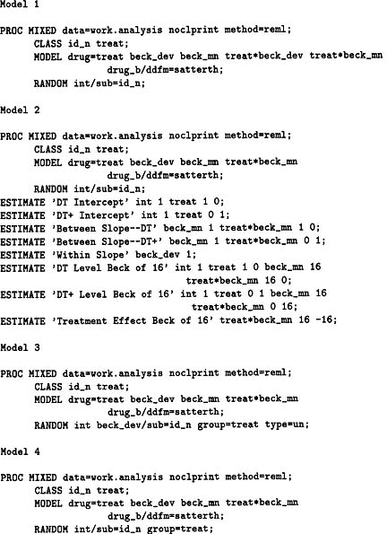
Step 2
At Step 2, we developed an initial model with a relatively simple structure for the random-effects component and a relatively complex fixed-effects structure that was consistent with the conclusions from Step 1. The random-effect component included only a random intercept or location effect in G and a common residual variance in R. In this case, both G and R are diagonal matrices, with G having the between-subject variance and R having the within-subject variance on the diagonal. The dimension of G is the number of subjects in the study (141) and the dimension of R is the total number of observations at all three time points (320). Letting tx = treatment (0 = DT and 1 = DT+), beck_mn = between-subject BDI predictor, beck_dev = within- subject BDI predictor, id_n = subject ID, drug_b = baseline ASI, and drug = ASI at a particular time, the key SAS code for Model 1 is shown in Table 5.2. This code creates a less-than-full-rank fixed-effects design matrix (X) with 10 columns: a column for the intercept, 2 columns for the treatment effect, 1 column for the between-subject BDI predictor, 1 column for the within- subject BDI predictor, 2 columns for the interaction of treatment with the between-subjects BDI predictor, 2 columns for the interaction of treatment with the within-subjects BDI predictor, and 1 column for the baseline ASI predictor.
The model was fit with REML estimation techniques. Results from this model (Model 1) were examined with a primary emphasis on simplifying the fixed effects using approximate F tests. The results (not shown) suggested that treatment-specific slopes were not needed for the within-subject relationship between BDI and ASI (p = 0.51 for the treatment by beck_dev interaction). Results also suggested that the treatment intercept did not differ by group (p = 0.46) and the baseline ASI was unimportant (p = 0.23). However, these latter parameters were retained in the model; the first source addresses one of the research hypotheses and the second source is required to minimize confounding.
A revised model (Model 2) was fit next; the SAS code for this model is shown in Table 5.2. Model 2 was identical to Model 1 except the interaction of treatment with the within-subjects BDI predictor was eliminated based on the results of Model 1. Table 5.3 gives the SAS output for Model 2 from the PROC MIXED analysis. (Ignore for the moment the ESTIMATE statement and its associated results.) First, the iteration history summary indicates that the estimation procedure converged. The covariance parameter estimates show that the between-subject variance associated with the intercept (INTERCEPT) is approximately 14, whereas the within- subject residual variance (Residual) is approximately 73. Of primary interest are the tests of fixed effects, which indicate that the ASI scores are related to depression both longitudinally (p < .0001 for the BECK_DEV effect) and cross-sectionally (p <0.001 for BECK_MN), and the cross- sectional effect differs by treatment group (p = 0.005 for TREAT*BECK_MN). Because we wish to retain the treatment intercept effect and the baseline ASI in the model regardless of the significance test results, no further simplification of the fixed-effects component of the model is required. In other words, Model 2 represents a final model for Step 2.
Table 5.2
SAS Code for Example Models of Drug Addiction
In Step 3, we consider models with alternative random-effects components while maintaining the same fixed-effects component based on the results of Step 2. We initially considered two alternative covariance structures. For both structures, we included variances for both intercepts and slopes and a covariance between the intercept and slope. For Model 3a (see Table 5.2 for SAS code) we allowed separate covariance parameters for the treatment groups (by using the GROUP = tx option in the RANDOM statement), whereas for Model 3b we constrained the variance and covariance parameters to be the same for the two treatment groups. For both of these models, R was the same diagonal matrix of dimension 320 used earlier. For both models, the G matrix is block diagonal with blocks of dimension 2 with each block having a between-subject variance in intercept deviations, a between-subject variance in slope deviations, and the covariance between intercept and slope deviations. The structure of the two models is the same, but one model allows for six variance components and the second model constrains the number of components to three. Both models failed to converge, but the small estimates for the slope variance on the last iteration of each model suggested that the models might be overspecified. Convergence problems with the slope in the model may also have been related to the small number of observations per subject (3) and the limited variability in BDI scores for some subjects. One final model, Model 4, was fit (see Table 5.3 for SAS code) that allowed for a different variance for the intercepts for each treatment group but constrained the variance for the slopes to be zero. Because Model 2 is nested within Model 4, we compared the REML likelihoods, with the -2 REML log likelihoods being 2295.42 for Model 2 (see Table 5.3) and 2295.38 for Model 4 (result not shown). The likelihood ratio test for comparing the two models is the difference in these two values. The resulting χ2 = 0.04 with 1 df suggests that the simpler Model 2 is preferred. Because Model 2 was selected in Step 2 as the final model, the fitting process is complete, making Step 4 unnecessary.
Table 5.3
Illustrative PROC MIXED Output Based on Model 2
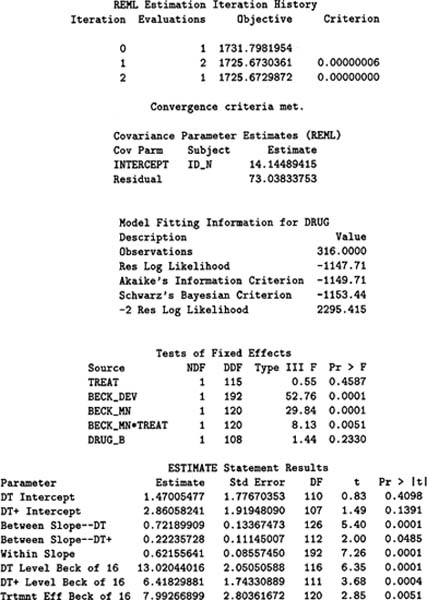
The results from the ESTIMATE statement used in Model 2 are now helpful in interpreting the final model. The ESTIMATE statement generates an estimate of a linear combination of the fixed-effects parameters, the standard error of this linear combination, and the test statistic and p value for the test that the true population value for this linear combination is 0. The results indicate that a within-subject change of 10 units on the BDI results in a change of 6 units on the ASI scale, whereas a difference of 10 units on the BDI results in a difference of 7.2 units in the DT group and a difference of 2.2 units in the DT+ group. At a BDI score of 0, the DT and DT+ groups show a nonsignificant difference in the drug addiction score of 1.4 units, whereas at a Beck score of 16 (a level defined as signifying a depressed state) the difference in mean between DT and DT+ groups is about 8 units, with the DT+ group having on the average lower scores on the ASI than DT group (p = 0.005). The results suggest that addiction level is related to depression and that the abstinent-contingent housing component has a greater effect in reducing addiction in more depressed individuals. Potentially, additional analyses could be conducted to address the research questions. For example, time could be introduced into the analyses as a covariate to assess if the relationship between the BDI and ASI maintains itself controlling for time. To address this question, we would have to initiate the modeling strategy again but now include not only the predictors that we previously used but also time and higher-order interaction terms with time.
CONCLUSION
We believe that the mixed model has wide applicability in the analyses of repeated measures data collected by behavioral science researchers. We have attempted to describe the mixed model and how it can be applied so that behavioral scientists can see how they might use it to answer their research questions. Because this chapter was written as only an introduction to mixed models, we encourage readers to seek more in-depth treatments of this topic (e.g., Diggle et al., 1994; Laird & Ware, 1982; Littell et al., 1996).
REFERENCES
Andrade, D. F., & Helms, R. W. (1986). Ml estimation and lr tests for the multivariate normal distribution with general linear model mean and linear-structure covariance matrix: K-population, complete-data case. Communications in Statistics, Theory and Methods, 15, 89–107.
Bozdogan, H. (1987). Model selection and akaike’s information criterion (aic): The general gheory and its analytical extensions. Psychometrika, 52, 345–370.
Bryk, A. S., & Raudenbush, S. W. (1992). Hierarchical linear models: Applications and data analysis methods. Newbury Park, CA: Sage.
Christensen, R., Pearson, L. M., & Johnson, W. (1992). Case-deletion diagnostics for mixed models. Technometrics, 34, 38–45.
Diggle, P. J., Liang, K.-Y., & Zeger, S. L. (1994). Analysis of longitudinal data. Oxford: Clarendon Press.
Goldstein, H. (1987). Multilevel models in educational and social research. New York: Oxford University Press.
Grady, J. J., & Helms, R. W. (1995). Model selection techniques for the covariance matrix for incomplete longitudinal data. Statistics in Medicine, 14, 1397–1416.
Green, S. B., Marquis, J. G., Hershberger, S. L., Thompson, M. S., & McCollam, K. M. (1999). The overparameterized analysis-of-variance model. Psychological Methods, 4, 214–233.
Harville, D. A. (1974). Bayesian inference for variance components using only error contrasts. Biometrika, 61, 383–385.
Harville, D. A. (1977). Maximum likelihood approaches to variance component estimation and to related problems. Journal of the American Statistical Association, 72, 320–338.
Helms, R. W. (1992). Intentionally incomplete longitudinal designs: I. methodology and comparison of some full span designs. Statistics in Medicine, 11, 1889–1913.
Hocking, R. R. (1985). The analysis of linear models. Monterey, CA: Brooks/Cole.
Jacobs, D. R., Hannan, P. J., Wallace, D., Liu, K., Williams, O. D., & Lewis, C. E. (1999). Interpreting age, period and cohort effects in plasma lipids and serum insulin using repeated measures regression analysis: The cardia study. Statistics in Medicine, 18, 655–679.
Jennrich, R., & Schluchter, M. (1986). Unbalanced repeated-measures model with structured covariance matrices. Biometrics, 42, 809–820.
Kirk, R. E. (1982a). Experimental design: Procedures for the behavioral sciences (2nd ed.). Pacific Grove, CA: Brooks/Cole.
Kirk, R. E. (1982b). Experimental design: Procedures for the behavioral sciences (3rd ed.). Pacific Grove, CA: Brooks/Cole.
Kreft, I., & de Leeuw, J. (1998). Introducing multilevel modeling. London: Sage Publications.
Laird, N. M., & Ware, J. H. (1982). Random-effects models for longitudinal data. Biometrics, 38, 963–974.
Lindquist, E. G. (1953). Design and statistical analysis of experiments in psychology and education. Boston: Houghton Mifflin.
Lindsey, J. K. (1993). Models for repeated measurements. Oxford: Clarendon Press.
Littell, R. C., Milliken, G. A., Stroup, W. W., & Wolfinger, R. D. (1996). Sas system for linear mixed models. Cary, NC: SAS Institute.
Longford, N. T. (1993). Random coefficients models. Oxford: Clarendon Press.
McCarroll, K., & Helms, R. W. (1987). An evaluation of some approximate f statistics and their small sample distributions for the mixed model with linear covariance structure. Chapel Hill, NC: University of North Carolina Department of Biostatistics.
Milliken, G. A., & Johnson, D. E. (1992). Analysis of messy data (Vol. 1). Belmont, CA: Wadsworth.
Patterson, H. D., & Thompson, R. (1971). Recovery of interblock information when block sized are unequal. Biometrika, 58, 545–554.
Schumacher, J. E., Milby, J. B., McNamara, C. L., Wallace, D., Michael, M., Popkin, S., & Usdan, S. (1999). Effective treatment of homeless substance abusers: The role of contingency management. In T. S. Higgins & K. Silverman (Eds.), Motivation behavior change among illicit-drug abusers (p. 77–94). Washington, DC: American Psychological Association.
Singer, J. D. (1998). Using SAS PROC MIXED to fit multilevel models, hierarchical models, and individual growth models. Journal of Educational and Behavioral Statistics, 24, 323–355.
Ware, J. H. (1985). Linear models for the analysis of longitudinal data. The American Statistician, 39, 95–101.
Winer, B. J. (1971). Statistical principles in experimental design (2nd ed.). New York: McGraw-Hill.
Wolfinger, R. D. (1993). Covariance structure selection in general mixed models. Communications in Statistics, Stimulation and Computation, 22, 1079–1106.
Woolson, R. F., & Leeper, J. D. (1980). Growth curve analysis of complete and incomplete longitudinal data. Communications in Statistics, A9, 1491–1513.