Multilevel Modeling of Longitudinal and Functional Data
Oregon Research Institute, Eugene, Oregon
In recent years a number of statistical techniques and programs for the analysis of longitudinal multilevel data have become available, allowing researchers the opportunity to more adequately address questions related to development and change and to simultaneously study behavior at different levels (e.g., individual, family, school, and neighborhood levels). Although many of these statistical approaches are widely available, they are still relatively underused, and there is uncertainty among researchers as to the appropriateness and usefulness of different approaches for analyzing longitudinal data. The purpose of this chapter is to compare three analytic approaches to answering longitudinal multilevel research questions using unbalanced adolescent and family alcohol use data. The analytic approaches include (a) a full information maximum likelihood (FIML) latent growth modeling (LGM) approach using an extension of a factor-of-curves model, (b) a limited information Multilevel LGM (MLGM) approach using Muthén’s ML-based estimator (MUML), and (c) a full information hierarchical linear modeling approach (HLM). Data are from the National Youth Survey (NYS) and comprised 888 adolescents (443 males and 445 females; mean age = 13.86 years) from 369 households. Results demonstrate similarity in outcomes and interpretations derived from the three analytic techniques. Discussion includes comparison of the three techniques, including advantages and limitations.
Researchers have struggled for some time with the special analytic problems posed by hierarchically structured data. The analysis of data sets that contain measurements from different levels of a hierarchy requires techniques matched to the hierarchical structure. Traditional fixed effects analytical methods (e.g., analysis of variance [ANOVA]) are limited in their treatment of the technical difficulties presented by nested designs and in the questions they are able to address. Unlike these traditional fixed-effects methods, random-effects models are more suited to the hierarchical data structure generally found in behavioral and social science data. If repeated observations are collected on a group of individuals in which measurement occasions are not the same for all individuals, the observations may be conceived of as nested within individuals. The longitudinal data may have no multilevel structure beyond the longitudinal and individual levels; however, each individual might also be nested within another social unit, such as families. Within the random-effects model of a hierarchical structure, each of the levels in the data structure (e.g., repeated observations within individuals or individuals within families) is represented by its own submodel, which represents the structural relations and variability occurring at that level.
Hierarchical models represent a useful extension of the traditional variance component models discussed by Winer (1971) and Searle et al. (1992). They make use of within-cluster differences in parameter estimates, treating these differences as a meaningful source of variance rather than as within-group error or a nuisance (Kreft, 1992). Various analytic techniques better suited to the hierarchical data structure have recently emerged under the labels of hierarchical, or multilevel, models (see, e.g., Aitkin & Longford, 1986; Burstein, 1980; de Leeuw & Kreft, 1986; Duncan, Duncan, Hops, & Stoolmiller, 1995; Goldstein, 1986; Longford, 1987; Mason, Wong, & Entwistle, 1984; Raudenbush & Bryk, 1988. Muthén and Satorra (1989) point out that such models account for correlated observations and observations from heterogeneous populations with varying parameter values, gleaned from hierarchical data.
Hierarchical data analysis techniques are now available for standard regression and analysis of variance situations as well as for covariance structure models such as factor analysis, structural equation modeling (SEM), and latent growth modeling (LGM). In this chapter, we describe three useful statistical approaches to modeling data that are both longitudinal (e.g., repeated measures of individuals) and hierarchical (e.g., individuals nested within larger social groups): (a) FIML estimation approach, (b) a limited information MLGM using Muthén and Muthén’s (1998) MUML, and (c) HLM. In particular, we illustrate the application of these three techniques for analyzing longitudinal multilevel substance use data comparing their substantive yields.
FULL INFORMATION MAXIMUM LIKELIHOOD (FIML)
McArdle (1988) presented two FIML methods that are appropriate for hierarchical analyses with longitudinal data. Originally formulated to model growth for multiple variables or scales over multiple occasions, these two methods are easily extended to modeling growth for multiple informants over multiple occasions (e.g., longitudinal and hierarchically nested data). These methods are termed the factor-of-curves and curve-of-factors models. The factor-of-curves model can be used to examine whether a higher-order factor adequately describes relationships among lower-order developmental functions (e.g., intercept and rate of change). The curve-of-factors method, on the other hand, can be used to fit a growth curve to factor scores representing what the lower-order factors have in common at each point in time. An application of these two methods can be found in Duncan and Duncan (1996). When there are many clusters of different size (e.g., unbalanced data), FIML estimation can be accomplished using a model-based extension of the multiple groups framework. In this chapter, we provide an example of the FIML model most generalizable to the other multilevel methods presented, the factor-of-curves model.
LIMITED INFORMATION MULTILEVEL LATENT GROWTH MODELING (MLGM)
Although FIML approaches can be used for multilevel longitudinal data, they can be computationally heavy and input specifications can be very tedious if group sizes are large. Muthén (1991, 1994) proposed an ad hoc estimator within the SEM framework, using a limited information estimation approach, that is simpler to compute than FIML. Muthén (1994) showed that the estimator provides full ML estimation for balanced data (e.g., hierarchical clusters of the same size) and gives similar results to full ML for data that are not too badly unbalanced. Within the Mplus SEM program (Muthén & Muthén, 1998), Muthén’s ad hoc approach greatly simplifies model specification for unbalanced hierarchically nested longitudinal data. This suggests that, with large groups of different sizes, little may be gained by the extra effort of FIML computation. Taken together, these developments make possible the construction, estimation, and testing of a variety of complex models involving hierarchically structured longitudinal data.
HIERARCHICAL LINEAR MODELING (HLM)
One of the most common approaches used to estimate random effects models is HLM (Bryk & Raudenbush, 1992). This approach allows for: (a) improved estimation of effects within individual units, (b) the formulation and testing of hypotheses about cross-level effects, and (c) the partitioning of variance and covariance components among levels. Using a two-level approach, data can be nested within subject to create one-way random effects ANOVA. However, if data are additionally nested within a higher order, the effects of the larger influences can be explicitly identified using a three-level modeling procedure (Bryk & Raudenbush, 1992). The simplest three-level model is fully unconditional (i.e., no predictor variables are specified at any level) and allocates variation in an outcome measure across the three levels. Conditional models include predictors and can specify a general structural model at each level. Three-level models have the capability to: (a) include predictors at each level, (b) test fixed, nonrandomly varying, or random effects at each level, and (c) specify alternative models for the variance-covariance components.
With the availability of different statistical approaches comes the burden of weighing their advantages and limitations to select the most appropriate technique for a given research question. Thus, a comparison of techniques performed with the same data set to answer the same research question provides a useful framework for understanding the relative applicability and practicality of the different statistical approaches. Therefore, the purpose of the present study was to model hierarchically nested longitudinal adolescent alcohol use data using three different statistical techniques—FIML (factor-of-curves) LGM, MLGM, and HLM—to provide a brief overview of each method and to compare these approaches and discuss their advantages and limitations. In addition to the methodological considerations, this study addressed substantive questions related to developmental changes in alcohol use among adolescent siblings over a 4-year period.
HIERARCHICAL NATURE OF ADOLESCENT ALCOHOL USE
Over the last 3 decades, we have witnessed a gradual increase in the complexity of theoretical models that attempt to explain problem behavior, such as alcohol use and abuse in children and adolescents. With respect to alcohol use behaviors, intrafamilial influences that may play a role in increased problem behavior among adolescents include social modeling (Akers & Cochran, 1985; Bandura & Walters, 1963) by parents through tacit approval and marital problems and divorce (Farrington, 1987). There is general consensus that separation and divorce place children at risk for adjustment problems. At least in the short term, separated and divorced families (e.g., single-parent families) seem to have more negative outcomes than do intact families (Capaldi, 1989; Capaldi & Patterson, 1991). This has serious implications in that it is estimated that nearly half of all children will live in a single-parent household for some time before age 18, most of this occurring as a result of divorce or separation (Sweetser, 1985). Moreover, single-parenting has been associated with increased substance use (Byram & Fly, 1984), even when controlling for age, race, and gender (Flewelling & Bauman, 1990).
The relative influence of parental attitudes and norms regarding adolescent alcohol use is also of theoretical and practical importance in determining adolescent alcohol use and development. Findings in the extant literature are inconsistent. Some research suggests parental modeling effects on alcohol initiation or use (Kandel & Andrews, 1987; Thompson & Wilsnack, 1984) whereas other studies suggest that “permissive” parental attitudes exert a stronger influence than actual parental alcohol use behaviors (Barnes & Welte, 1986; Brook, Gordon, Whiteman, & Cohen, 1986; McDermott, 1984).
Thus, it was hypothesized that growth in adolescent alcohol use would occur over time and that the development of alcohol use among siblings would be homogeneous. It was also expected that alcohol use among families would be heterogeneous (Duncan et al., 1998). Thus, two family-level variables—parent marital status and parental tacit approval of alcohol use—were included in the models as predictors of family-level alcohol use, to determine whether the heterogeneity among families could be explained by these variables.
METHOD
Research Participants
The National Youth Survey (NYS; Elliott, 1976) is a random sample of 1,725 adolescents selected from across the United States.1 For these analyses, 888 adolescents (443 males and 445 females) from 369 households with complete data were assessed annually for 4 years. Of the 369 families, there were 29 four-sibling, 92 three-sibling, and 248 two-sibling families. The age of participants ranged from 11 to 17 years with a mean of 13.86 years (SD = 1.89). Of the adolescents, 76.8% were White, 17.3% African American, 4.0% Hispanic, 0.7% American Indian, and 1.2% Asian.
Parents of the adolescents were also assessed. The parent data were used for the predictor variables: parent marital status and parental tacit approval of alcohol use. Of the 369 families, 96.2% of the reporting adults were the biological parent of at least one adolescent in the family and 91.9% of the participating adults were female.
Measures
Within-Level Measures
Adolescent alcohol use was measured via self-reports from siblings of frequency of alcohol use over the past year, which was coded 1 = “Never,” 2 = “Once or twice a year,” 3 = “Once every 2 - 3 months,” 4 = “Once a month,” 5 = “Once every 2 - 3 weeks,” 6 = “Once a week,” 7 = “2 - 3 times a week,” 8 = “Once a day,” or 9 = “2 - 3 times a day.”
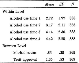
Table 7.1
Descriptive Statistics for Within- and Between-Level Variables
Between-Level Measures
Parents reported on their marital status, coded 0 = “Not married” or 1 = “Married.” Parents were also asked how wrong they felt it was for their children to use alcohol. This variable was labeled “tacit approval” and was coded 4 = “Not wrong at all,” 3 = “A little bit wrong,” 2 = “Wrong,” or 1 = “Very wrong.” These predictors were assessed at the first time point; thus, their effects are contemporaneous with initial status and precede growth. Descriptive statistics for the variables of interest are presented in Table 7.1.
STATISTICAL MODELING APPROACHES
This following section gives a brief overview of the modeling specifications for the three approaches used in this study: (a) a FIML LGM approach, (b) a limited information MLGM, and (c) HLM. Models were specified across the three approaches so that each would answer the same research question involving predictors of change in family-level alcohol use—and results from the different techniques could be directly compared.
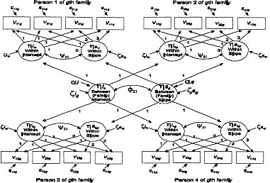
Figure 7.1: Factor-of-curves model (FIML LGM).
Full Information Maximum Likelihood
To test the degree to which relations among the growth factors for different family members could be described by a higher-order family construct, the latent growth curve model was parameterized as a factor-of-curves LGM (see Figure 7.1). This higher-order model follows a structure similar to a first-order multivariate associative LGM (e.g., Duncan et al., 1996; Muthén, 1990), but the covariances among the first-order factors are hypothesized to be explained by the higher-order latent growth factors. To represent the system of relationships in the model shown in Figure 7.1, three sets of equations are needed: (a) an equation modeling level 1 within-person data, (b) an equation modeling level 2 between-person within-family data, and (c) an equation modeling level 3 between-families data. Elaboration of these equations is presented subsequently.
The equation for modeling level 1 within-person data can be expressed as
where υjg is a vector of repeated measures representing the empirical growth record for individual j in the family g, Λυ is a fixed basis matrix containing a column of ones and a column of constant time values, η is a vector containing latent growth factors; ηjg′ = (ηijg, ηsjg), where ηiig represents initial status and ηsjg represents rate of change over time, and єjg is a vector containing measurement errors, where it is assumed that, for simplicity, Cov(єjg) is a diagonal matrix. Under this equation, the repeated measures data are represented as
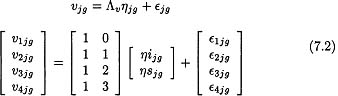
where in the Λυ matrix, column 1 defines initial status by fixing all factor loadings at 1 and column 2 defines the rate of change. Because previous findings have demonstrated relatively linear growth in alcohol use during adolescence (e.g., Duncan & Duncan, 1996), a basic growth model hypothesizing linear growth in alcohol use was tested by fixing the elements for the slope factor to known values (i.e., λ12 = 0, λ22 = 1, λ32 = 2, λ42 = 3), respectively, for each person. Setting λ12 = 0 on the slope factor allows interpretation of the latent growth factors, ηijg and ηsjg, as initial status at t = 0 and rate of change across time. The model can also accommodate nonlinear growth. For example, an unspecified model (i.e., freeing λ32 and λ42 parameters) enables the developmental trajectory for each person to be freely estimated, allowing for possible nonlinearity and maximal fit to the data (e.g., Duncan et al., 1997 and Meredith & Tisak, 1990).
The level 2 between-person equation considers individual variation within family as a function of family-level variation. As such, the model equation at this level can be expressed as
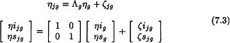
In this equation, ηjg is defined as before, the Λg is an identity matrix of within-family factor basis terms, ηg contains the gth family mean growth parameters ηig and ηsg. For model identification purposes, the latent means for the gth family contained in ηg are fixed to zero (a null vector). These means are estimated at level 3. ζjg is a vector containing disturbance terms (or residuals) associated with the regression of each of the lower-order factors, ηijg and ηsjg, with the variance-covariance matrix, Ψ, of latent residual parameters of the following form:
![]()
where the element of ψ21 in Ψ represents the covariance between the latent residual factors.
The level 2 equation model just described is further accounted for by the level 3 higher-order latent growth factors, which have the following form:
![]()
where α is a vector containing the latent growth means of the between-family latent growth parameters (i.e., α′ = (αi, αs) and ζg is a vector of deviation scores reflecting the family level variation (i.e., ζg′ = ηig – αi, ηsg – αs). Specifically, this model has the following latent growth vector form:
where αi and αs denote overall family mean values in initial status and rate of change and ζig and ζsg represent deviations of individual families growth parameters from the overall family means as defined earlier. The ζg vector is of special interest in this multilevel analysis because it represents family level variation. ζg is distributed with zero mean vector and covariance matrix Φ with the following parameter matrix:
where the element of ϕ21 in Φ denotes the covariation, at the family level, between initial status and rate of change over time.
To summarize, in Equations 7.1 through 7.7, the growth modeling provides for level 1 (within-individual; e.g., repeated observations), level 2 (between individual within family), and level 3 (between families) models that represent hypotheses about the growth structure underlying the repeated measures family data.
An extension of this model involves incorporating exogenous predictors of the growth factors at level 3, where such predictors may be measured or latent. For example, to incorporate exogenous predictors x, the model is written as
![]()
where x is the vector of exogenous predictors, ![]() x contains the mean vector, Λx is an identity matrix, ξ contains the exogenous predictors deviated from their means, and δ is a null vector. Centering the predictors of change ensures that the α vector in the growth portion of the model will retain its interpretation as the family mean vector of initial status and growth (see Willett & Sayer, 1994).
x contains the mean vector, Λx is an identity matrix, ξ contains the exogenous predictors deviated from their means, and δ is a null vector. Centering the predictors of change ensures that the α vector in the growth portion of the model will retain its interpretation as the family mean vector of initial status and growth (see Willett & Sayer, 1994).
In the present example, the family clusters are of varying size (i.e., unbalanced). Therefore, the analysis can be viewed as a regular multiple-group LGM with data missing for some families. Although unbalanced data can be accommodated in SEM analyses by expanding the usual structural equation model to include means, or regression intercepts, and partitioning the sample into subgroups with distinct data patterns (Duncan, Duncan, Strycker, Li, & Alpert, 1999), a FIML procedure, as implemented in many SEM software packages such as Mplus (Muthén & Muthén, 1998), Amos (Arbuckle, 1995), and Mx (Neale, 1991), represents a much simpler and more direct approach to handling unbalanced continuous data.
The current example contains only one form of missingness (i.e., unbalanced data), but the raw ML approach used for the factor-of-curves model also allows for data that can be considered missing by omission or missing by attrition, as long as the missing data mechanism can be considered ignorable. Thus, unlike any of the other multilevel methods presented here, the raw ML approach allows for unbalanced and/or missing data at each level of the hierarchy without the need for prior or two-stage multiple imputation procedures (see Duncan et al., 1999).
Limited Information Multilevel Latent Growth Modeling Analysis
The multilevel LGM approach of Muthén (1997) involves two generalizations of the factor-of-curves SEM model: (a) SEM growth modeling as generalized to cluster data and (b) SEM multilevel modeling as generalized to mean structures. Within the latent variable modeling of longitudinal and multilevel data, the total covariance matrix, ST, is decomposed into two independent components, a between-families covariance matrix, SB, and a within-families covariance matrix, SPW, or ST = SB + SPW. The multilevel latent growth model (MLGM) makes use of SPW and SB simultaneously.
Latent Growth Formulation
Muthén (1997) presented a latent variable formulation that can be applied to the three-level data case shown earlier. To express this hierarchical model in latent variable notation similar to that of Equation 7.1, we have
![]()
where υig is a 4 × 1 vector of observed outcomes for the four time points, Λυ a 4 × 2 matrix of factor loadings, ηjg a 2 × 1 vector of latent variables representing the growth parameters, and єig a 4 × 1 vector of error terms.
Figure 7.2 shows a path diagram for describing the model specification of Muthén’s (1997) latent variable growth model formulation for two-level, T = 4 data on the observed variables v. Again, assuming linear growth, there are two latent growth factors, ηi and ηs, representing initial status and rate of growth, respectively. Following structural modeling conventions, squares in Figure 7.2 denote observed variables and circles denote latent variables. The top part of the model refers to the between structure; the part below refers to the within structure.
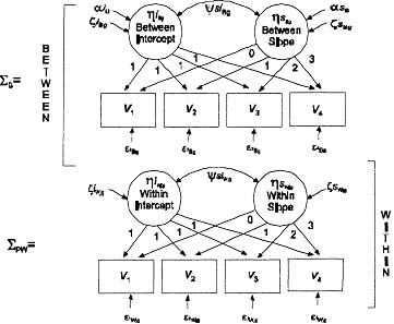
Figure 7.2: Multilevel latent growth model (MUML MLGM).
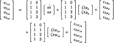
The MLGM model with between and within level decomposition can be written in matrix notation as
where the υig represents the repeated measures vector for the jth person (person; j = 1, 2, …, J) in the gth family (g = 1, 2, …, G). The first term on the right side of the equation represents the mean of the initial status and the mean of the linear growth rate. The second and third terms correspond to between-family variation. The fourth and fifth terms correspond to within-family variation. Writing out Equation 7.10, υjg yields the following matrix representation:
![]()
On the between-level component, we note that ζiBg and ζsBg factors correspond to the ζig and ζsg residuals of Equation 7.6, whereas the within-level ζiWjg and ζsWjg factors correspond to ζjg residuals of Equation 7.3 with the parameters of ζijg and ζsjg. The basis function matrix, Λ, for the between and within slope factors, is specified in a similar fashion as those described in the FIML factor-of-curves method. The influence from the two latent factors (ηi and ηs) is the same on the between component as it is on the within component. Corresponding to this specification, in Figure 7.2, the SB growth factor structure is identical to that of the SPW growth factor structure. This specification can, however, be altered by relaxing the constraints between the SB and SPW factor structures.
Both between- and within-level predictor variables (either observed or latent) can be incorporated into the model in Equation 7.10 to account for variation in person and family levels. For example, observed between-level variables xg (where x is a vector of exogenous family-level predictors) may be included to predict variation in the latent between-level variables. Similarly, observed within-level variables xjg can be incorporated into the model to explain variation at the person level.
Model Estimation
As can be seen from Figure 7.2, the MLGM approach significantly simplifies model specification. Rather than specifying separate LGMs for each family member, a single LGM represents growth for each person within the family. For actual estimation using the Mplus SEM program (Muthén & Muthén, 1998), a model must be specified for each level of data. Mplus is able to estimate models with two levels of data. However, for longitudinal designs, the repeated measures part of the model is not considered to be one of the two levels. Rather, it is treated as a multivariate measurement model in the form of a factor-analytic, multiple-indicator model for the repeated measures. Therefore, the model is set up with SB used as input for the between part of the model and SPW used as input for the within part of the model.
The two sample covariance matrices SPW, and SB are expressed as
![]()
and
![]()
Muthén (1994) demonstrated that the pooled within matrix, SPW, is a consistent and unbiased estimator of ∑W, while the between matrix, SB, is a consistent and unbiased estimator of ∑W + C ∑B, where C reflects the family size, computed as:
![]()
For unbalanced data, C is close to the mean of the family sizes. Note that the between-family matrix, SB, is the covariance matrix of family means weighted by the family size. Therefore, the ML estimate of ∑W is SPW, whereas the ML estimate of ∑B is
![]()
The fitting function that is minimized is
The top line of Equation 7.16 corresponds to the between part of the model setup, which captures the between-level contribution to the total variation, weighted by G, the number of families. The bottom line of the equation corresponds to the within part of the model, which captures the within-level contribution to the total variation, and is weighted by N - G, the total sample size minus the number of families. Note that for balanced data, C is the common family size and the two-group approach above is equivalent to FIML estimation. The mean structure for the MLGM arises from the four observed variable means for alcohol use, expressed as functions of the latent factor means of the ηi and ηs between-level factors. The means of the within-level growth factors are fixed at zero. For a complete exposition and computational details concerning ad hoc estimation procedures, see Muthén (1994). The FIML and MUML LGM analyses in the present study were performed using the Mplus SEM computer program (Muthén & Muthén, 1998).
A three-level HLM model was used for this example to account for longitudinal and family relations. The three-level model consists of three sub-models, one for each level. When defining the HLM model of interest, the level 1 equations model the observed person data for each time point. The level 2 equations model the individual level. The level 3 equations model the family level. Adopting notation from Bryk and Raudenbush (1992), a three-level, unconditional growth model (no predictors) for estimating change in alcohol use is described.
For the level 1 model, the equation is
where υtjg = the observed score at time t for person j in family g, π0jg = initial status for person jg, π1jg = growth rate for person jg, at = specified basis term (e.g., set a′ = [0 1 2 3] to correspond to the interpretation of the measurement occasion for person j in family g at time t = 0 as the initial status), and єtjg = within person random error, assumed to be independent and normally distributed with mean = 0 and constant variance σ2. Thus, change in alcohol use for each person j consists of two growth parameters: π0jg = initial status defined at t = 0, and π1jg = rate of change across the four measurement occasions. It should be noted that in HLM the basis terms must be specified by the user. This is different from both the FIML factor-of-curves and MLGM models, in which unspecified growth functions (i.e., basis parameters freely estimated by the software program) can be estimated.
The person-specific change parameters in Equation 7.17 become outcomes in the level 2 model for variation between persons. The simplest level 2 model enables us to estimate the mean trajectory and the extent of variation around the mean, which has the following equations:
and
![]() 1jg = β10g + r1jg
1jg = β10g + r1jg
where β00g = mean initial status within family g at t = 0, β10g = mean rate of change within family g across time, r denotes the person-specific random effect, with r0jg = deviation of person j’s initial status within family g at t = 0 from the mean of the gth family, and r1jg = deviation of person j’s rate of change within family g from the mean of the gth family growth rate. These random effects are assumed bivariate normally distributed with a 2 × 2 variance and covariance matrix, Tπ, of the following form:
![]()
where ![]() π00 is the variance in initial status at t = 0,
π00 is the variance in initial status at t = 0, ![]() π11 is the variance of the rate of change, and
π11 is the variance of the rate of change, and ![]() π10 is the covariance between status at t = 0 and rate of change.
π10 is the covariance between status at t = 0 and rate of change.
For the level 3 model, the growth parameters within family g become the outcomes of level 3 parameters, as expressed by the following equations:
and
β10g = γ100 + u10g
where γ000 = overall mean initial status, γ100 = overall mean growth rate, and u denotes random effect reflecting family variability, with u00g = family variation in status t = 0 and u10g = family variation in growth rate across time. The random effects at level 3 are assumed normally distributed with variance and covariance matrix:
![]()
where ![]() β00 is the variance in initial status at t = 0,
β00 is the variance in initial status at t = 0, ![]() β11 is the variance of the rate of change, and
β11 is the variance of the rate of change, and ![]() β10, is the covariance between status at t = 0 and rate of change.
β10, is the covariance between status at t = 0 and rate of change.
The specification of Equations 7.17, 7.18, and 7.20 can be further extended to incorporate predictors of variability associated with the levels 2 and 3—persons and families. Consider, for example, a single-time invariant predictor of initial status and growth for person j in the gth family denoted as xjg. Then, the level 2 model can be written as
![]()
and
π1jg = β10g + β11xjg + r1jg
One can also consider that xg, a level 3 predictor, is related to the family level variation (e.g., in our example xg represents marital status or tacit approval) giving rise to the following level 3 model
![]()
and
β10g = γ100 + γ101xg + u1g
The actual estimation procedure for the three-level model uses a full ML procedure to estimate both covariance components and the fixed effects (levels 2 and 3 coefficients). The HLM analyses in the present study were performed using the HLM program (Bryk, Raudenbush, & Congdon, 1996).
Full Information Maximum Likelihood
In accommodating analyses with unbalanced data, Mplus (Muthén & Muthén, 1998) treats the unbalance nature of the data as an incomplete or missing data problem and produces model parameter estimates using a ML fitting function. Fitting the basic factor-of-curves LGM produced the following chi-square fit statistic, χ2(143) = 372.776, p < .001, RMSEA = .066. Mplus program input for the unconditional factor-of-curves model is shown in Appendix A.2
Parameter estimates for the factor-of-curves model are shown in Table 7.2. Significant mean levels were evident for the common second-order intercept, αi, and common slope, αs, indicating growth in family levels of alcohol use over time. Between-level factor, ζig and ζsg, and within-level factor, ζijg and ζsjg, variances for the intercept and slope were also significant, indicating variation in the intercept and slope of alcohol use across families and individuals. The between- (family-level) to-total factor variance ratios for the intercept and slope suggest that approximately 31% and 42% of the individual variation in the intercepts and slopes, respectively, could be accounted for by family membership.
A factor-of-curves LGM with the inclusion of family-level predictors was also tested, resulting in the following chi-square fit statistic, χ2(171) = 414.945, p < .001, RMSEA = 0.62. Examination of the parameter estimates for this model indicated that the family-level predictor, parental tacit approval, was a significant predictor of the between-level intercept, β = .551, se = .142, t = 3.875. Greater tacit approval was associated with more pronounced levels of family alcohol use. The effects of marital status on the between-level intercept, β = –.085, se = .198, t = -.427, and the effects of marital status, β = . – 008, se = .071, t = -.116, and tacit approval, β = .041, se = .051, t = .806, on the between-level slope were not significant.
Table 7.2: Parameter Estimates for the Unconditional Growth Curve Models
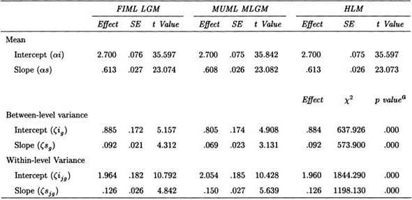
aHLM program provides chi-square test statistics for the random effects (i.e., variance components of the model).
Limited Information Multilevel Latent Growth Modeling Analysis
The MLGM model tested incorporated a two-factor latent growth structure for both within and between levels.3 Model-fitting procedures produced a chi-square test statistic of χ2(14) = 151.255, p < .001, RMSEA = .105. Mplus program input for the unconditional MLGM is presented in Appendix B. Parameter estimates for the factor-of-curves model are shown in Table 7.2. Significant mean levels were evident for the common second-order intercept, αi, and common slope, αs, indicating growth in family levels of alcohol use over time. Similar to those from the FIML analysis, between-level factor, ζig and ζsg, and within-level factor, ζijg and ζsjg, variances for the intercept and slope were also significant, indicating variation in the intercept and slope of alcohol use across families and individuals. The significant between-level variances indicated that substantial heterogeneity existed among typical families.
The between- (family-level) to-total factor variance ratios for the intercept and slope suggest that approximately 28% and 32% of the individual variation in the intercepts and slopes, respectively, could be accounted for by family membership.
In the MLGM with family-level predictors, the family-level variables can be seen as influencing the family-level part of the individual family members’ slopes and intercepts indirectly through the family-level factor components. Although the within part of the model is that of a regular two-factor LGM, the between part allows for correlations among the between components of the alcohol use variables that are explained not only by the two common factors but also by correlations via the predictors and their direct and indirect effects.
Fitting the two-factor structural latent growth model to the data resulted in a chi-square test statistic of χ2(18) = 163.168, p < .001, RMSEA = .095. The family-level predictor, parental tacit approval, was a significant predictor, β = .529, se = .141, t = 3.754, of the between-level intercept. The effects of marital status on the between-level intercept, β = –.084, se = .196, t = -.426, and the effects of marital status, β = –.012, se = .070, t = –.070, and tacit approval, β = .040, se = .050, t = .804, on the between-level slope were not significant.
Hierarchical Linear Modeling
Parameter estimates for the unconditional HLM three-level model using the HLM heierarchical linear modeling software program of (Bryk et al., 1996) are presented in Table 7.2. HLM program input for the unconditional model is presented in Appendix C. Significant mean levels were evident for the intercept and slope, indicating growth in family levels of alcohol use over time. Approximately 31% and 42% of the individual variation in the alcohol intercept and slope scores, respectively, is between families (level 3). The significant level 3 variance indicated that there was significant variability in the families’ intercepts and slope scores. These parameters can be treated as outcomes. With the inclusion of predictors at the third level, family deviations can be predicted from the grand mean. Parameter estimates for this intercept- and slope-as-outcomes HLM resulted in similar parameter estimates with parental tacit approval emerging as a significant predictor, β = .550, se = .141, t = 3.891, of the between-level intercept. The effects of marital status on the between-level intercept, β = –.087, se = .193, t = -.449, and the effects of marital status, β = –.008, se = .068, t = –.121, and tacit approval, β = .042, se = .050, t = .847, on the between-level slope were not significant.
DISCUSSION
The aim of the present study was to compare results across three different statistical approaches to modeling multilevel longitudinal alcohol use data. The research question involved development in family-level alcohol use over a 4-year period and the effects of family-level predictors of marital status and parental tacit approval on adolescent alcohol use.
From a substantive point of view, several results are worth noting. First is the significant upward trend in the development of alcohol use among families. This finding is consistent with other developmental studies (e.g., Duncan, Duncan, & Hops, 1996) that have assessed the developmental nature of alcohol use among adolescents. Moreover, significant variation in alcohol use and development existed across families. Given this variation in alcohol use, it was of interest to determine if the family variation in alcohol use scores could be accounted for by family-level covariates. Thus, contextual variables were used to explain the heterogeneity in alcohol use among families.
The most interesting finding of this study was the effect of parental tacit approval of alcohol use on the between-level intercept for alcohol use. Results of all analyses indicated that, the more parents viewed alcohol use as an acceptable behavior for their children, the greater the initial level of family alcohol use. This finding adds support to other studies that suggest “permissive” parental attitudes are an important influence on adolescent alcohol use behaviors (Barnes & Welte, 1986; Brook et al., 1986; McDermott, 1984). The effects of marital status on the between-level intercept, and the effects of marital status and tacit approval on the between-level slope, were not significant in any of the analyses.
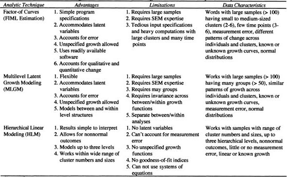
The similarity in results of the three approaches suggests that in many cases there may be no one “correct” way to analyze multilevel longitudinal data. All three of the analytic techniques were able to answer the research questions regarding homogeneity in alcohol use development among siblings and predictors of alcohol use across families. Models were specified to ensure that growth functions (e.g., linear growth) and, as a result, findings were similar across these techniques. Researchers should ultimately select an analytic technique based on the benefits and limitations of the approach as well as appropriateness to the research question. The following sections outline some of the advantages and limitations (summarized in Table 7.3) of each of the three analytic approaches presented in this chapter.
Full Information Maximum Likelihood Factor-of-Curves LGM
The FIML LGM approach presented was an extension of higher-order factor analytic methods. The factor-of-curves model used in the present study describes individual differences within separate univariate series and forms a common factor model to describe individual differences among these basic growth curves. In practice, this multivariate extension offers researchers opportunities for evaluating the dynamic structure of both intra- and interindividual change.
The higher-order LGM approach using FIML estimation has several attractions in the analysis of longitudinal multilevel data. It takes into account all available data and produces consistent and efficient estimates. The approach is also favored for its simplicity in program specification and flexibility in handling unbalanced data.
The ability to handle missing data at each level of the hierarchy is especially noteworthy. Although the current example incorporated only unbalanced data (i.e., data that might be considered missing by design), the FIML approach allows for data that can also be considered missing by omission (i.e., a subject fails to complete an item within a survey or fails to complete a survey) or missing by attrition (i.e., some participants drop out of the study and are not remeasured, a common problem for longitudinal studies) as long as the missing data mechanism can be considered ignorable (see Graham, Hofer, & Piccinin, 1994 for a complete discussion). The FIML approach takes into consideration all available causes of missingness and employs the same statistical model to handle the missing data that is used to perform the desired analysis. Standard errors are a convenient by-product of the analysis.
The factor-of-curves approach has other benefits. Conducted within the SEM framework, the factor-of-curves model can include latent variables and thus account for measurement error. This technique also can handle some types of nonlinear trajectories (unspecified growth functions) for each family member. Rather than focusing solely on quantitative change, using invariant growth functions across all family members, this approach has the potential to allow for modeling qualitative differences among family members. For example, Zajonc and Mullally (1997) introduce the concept of collective potentiation that specifies collective side effects of birth order. They argue that, in contrast to genetic theories that have repeatedly down-sized and outsourced environmental factors such as family influences, their confluence model quantifies the differential environmental contributions to development of successive siblings. The assumption is that the qualitative differences are quantifiable and that they would define an emerging second-order family growth factor (see Patterson, 1995, for an example of analyses of qualitative shifts in factor patterns over time). Finally, the FIML model can be estimated using a number of currently available SEM software programs.
Table 7.3: Advantages and Limitations of Three Longitudinal Multilevel Analytic Techniques
The FIML approach also has limitations. This technique requires large samples and some SEM expertise. With large group sizes, the input specifications can be tedious and estimation tenuous. In the present example, model specification included 4 repeated measures for each of a maximum of 4 family members, resulting in 16 observed dependent variables. With the inclusion of covariates, a total of 18 variables were modeled. As the number of time points and number of family members increase, the total number of variables to be modeled increases, as does model complexity. Increased complexity can decrease the likelihood of achieving an acceptable solution.
Although model-fitting procedures in the present study revealed similarities between the factor-of-curves and other multilevel approaches, this may not be the case with different data structures and assumptions concerning factorial invariance of the growth parameters across individuals. Because both empirical and substantive differences may be critical for correct interpretation of the dynamics and influences of change, further applications of these approaches investigating both qualitative and quantitative change should be pursued.
Limited Information Multilevel Latent Growth Modeling Analysis
The MLGM uses a two-stage approach to model estimation. In the first stage, the total variance-covariance matrix is decomposed into within, SPW, and between, SB, components. In the second stage, the MLGM model is specified using both SB and SPW matrices within the SEM framework. The developers of Mplus have made this two-stage approach inconspicuous for the user. In doing so, the MLGM, as operationalized within Mplus, greatly simplifies model specification. Rather that dealing with a model incorporating 16 observed variables (4 repeated measures on 4 family members) the model is specified using only the 4 repeated measure variables.
The flexibility of the basic MLGM approach makes it an attractive analytic tool for a variety of SEM analyses with longitudinal multilevel data. Like the full ML model, the limited information approach has the capacity to estimate and test relationships among latent variables and account for measurement error. It explicitly models the within- and between-level co-variance matrices while avoiding the problems of FIML when group sizes are large. Muthén (1994) shows that this simpler estimator is consistent, is identical to the FIML estimator for balanced data, and gives results close to those of FIML for data that are not too badly unbalanced.
Limitations of this technique include the necessity of SEM experience, large samples, and a sizable number of groups. Although MLGM allows for the specification of nonlinear trajectories, unlike the FIML approach it requires that these trajectories are invariant across all family members and requires that the contribution of the common between-level factor to the within-level growth functions be equal across individuals. At present, the MLGM approach is also unable to handle data that are missing by omission or attrition without separate imputation procedures being employed because of its limited information approach.
Hierarchical Linear Modeling
HLM efficiently examines questions about the hierarchical nature of longitudinal alcohol use data within the regression format. Its use of regression notation makes interpretation and dissemination of results relatively simple. At present, HLM can explicitly model up to three levels of data, which is an advantage few programs offer. Three kinds of parameter estimation are available in a three-level HLM model: empirical Bayes estimates of randomly varying level 1 and level 2 coefficients, ML estimates of the level 3 coefficients (there are also generalized least square estimates), and ML estimates of the variance-covariance components.
HLM can handle nonnormal outcomes and incorporates some forms of missing data. The HLM approach is able to handle missingness at level 1 only, through pairwise and listwise deletion of cases. These approaches follow the conventional routines used in standard GLM procedures found in most statistical packages. Clearly, with substantial missingness, these approaches should be used with caution given the likelihood of resulting nonpositive definite covariance matrices. Another plus is that HLM functions well within a wide range of cluster numbers and sizes.
Drawbacks of the HLM approach include its inability to readily allow for the specification of systems of structural equations at the within and between levels of clustering (i.e., variables cannot be specified as both independent and dependent in the same analysis; Kaplan & Elliott, 1997). Unlike both the FIML LGM and MLGM approaches, HLM is unable to fit unspecified growth functions (basis parameters freely estimated by the software program), although specific nonlinear functions can be designated with known values by the user. Qualitative differences among family members, therefore, cannot be accommodated using this method. Also, unlike the SEM-based approaches (i.e., FIML LGM and MLGM), HLM provides no overall goodness-of-fit indices, although HLM does allow the user to easily conduct residual analyses for checking model accuracy.
Three approaches for the analysis of clustered and/or longitudinal data that may contain multiple levels were compared in this chapter. These procedures are sometimes referred to as random effects (e.g., Stiratelli, Laird, & Ware, 1984), hierarchical, mixed effects, multilevel, or cluster-specific models. Results show that all three analytic procedures emerged as viable methods for use with multilevel, longitudinal data and that they represent different ways of modeling data with repeated observations.
Researchers should weigh the advantages and limitations of the different approaches in relation to their research questions when selecting a technique. Decisions will necessarily be influenced by aspects such as normality of the data, sample size, latent variable format needs, missing data, factorial variance/invariance, and the number of levels to be modeled as well as accessibility, ease, and experience. The flexibility of these techniques make them attractive analytic tools for a variety of analyses investigating growth and development among variables of interest with multilevel data. Within the specific area of adolescent behavior, hierarchical models allow for potentially greater insight into the developmental nature, antecedents, and sequelae of a variety of adolescent problem behaviors.
APPENDIX A
TITLE:
Multivariate growth model for alcohol use observed over four time points for each family member. Families of size 2, 3, and 4. Linear growth. Same growth model functions for each family member. Missing data analysis.
Growth process: v1, v2, v3, v4 - family member 1
v5, v6, v7, v8 - family member 2
v9, v10, v11, v12 - family member 3
v13, v14, v15, v16 - family member 4
DATA:
FILE IS focms.dat;
VARIABLE:
NAMES ARE vl_v16;
MISSING = ALL (99.00);
USEVAR = vl_v16;
ANALYSIS:
TYPE = MEANSTRUCTURE MISSING H1;
COVERAGE=.05;
MODEL:
wint1 BY vl_v4@1;
wslp1 BY v1@0 v2@1 v3@2 v4@3;
wint2 BY v5_v8@1;
wslp2 BY v5@0 v6@1 v7@2 v8@3;
wslp3 BY v9@0 v10@1 v11@2 v12@3;
wint4 BY v13_v16@1;
wslp BY v13@0 v14@1 v15@2 v16@3;
[vi_v16@0];
bint by wint1@1 wint2@1 wint3@1 wint4@1;
bslp by wslp1@1 wslp2@1 wslp3@1 wslp4@1;
[bint bslp];
[wint1@0 wint2@0 wint3@0 wint4@0];
[wslp1@0 wslp2@0 wslp3@0 wslp4@0];
bint WITH bslp;
vl-v16(1);
wslp1 wslp2 wslp3 wslp4 PWITH wint1 wint2 wint3 wint4(5);
wint1_wint4(6);
wslp1_wslp4(7);
OUTPUT: STANDARDIZED;
APPENDIX B
TITLE:
Growth model for alcohol use observed over four time points. Linear growth. Complex sample analysis, multilevel modeling (disaggregated modeling). Same growth model functions for between_and within_level model parts.
Growth process: v1, v2, v3, v4
DATA:
FILE IS ms.dat;
FORMAT is 9f8.2;
VARIABLE:
NAMES ARE g1 g2 vl v2 v3 v4 xl x2 cluster;
USEVAR = vl_v4;
CLUSTER = cluster;
ANALYSIS: TYPE = TWOLEVEL;
ITERATIONS = 100;
ESTIMATOR = ML;
MODEL:
%BETWEEN%
bint BY v1_v4@1;
bslp BY v1@0 v2@1 v3@2 v4@3;
[v1_v4@0];
[bint_bslp];
bint WITH bslp;
v1(1);
v2(1);
v3(1);
v1(2);
v2(2);
v3(2);
v4(2);
%WITHIN%
wint BY v1_v4@1;
wslp BY v1@0 v2@1 v3@2 v4@0;
wint WITH wslp;
v1(2);
v2(2);
v3(2);
v4(2);
OUTPUT: SAMPSTAT STANDARDIZED;
| HLM Setup | Comment |
| Levell: ALC=INTRCPT1+LIN | Level 1 model (see Equation 7.17) |
| Level2: INTRCPTl=INTRCPT2+random/ | Level 2 model for π0jg in Equation 7.18 |
| Level2: LIN=INTRCPT2+random/ | Level 2 model for π1jg in Equation 7.18 |
| Level3: INTRCPT2=INTRCPT3+random/ | Level 3 model for β00g in Equation 7.20 |
| Level3: INTRCPT2=INTRCPT3+random/ | Level 3 model for β10g in Equation 7.20 |
| Nonlin: N | A nonlinear analysis is not requested |
| Numit: 100 | Request for maximum of 100 iterations |
| Stopval: 0.000001 | 0.000001 is the convergence criterion |
| Fixtau2: 3 | Option 3, “automatic fixup”, invoked if variance-covariance matrix at Level 2 is not positive definite |
| Fixtau3: 3 | Option 3, “automatic fixup”, invoked if variance-covariance matrix at Level 3 is not positive definite |
| Accel: 5 | Controls interaction acceleration. Default is 5 |
| Resfil2: N | No Level 2 residual file will be output |
| Resfil3: N | No Level 3 residual file will be output |
| Hypoth: N | No optional hypothesis testing requested |
| CONSTRAIN: N | No equality constraints imposed on fixed effects |
| Title: Growth curve modeling using HLM | Title of the setup |
| Output: HLM.out | Results be saved in HLM.out |
Preparation of this manuscript was supported by Grant DA11942 and Grant DA09548 from the National Institute on Drug Abuse and Grant AA11510 from the National Institute on Alcohol and Alcoholism. The National Youth Survey was supported by Grant MH27552 from the National Institute of Mental Health.
REFERENCES
Aitkin, M., & Longford, N. (1986). Statistical modeling issues in school effectiveness studies. Journal of the Royal Statistical Society, 149, 1–43.
Akers, R. L., & Cochran, J. E. (1985). Adolescent marijuana use: A test of three theories of deviant behavior. Deviant Behavior, 6, 323–346.
Arbuckle, J. L. (1995). Amos user’s guide. Chicago, IL.
Bandura, A., & Walters, R. H. (1963). Social learning and personality development. New York: Holt, Rinehart and Winston.
Barnes, G. M., & Welte, J. W. (1986). Patterns and predictors of alcohol use among 7–12th grade students in New York state. Journal of Studies on Alcohol, 47, 53–62.
Brook, J. S., Gordon, A. S., Whiteman, M., & Cohen, P. (1986). Some models and mechanisms for explaining the impact of maternal and adolescent characteristics on adolescent stage of drug use. Developmental Psychology, 22, 460–467.
Bryk, A. S., & Raudenbush, S. W. (1992). Hierarchical linear models: Applications and data analysis methods. Newbury Park, CA: Sage.
Bryk, A. S., Raudenbush, S. W., & Congdon, R. T. (1996). HLM: Hierarchical linear and nonlinear modeling with the HLM/2L and HLM/3L programs. Chicago, IL: Scientific Software International, Inc.
Burstein, L. (1980). The analysis of multilevel data in educational research and evaluation. Review of Research in Education, 8, 158–233.
Byram, O. W., & Fly, J. W. (1984). Family structure, race, and adolescents’ alcohol use: A research note. American Journal of Drug and Alcohol Abuse, 10, 467–478.
Capaldi, D. M. (1989). The relation of family transitions and disruptions to boys’ adjustment problems. (Paper presented at the conference of the Society for Research in Child Development, Kansas City, MO)
Capaldi, D. M., & Patterson, G. R. (1991). Relation of parental transitions to boys’ adjustment problems: I. A linear hypothesis. II. Mothers at risk for transitions and unskilled parenting. Developmental Psychology, 27, 489–504.
de Leeuw, J., & Kreft, I. (1986). Random coefficient models for multilevel analysis. Journal of Educational Statistics, 11, 57–85.
Duncan, S. C., & Duncan, T. E. (1996). A multivariate latent growth curve analysis of adolescent substance use. Structural Equation Modeling, 3, 323–347.
Duncan, S. C., Duncan, T. E., & Hops, H. (1996). Analysis of longitudinal data within accelerated longitudinal designs. Psychological Methods, 1, 236–248.
Duncan, T. E., Duncan, S. C., Alpert, A., Hops, H., Stoolmiller, M., & Muthén, B. (1997). Latent variable modeling of longitudinal and multilevel substance use data. Multivariate Behavioral Research, 32, 275–318.
Duncan, T. E., Duncan, S. C., & Hops, H. (1998). Latent variable modeling of longitudinal and multilevel alcohol use data. Journal of Studies on Alcohol, 59, 399–408.
Duncan, T. E., Duncan, S. C., Hops, H., & Stoolmiller, M. (1995). An analysis of the relationship between parent and adolescent marijuana use via generalized estimating equation methodology. Multivariate Behavioral Research, 30, 317–339.
Duncan, T. E., Duncan, S. C., Strycker, L. A., Li, F., & Alpert, A. (1999). An introduction to latent variable growth curve modeling: Concepts, issues, and applications. Mahwah, NJ: Lawrence Erlbaum Associates.
Elliott, D. (1976). National Youth Survey [United States]: Wave I [Computer file]. ICPSR version. Boulder, CO: University of Colorado, Behavioral Research Institute [producer], (1977). Ann Arbor, MI: Inter-University Consortium for Political and Social Research [distributor], (1994).
Farrington, D. P. (1987). Early precursors of frequent offending. In J. Q. Wilson & G. C. Loury (Eds.), From children to citizens: Families, schools, and delinquency prevention (Vol. III, p. 27–51). New York: Springer-Verlag.
Flewelling, R. L., & Bauman, K. E. (1990). Family structure as a predictor of initial substance use and sexual intercourse in early adolescence. Journal of Marriage and the Family, 52, 1106–1111.
Goldstein, H. I. (1986). Multilevel mixed linear model analysis using iterative general least squares. Biometrika, 73, 43–56.
Graham, J. W., Hofer, S. M., & Piccinin, A. M. (1994). Analysis with missing data in drug prevention research. In L. M. Collins & L. Seitz (Eds.), Advances in data analysis for prevention intervention research. National Institute on Drug Abuse Research Monograph Series (#142). Washington, DC: National Institute on Drug Abuse.
Kandel, D. B., & Andrews, K. (1987). Processes of adolescent socialization by parents and peers. The International Journal of the Addictions, 22, 319–342.
Kaplan, D., & Elliott, P. R. (1997). A didactic example of multilevel structural equation modeling applicable to the study of organizations. Structural Equation Modeling, 4, 1–24.
Kreft, I. G. (1992). Multilevel models for hierarchically nested data: Potential applications in substance abuse prevention research. In L. Collins & L. Seitz (Eds.), Technical review panel on advances in data analysis for prevention intervention research. NIDA Research Monograph, 108.
Longford, N. T. (1987). A fast scoring algorithm for maximum likelihood estimation in unbalanced mixed models with nested effects. Biometrika, 74, 817–827.
Mason, W. M., Wong, G., & Entwistle, B. (1984). Contextual analysis through the multilevel linear model. In S. Leinhardt (Ed.), Sociological methodology (p. 72–103). San Francisco, CA: Jossey-Bass.
McArdle, J. J. (1988). Dynamic but structural equation modeling of repeated measures data. In J. R. Nesselroade & R. B. Cattell (Eds.), Handbook of multivariate experimental psychology (2nd ed.). New York: Plenum Press.
McDermott, D. (1984). The relationship of parental drug use and parent’s attitude concerning adolescent drug use to adolescent drug use. Adolescence, 19, 89–97.
Meredith, W., & Tisak, J. (1990). Latent curve analysis. Psychometrika, 55, 107–122.
Muthén, B. (1994). Multilevel covariance structure analysis. Sociological Methods & Research, 22, 376–398.
Muthén, B. (1997). Latent variable modeling of longitudinal and multilevel data. In A. Raftery (Ed.), Sociological methodology (p. 453–480). Boston, MA: Blackwell.
Muthén, B., & Satorra, A. (1989). Multilevel aspects of varying parameters in structural models. In R. D. Bock (Ed.), Multilevel analysis of educational data (p. 87–99). San Diego, CA: Academic Press.
Muthén, B. O. (1990). Mean and covariance structure analysis of hierarchical data. (Paper presented at the Psychometric Society meeting, Princeton, NJ)
Muthén, B. O. (1991). Analysis of longitudinal data using latent variable models with varying parameters. In L. C. Collins & J. L. Horn (Eds.), Best methods for the analysis of change (p. 1–17). Washington, DC: American Psychological Association.
Muthén, L. K., & Muthén, B. O. (1998). Mplus user’s guide. Los Angeles: Muthéen and Muthén.
Neale, M. C. (1991). Mx: Statistical modeling (Tech. Rep.). Box 3 MCV, Richmond, VA: Department of Human Genetics.
Patterson, G. R. (1995). Orderly change in a stable world: The antisocial trait as a chimera. In J. M. Gottman (Ed.), The analysis of change (p. 83–101). Mahwah, NJ: Lawrence Erlbaum Associates.
Raudenbush, S. W., & Bryk, A. S. (1988). Methodological advances in studying effects of schools and classrooms on student learning. In E. Z. Roth (Ed.), Review of research in education (p. 423–475). Washington, DC: American Educational Research Association.
Searle, S. R., Casella, G., & McCulloch, C. E. (1992). Variance components. New York: Wiley.
Stiratelli, R., Laird, N., & Ware, J. H. (1984). Random-effects models for serial observations with binary response. Biometrics, 40, 961–971.
Sweetser, D. A. (1985). Broken homes: Stable risk, changing reasons, changing forms. Journal of Marriage and the Family, 47, 709–715.
Thompson, K., & Wilsnack, R. (1984). Drinking problems among female adolescents: Patterns and influences. In S. Wilsnack & L. Beckman (Eds.), Alcohol problems in women (p. 37–65). New York: Guilford.
Willett, J. B., & Sayer, A. G. (1994). Using covariance structure analysis to detect correlates and predictors of individual change over time. Psychological Bulletin, 116, 363–381.
Winer, B. J. (1971). Statistical principles in experimental design (2nd ed.). New York: McGraw-Hill.
Zajonc, R. B., & Mullally, P. R. (1997). Birth order: Reconciling conflicting effects. American Psychologist, 52, 685–699.
__________________________________
1Elliot, D. National Youth Survey [United States]: Wave 1, (1976) [Computer file]. ICPSR version. Boulder, CO: University of Colorado, Behavioral Research Institute [producer], (1977). Ann Arbor, MI: Inter-University Consortium for Political and Social Research [distributor] (1994).
2In estimating the factor-of-curves model, the same growth function is fit to the repeated measures for each member of a particular family (e.g., linear growth) and the contribution of the family-level factors are the same for each family member. To provide comparable results to the other methods, and given the restrictions of fixed basis terms and regression parameters relating the first- and second-order factors, four within-level parameters, specified to be equal across family members (the latent within-level disturbances, ζiig and ζsig, within-level errors, єtjg, and within-level covariances, ψ21, and 5 between-level parameters (ζig, ζsg, φ21, αi, and αs), were estimated in the test of the hypothesized factor-of-curves model.
3In the specific growth model shown in Figure 7.2, the mean structure arises from the four observed variable means being expressed as functions of the means parameters αi and αs, here applied on the between side as shown in Equation 7.10. In the model estimation, the means are included in the between-level with a scaling constant (of family size) whereas the means on the within component are fixed at zero. This implies that dummy zero means are entered for the within family component.