
Dynamic Factor Analysis Models for Representing Process in Multivariate Time-Series
The University of Virginia
Virginia Commonwealth University
The University of Virginia
The collection of multivariate time-series and their analysis with mathematical models is necessary if we are effectively and fully to represent process and change. Among the promising applications currently available are variations of the common factor model that integrate factor and time series modeling features in a common analytic framework. We highlight some differences and similarities between two kinds of time series models for common factors: a direct autoregressive factor score (DAFS) model and a white-noise factor score (WNFS) model. Particular specifications of these models are fitted to data reflecting short-term changes in an intensively measured individual’s self-reported affect. Results of the model fitting underscore the importance of explicit differences in model specifications that define one’s view of the nature of process and change.
In various guises, the common factor model has been applied to multivariate time-series data for more than 50 years in effort to represent process and other kinds of change (Cattell, Cattell, & Rhymer, 1947; Hershberger, Molenaaar, & Corneal, 1996; McArdle, 1982; Molenaar, 1985; Wood & Brown, 1994). Despite the fact that particular applications of the model have been controversial (Anderson, 1963; Cattell, 1963b; Holtzman, 1963; Molenaar, 1985; Steyer, Ferring, & Schmitt, 1992), the logic underlying its use seems to be sound (e.g., Bereiter, 1963), and the results have been instrumental in the development of important lines of behavioral research such as the trait-state distinction (Cattell, 1957, 1961; Horn, 1972; Kenny & Zautra, 1995; Nesselroade & Ford, 1985; Singer & Singer, 1972; Steyer et al., 1992). These applications have helped to fuel a long-standing interest in intraindividual variability as a source of measurable individual differences (Baltes, Reese, & Nesselroade, 1977; Cattell, 1957; Eizenman, Nesselroade, Featherman, & Rowe, 1997; Fiske & Maddi, 1961; Fiske & Rice, 1955; Flugel, 1928; Kim, Nesselroade, & Featherman, 1996; Larsen, 1987; Magnusson, 1997; Nesselroade & Boker, 1994; Valsiner, 1984; Wessman & Ricks, 1966; Woodrow, 1932, 1945; Zevon & Tellegen, 1982). In this chapter, we briefly examine some of the history and key issues of factor analyzing multivariate time-series and, to exemplify the methods, present analyses of some promising recent developments aimed at further improving such applications.
In the broader context of applying covariation designs to the study of behavioral phenomena, the application of the common factor model to the data obtained when one individual is measured many times on many variables—multivariate time-series—has been called P-technique factor analysis (Cattell, 1952, 1961; Jones & Nesselroade, 1990; Luborsky & Mintz, 1972; Nesselroade & Ford, 1985). The analytical focus is on building a structural representation of patterns of within-person fluctuation of the variables over time. The intention of Cattell et al. (1947) in introducing this method of analysis was to discover “source traits” at the individual level. Cattell (1966) argued for some congruence between the way people change and the way they differ from each other. He declared that “we should be very surprised if the growth pattern in a trait bore no relation to its absolute pattern, as an individual differences structure” (p. 358) thus arguing for a similarity of patterns of intraindividual change and interindividual differences (Hundleby, Pawlik, & Cattell, 1965). Bereiter (1963) noted that correlations between measures over individuals should bear some correspondence to “correlations between measures for the same or randomly equivalent individuals over varying occasions, and the study of individual differences may be justifiable as an expedient substitute for the more difficult P-technique.” (p. 15) The flip side of this interpretation, which is not so often played, is that some of what are interpreted to be individual differences structures are actually intraindividual variability patterns that are asynchronous across persons and (perhaps erroneously) frozen in time by limiting the observations to a single measurement occasion. A key concern in either case is the degree of convergence between patterns of within-person change and among-person differences. Other authors have discussed this general topic under the label ergodicity (e.g., Jones, 1991; Nesselroade & Molenaar, 1999). The essential point is that investigation of variation (and covariation) in the individual over time is a meaningful and necessary enterprise, the results of which need to be integrated into the larger framework of behavioral research and theory.
Since 1947 a large number of P-technique studies have been conducted (see Luborsky & Mintz, 1972; Jones & Nesselroade, 1990, for reviews). By the early 1960s, neither the proponents of P-technique factor analysis such as Cattell nor its critics such as Holtzman (1963) were satisfied with its ability to model the subtleties of intraindividual change. Consider, for example, the matter of influence exerted on observed variables by the unobserved factors. The common factor model as traditionally applied to individual differences information (e.g., ability test scores) implies that individual differences in the underlying factors are responsible for individual differences in the observed variables. In P-technique applications, however, there are no individual differences because only one person is measured. Rather, the differences are in that individual’s scores from one occasion to another, that is, they are changes. Changes in the underlying factors are modeled as producing changes in the observed variables.
The original P-technique model implies that the total influence of a factor on an observed variable is exerted instantaneously. Restricting the coupling between factors and variables in this way implies that, on those occasions when the factor score is extreme, the variable score will also tend toward the extreme and, on those occasions when the factor score is moderate, the variable score will also tend to be moderate. The model does not afford explicit representation of more intricate (read realistic) patterns of influence of factors on variables such as persistence over time (e.g., the gradual dissipation or strengthening of the effects of extreme factor scores on one occasion on the variables at a later occasion). Moreover, the pattern of effect gradients may differ with different observed variables. Statements of the type “I’m okay now, I just can’t seem to stop shaking” illustrate the differences in the rates at which various components of a response pattern (e.g., self-reported internal state and objectively verifiable physical manifestations) return to equilibrium after the organism experiences an extreme in level of anxiety or fear. The basic P-technique model simply does not have the ability to represent the rich variety of relationships that we tend to associate with notions of process.
Cattell (1963b) himself called for refinements in the P-technique model that would allow representation of the effects exerted on the variables by the factors to dissipate or strengthen gradually over time rather than to be merely concurrent. It was not until the 1980s, however, that some key attempts to elaborate the P-technique factor model appeared that improved its capacity to represent change processes more veridically (e.g., Engle & Watson, 1981; Geweke & Singleton, 1981; McArdle, 1982; Molenaar, 1985). It is only in the past decade that the implementation of more promising, rigorous approaches to the study of intensively measured intraindividual variability in the single case via multivariate modeling has begun seemingly in earnest. In the remainder of this chapter we focus on two of these approaches, labeled the DAFS (direct autoregressive factor score) and WNFS (white noise factor score) models. We provide descriptions of the models and an example of fitting them to data. In so doing, we draw further attention to the evolving interest in intraindividual variability phenomena in a wide variety of content domains and identify some research tools that seem particularly promising for rapid advance in these areas. To illustrate the applications concretely, the factor models will be presented, discussed, and compared in the context of fitting them to real data using standard structural equation modeling software (e.g., LISREL 8 by Jöreskog & Sörbom, 1993).
LINEAR STRUCTURAL EQUATION MODELS FOR TIME-SERIES
We begin the presention of these linear structural equation models for multivariate time-series with a brief review and critique of the basic P-technique factor analysis model. The alternative specifications are then presented, fitted to empirical data, the results are described and discussed, and some implications for future research are drawn.
Basic P-Technique Factor Analysis Model
The essential novelty of the initial application of the common factor model to P-technique data (Cattell et al., 1947) was the fitting of the factor model to the covariation of multiple variables measured across time on only one individual. The P-technique application of the common factor model contrasts sharply with the usual one of fitting the model to the pattern of covariation of multiple variables measured across a sample of persons on a single occasion (R-technique factor analysis). Although in both cases one analyzes a symmetric, “variables × variables” covariance matrix, in P-technique the elements signify the extent to which the variables covary with each other over time (within one individual) whereas in R-technique the covariance elements indicate the extent to which the variables covary across persons (based on a single occasion of measurement).
For the traditional P-technique application, no accommodations are made in the basic factor model for time-related dependencies in the data. The traditional common factor model is applied straightforwardly to the multivariate time-series data. This factor model can be represented as
![]()
where y(t) is a p-variate observed time-series measured at time t(t = 1, 2, …, T), Λ is a p × k matrix of factor loadings, f (t) is a k-variate time-series of (unobserved) factor scores at time t (t = 1, 2, …, T), and u(t) is a p-variate time-series of unique parts (specificity plus error) of the observed scores at time t (t = 1, 2, …, T) that may have an autocorrelational but no cross-correlational structure. In fitting the common factor model to observed multivariate time-series, time-dependent properties of the common factor scores are ignored and the unique parts of the observed scores are assumed to be “white noise.” A path diagram of the model is represented in Figure 9.1.
As the time index t indicates, the factors are modeled as exerting their influence on the variables, but only concurrently in relation to the successive occasions of measurement. Thus, on a given occasion, a given observed score is constituted as a linear combination of the factor score(s) at that occasion of measurement and the “unique part” of that variable at that occasion. No lagged effects (e.g., the influence of yesterday’s factor score on today’s observed variable score) are represented in this model. Thus, the model’s ability to represent explicitly aspects of process is limited to concurrent relationships. Similarly, no time-dependent structure is recognized for the unique parts of the variables. In a covariance or correlation metric, the expectation for a unique part on a given day is zero, regardless of the magnitude of the unique part on the previous occasion.
As was noted earlier, this initial P-technique factor model was criticized by a number of writers (Holtzman, 1963; Molenaar, 1985; Steyer et al., 1992) and was acknowledged by (Cattell, 1963a) as possibly inadequate for representing some kinds of time-series data. Cattell’s (1963a) call for improvements in the factor analytic representation to allow for lags in the action of the factors in driving the observed variables went largely unanswered for two decades. In the early 1980s a number of writers attempted to fit the factor model to multivariate time-series data in ways that implicitly, if not explicitly, would improve on the original P-technique applications (Engle & Watson, 1981; Geweke & Singleton, 1981; McArdle, 1982; Molenaar, 1985). In the next two sections, the particular adaptations presented by McArdle (1982) and Molenaar (1985) are summarized and discussed. The differences that the two models signify in terms of conceptual meaning of the nature of process dimensions will be pointed out.
Direct Autoregressive Factor Score Model
The DAFS model was proposed by Engle and Watson (1981) and used as a SEM with psychological variables by McArdle (1982). The model is depicted graphically in Figure 9.2. It explicitly incorporates lagged effects of factors on variables by allowing the factor scores to manifest time-related dependencies in the form of auto-correlations.1 Yesterday’s factor scores, for instance, can directly influence today’s factor scores and thereby have an impact on today’s observed variable scores. Earlier factor scores do not exert influence directly on later manifest variable scores. Rather, they exert only indirect influence on later variable scores through their effect on later factor scores. The DAFS model specification can be written as the pair of equations
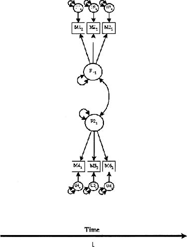
Figure 9.1: P-technique factor model.
![]()
and
![]()
where, as defined previously, y(t) is a p-variate observed time-series measured at time t (t = 1, 2, …, T), Λ is a p × k matrix of factor loadings, f (t – w), (t = 1, 2, …, T; w = 0, 1, 2, …s) is a k-variate time-series of (unobserved) factor scores w occasions prior to occasion t, u(t) is a p-variate time-series of unique parts of the observed scores that may have an auto-correlational but (for simplicity here) no cross-correlational structure, Bk is a weight matrix with element βkij in general reflecting the magnitude of influence of the ith factor from k occasions earlier on the current value of the jth factor, and v(t) is a disturbance term signifying concurrent contributions to the factor scores that are not part of the direct autoregressive structure.
By substitution we have
![]()
As noted previously, for the purposes of this discussion, βkij= 0 for i ≠ j (no cross-regressions). Equation 9.4 mandates that the influence of prior factor scores on the observed variables at time t is mediated through a given Bk. Precluding earlier factor scores from directly influencing later variable scores is a key point of difference between the DAFS model and that by Molenaar (1985) presented subsequently.
The distinguishing features of the DAFS model are (a) the factor loadings are invariant with respect to amount of lag (only one Λ is defined in the model), (b) possible autocorrelational structure in the common factor scores, and (c) possible autocorrelational structure in the uniquenesses of the variables. Thus, in this model the influence of the factor on the observed variables follows the same pattern regardless of the amount of lag, but the magnitude of the influence is diminished (or possibly enhanced) with increasing lag. For example, an extreme score on a factor at a given occasion would tend to produce an extreme score on a highly loaded variable on that occasion. For the score on that same observed variable one occasion later, however, that extreme factor score’s influence might be effectively diminished by a weight, say .5. Suppose the value of .5 held for all lags of one occasion. Then the effects of a lag of two occasions ought to be representable by a weighting of .5 × .5 = .25. Indeed, the invariance of the scaling weights across different amounts of lag is a statistically testable proposition.
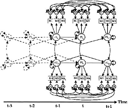
Figure 9.2: Direct autoregressive factor score (DAFS) model. An alternative representation involves replacing the variance on the common factors (circles labeled with F’s) with another circle representing an unmeasured innovation with a loading of unity and a variance of u. The more compact path modeling notation used here is consistent with that of Horn and McArdle (1980; p. 521).
To reiterate, in the DAFS model, the effect of yesterday’s factor score on today’s observed scores is mediated both by the level of time-related dependency residing in the factor scores and the elapsed time (number of lags). Although for many applications a simple autoregressive model would seem appropriate, in the case of strong delayed effects, for example, the data would be better accounted for by a large scaling value placed on the factor scores at some prior occasion of measurement. This does not necessarily pose a problem for the estimation of the model parameters unless there are insufficient degrees of freedom due to an excessive number of free parameters in the model.
Note that the model as estimated applies to the entire time-series. A lag of 2 applies equally to occasions 1 versus 3 and occasions 101 versus 103. Therefore, unique occurrences (e.g., a one-time “sleeper effect” such as an occurrence at occasion 5 having an influence on the organism at occasion 50) are “errors” in regard to both this model and that of Molenaar presented subsequently.
White Noise Factor Score Model (WNFS)
An early version of a WNFS model was presented by Geweke and Singleton (1981). Molenaar’s (1985, 1994; see also Hershberger et al., 1996; Wood & Brown, 1994) proposal for fitting the common factor model to multivariate time-series data-dynamic factor analysis involved allowing earlier factor scores to influence directly later values of the manifest variables. Thus, today’s observed scores are influenced both by today’s factor scores and by yesterday’s factor scores. To identify the time series of η(t) within the estimation framework he was using, Molenaar specified the common factor scores as a “white noise” time series. In general, other specifications could be used for the purpose of identification.
Molenaar’s specification can be represented in the following way
![]()
where y(t) is a p-variate observed time-series measured at time t(t=1,2,…,T), and η(t) is a k-variate time-series of (unobserved) factor scores at time t, є(t) is a vector of uniqueness at time t, and Λ(s) is a p × k matrix of factor loadings at lag s. Note that, in contrast to the DAFS model, in the specification of the WNFS model Λ carries a lag identifier e.g., Λ(1). The WNFS model is shown graphically in Figure 9.3. Distinguishing features of the WNFS model include (a) the factor loadings (regression-like weights that link observed variables to factors) differ according to the amount of lag, (b) as was noted above, instead of possible autocorrelational structure in the common factor scores over time, they are assumed to behave as “white noise,” and (c) possible autocorrelational structure in the uniquenesses of the variables. In this model, the current value of an observed variable is jointly influenced by today’s factor scores, yesterday’s factor scores, etc., today’s uniquenesses, and, possibly, yesterday’s specificity. Thus, the WNFS model represents such time-defined patterns of influence of factors on variables as decay, latency, and so on, via differences in the magnitude of the factor’s loadings on the variables as a function of time (lag).
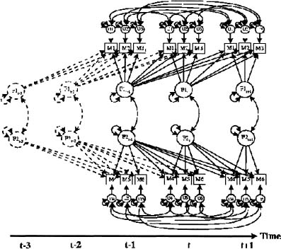
Figure 9.3: White noise factor score (WNFS) model.
Differences of the Two Models
In the previous section, the essential nature of the two model specifications under consideration was presented. The purpose of this section is to compare these two specifications for modeling multivariate time-series at the conceptual level. A more technical comparison and examination of the differences between the two models is provided at the end of the chapter in the Technical Appendix A.
Table 9.1
Comparison of Model Elements: Summary
| Elements | WNFS Model | DAFS Model |
| Factor loadings | Vary with amount of lag | Invariant with amount of lag |
| Factor Correlations | Can be correlated within lags but no across lags | Can be correlated within lags and across lags |
| Unique parts | Uncorrelated across variables but may have autoregressive character | Uncorrelated across variables but may have autoregressive character |
For easy reference, the similarities and differences of the two specifications are summarized in Table 9.1.
The two models differ fundamentally in the presumed nature of the common factors—especially the nature of the loading patterns at different lags—and thus represent process in distinctly different ways within the constraints dictated by the common factor model. Both models allow for a representation of continuity despite changes over time—a key feature of process—but the mechanisms by which factors drive variables, however, are notably different in the two model specifications.
The basic differences between the two models can be illustrated substantively, using state of food deprivation as the underlying condition (factor) that drives two measurable variables—blood sugar level and self-reported feelings of hunger. An appropriate time frame to consider here is hours instead of days or weeks. According to the DAFS model, current blood sugar level and self-reported hunger level are directly dependent on one’s current state of deprivation. Blood sugar level and self-reported hunger level an hour ago were dependent on the state of deprivation an hour ago in exactly the same way that current blood sugar level and self-reported hunger level are dependent on current deprivation state. To the extent that deprivation state an hour ago influences current deprivation state, deprivation state an hour ago also influences current blood sugar and self-reported hunger levels.
According to the WNFS model, current blood sugar level and self-reported hunger level are dependent both on current deprivation state and deprivation state an hour ago. Suppose the individual ate one half hour ago, thus attenuating the relationship between current deprivation state and deprivation state that held an hour ago. Given the WNFS specification, deprivation state an hour ago can have some lingering inuence on cation, deprivation state an hour ago can have some lingering inuence on blood sugar level, self-reported hunger level, or both. By contrast, given the DAFS specification, deprivation state an hour ago will influence both current blood sugar and self-reported hunger levels in an amount inversely proportional to the amount of attenuation in the relationship between current deprivation state and that of an hour ago. For example, if, after eating, blood sugar level and self-reported hunger level return to “baseline” at different rates, the WNFS model can represent the situation more flexibly but, as will be noted subsequently, the increased flexibility may have an accompanying cost of fewer degrees of freedom for evaluating model fit to the data.
Fitting the WNFS and DAFS Models to Data
To provide some concrete guidance for readers who would like to fit either or both the WNFS and DAFS models to data, we now illustrate a set of procedures by which this can be done. The data to which the two models will be fitted for this demonstration purpose were published originally by Lebo and Nesselroade (1978).2 The subset of the Lebo data used here consists of repeated measurements of one subject who rated her moods daily on a variety of adjective rating scales. A series of 103 days of reports on six scales was selected for these analyses: active, lively, and peppy to define an energy factor and sluggish, tired, and weary to define a fatigue factor. The correlations among these six variables are presented for lag 0, lag 1, and lag 2 in Table 9.2.
Estimating the Model Parameters
Following McArdle (1982), Molenaar (1985), and Wood and Brown (1994), the models were specified and their parameters estimated using LISREL 8 (Jöreskog & Sörbom, 1993). To incorporate the lagged information that is needed to estimate the model parameters in the form of a symmetric matrix for input to LISREL 8, a block-Toeplitz matrix as shown in Figure 9.4 was constructed from the data described earlier (for more details on block-Toeplitz matrices see Wood & Brown, 1994 and Nesselroade & Molenaar, 1999). The submatrices comprising the block-Toeplitz matrix were constructed individually by lagging the observed data on themselves by the appropriate number of lags. For example, the correlation for x lagging y by one lag was obtained by pairing observation xi2 with observation yi1, xi3 with yi2,…, and xiT–1 with yiT. The correlation for y lagging x by one lag was obtained by pairing observation yi2 with observation xi1, yi3 with xi2, … and yiT–1 with xiT. Obviously, at lag 1, the last observation of the lead variable and the first observation of the lagging variable are unmatched, so there is a consequent decrease in the functional N on which the correlation is based. Additional sample size is lost with the taking of additional lags. Moreover, the lagged correlation matrices are not symmetric because the correlation between x and y when y leads x is most likely different from the correlation between x and y when x leads y.
Table 9.2
Correlations Among Scales for Lags 0, 1, and 2
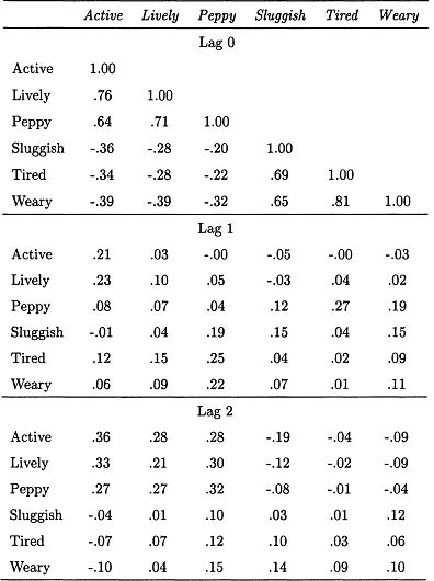
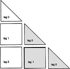
Figure 9.4: Schematized block-Toeplitz, lagged covariance matrix of Lags 0, 1, and 2.
To fit either of these two models using programs such as LISREL 8, the input covariance matrix must be symmetric. Therefore, in order to include the asymmetry of the lagged portions of the covariance matrix yet produce a symmetric matrix to be fitted, the block-Toeplitz matrix exhibits considerable redundancy as shown in Figure 9.4. To cope with the “false” degrees of freedom generated by the redundancy of the constructed matrix, the portions of the block-Toeplitz lagged covariance matrix shown as lightly shaded are estimated as free parameters in the model. Only some (or all, for the 0, 1, 2 lag model) of the left-most column blocks are actually fitted by the various models.
The general strategy followed was to fit the DAFS and WNFS models3 as they are represented in Figures 9.2 and 9.3 to the data of Table 9.2. This means that, in the lag 2 situation, the DAFS model allows for one factor to influence the score on another from both one and two occasions earlier. The lag 2 WNFS model allows for an observed variable to be influenced by a factor concurrently and from one and two occasions earlier. Both models were specified to have the same uniqueness structure, that shown in Figures 9.2 and 9.3.
The models were fitted to the full, lag 2 covariance matrix (see bottom panel of Figure 9.5). Note that, if one were to fit this 2-lag matrix with models of fewer lags of factors on variables than 2, some blocks of the covariance matrix might not be fitted at all. Figure 9.5 gives one illustration of which portions of the lagged covariance matrix might be fitted by each of three models (lag 0, lag 1, and lag 2). To illustrate, consider the P-technique model situation shown in panel a of Figure 9.5. One of the major criticisms of P-technique factor analysis has been that it ignores auto and cross-correlation in the data. As panel a shows, only the lag-0 information is accounted for by the model. To the extent that there is statistically significant information in the lagged portions of the block-Toeplitz matrix, it is ignored by the P-technique model. Alternative specifications one might use include “forcing” the lagged portions of the left-most column blocks to be zero versus “freeing” them as was done in our demonstration case with the elements in the lightly shaded portions of Figure 9.5.
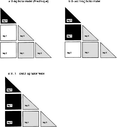
Figure 9.5: Schematized block-Toeplitz, lagged covariance matrix of Lags 0, 1, and 2, showing which lagged covariances are deliberately not fitted by the models (light shading) and which lagged covariances are forced to a value of zero by the models (unshaded).
To fit the DAFS model, we used the WNFS model specification to which we added several constraints.4 The first-order autoregressive effects were estimated by constraining the lag 1 factor loadings to Λ(1) = B1 · Λ(0) (see Technical Appendix A). The second-order autoregressive effects were estimated by constraining the lag 2 loadings to Λ(2) = ![]() · B2 · Λ(0). By constraining the lagged factor loadings, we were able to impose stationarity on the solution by estimating a disturbance on the concurrent factor (which was then the total variance at each lag). Because the autoregressive components were actually estimated by constraining the lagged loadings instead of as direct paths between the lagged factors, there was no “residual” component in the variance estimates of the lagged factors (see Technical Appendix A). An alternative specification would be to estimate the direct effects of the lagged factors on each other with regressionlike weights from factor to factor. Under that specification, the variance or residual variance on each lagged factor would be constrained so that the total variance at each lag was the same (to achieve stationarity). We did not use such a specification because we found that LISREL 8 was better able to handle the constraints on the loadings. Either procedure requires that the user observe the rules of path analysis (or the matrix equivalent) to specify the direct and indirect effects for each component in the model. For example, the lag 2 loading represents a lag 2 direct effect plus an indirect effect composed of the product of the lag 1 effects. Thus, when constraining the lag 2 loadings, both of these components were used to define the lag 2 loading. Finally, as indicated earlier, in the interest of keeping the model simple, cross-factor regressions were not estimated. Such estimations can be made by adding additional constraints on lagged loadings.
· B2 · Λ(0). By constraining the lagged factor loadings, we were able to impose stationarity on the solution by estimating a disturbance on the concurrent factor (which was then the total variance at each lag). Because the autoregressive components were actually estimated by constraining the lagged loadings instead of as direct paths between the lagged factors, there was no “residual” component in the variance estimates of the lagged factors (see Technical Appendix A). An alternative specification would be to estimate the direct effects of the lagged factors on each other with regressionlike weights from factor to factor. Under that specification, the variance or residual variance on each lagged factor would be constrained so that the total variance at each lag was the same (to achieve stationarity). We did not use such a specification because we found that LISREL 8 was better able to handle the constraints on the loadings. Either procedure requires that the user observe the rules of path analysis (or the matrix equivalent) to specify the direct and indirect effects for each component in the model. For example, the lag 2 loading represents a lag 2 direct effect plus an indirect effect composed of the product of the lag 1 effects. Thus, when constraining the lag 2 loadings, both of these components were used to define the lag 2 loading. Finally, as indicated earlier, in the interest of keeping the model simple, cross-factor regressions were not estimated. Such estimations can be made by adding additional constraints on lagged loadings.
Results
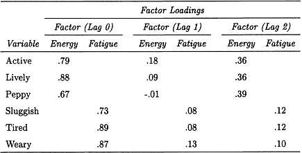
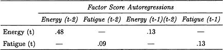
To complete the illustration of fitting the WNFS and DAFS models to the subject’s data for lags of 0, 1, and 2, summary information is presented in Tables 9.3 and 9.4, respectively. Both models appear to fit the data adequately but, more important for our purposes, the distinct features of both models are clearly manifested in the outcomes. Neither the Fatigue factor nor the manifest variables it loads appear to exhibit autoregressive characteristics. This is not the case for Energy and its indicators, however. The WNFS model (Table 9.3) shows the autoregressive nature of the system with statistically significant lagged factor loadings, whereas the DAFS model (Table 9.4) displays the analogous information by the statistically significant prediction of the Energy factor scores at time t by their values at time t – 2. Highly similar values were estimated for the correlation between Energy and Fatigue within occasions in the two cases (-.37 and -.38). Although not presented here, the patterns of autocorrelations of the unique parts were also very similar in the two cases.
Table 9.3
WNFS Model Fit Outcomes (χ2 = 77.54; df = 56; RMSEA = .054; probability of close fit = .4)
Note: Energy and Fatigue factors are correlated -.37 within occasions.
DISCUSSION
One of the general benefits for the study of behavior of applying the WNFS and DAFS models to multivariate time series to represent process is the forced confrontation with having to define process explicitly. The term process is widely used and easy to say but, to rigorously fit and evaluate different representations, it has to be given a specific operational expression. By means of the WNFS and the DAFS models and within the constraints of the common factor model we have rendered process operational in two distinctive ways. The WNFS and DAFS models rest on markedly different interpretations of the nature of the factor variables. In the WNFS model, the factors themselves represent unobserved, unpredictable “shocks” to the system of manifest variables. Thus, process in this case is defined in terms of the systematic, lagged effects on the manifest variables. In the DAFS model, the factor scores can be relatively stable and predictable with changes in those factor scores caused by unobserved, unpredictable “shocks” acting on the factors. The manifest variables in the DAFS model are multiple indicators of the underlying processes represented by the factors.
Some readers will no doubt question the efficacy of the WNFS and DAFS models for representing process, and it is clear that many other possibilities exist, should an investigator wish to make use of them. Nevertheless, the specifications we have presented have behind them a halfcentury of concern with representing process in quantitative models by means of multivariate, latent variable specifications. Fitting these models to data underscores the level of precision that an investigator must be willing to provide to model process in quantitatively rigorous terms. The results of these model-fitting exercises hint at some of the gains that can accrue when one does so.
Table 9.4
DAFS Model Fit Outcomes (χ2 = 87.19; df = 64; RMSEA = .046; probability of close fit = .55)
| Factor Loadings | ||
| Variable | Energy | Fatigue |
| Active | .77 | |
| Lively | .86 | |
| Peppy | .67 | |
| Sluggish | .71 | |
| Tired | .86 | |
| Weary | .87 | |
Note: Energy and Fatigue factors are correlated -.38 within occasions.
Under the constraints outlined in Technical Appendix A, the DAFS model is a restrictive version of the WNFS model, which, due to additional constraints on the factor structure, may not fit the time-series data as well. For a given problem size (number of variables, number of factors, and number of lags) and three or more indicators per factor, the DAFS model generally has fewer parameters than the WNFS model, the exact numbers depending on the actual specifications. This can also be seen by counting the paths among latent variables in Figures 9.2 and 9.3. In cases where the data meet the proportionality constraints of the DAFS model (see Technical Appendix A), the DAFS specification will have smaller error of estimation because it has more degrees of freedom. Thus, the flexibility of the WNFS model to portray differentials in the rates at which variables change in response to changes in the factor scores (a situation that violates the proportionality constraints) costs degrees of freedom. The cost may well be worth it, however, in cases where changes in variables loaded by the same factor show quite different lag patterns. As a “restrictive” version of the more general WNFS model, the DAFS model is scientifically very useful. This restrictive relationship among alternative multivariate models parallels the mathematical basis and scientific use of a “common psychometric factor” model with behavioral genetics data (McArdle & Goldsmith, 1990).
Obviously many variations on the WNFS and DAFS models described previously are possible. One can argue that conceptually the two models represent very different notions of process and thus should not necessarily be seen merely as alternative models for fitting a given set of data. Nevertheless, to make this parallel application of the two models as informative as possible, we specified both of them in a way that highlighted their similarities. For example, we specified the same uniqueness structure for both models. If the two models account in a similar way for the same data, then the argument of parsimony would favor the model with the fewest parameters. If the two differ in the way they account for the same data, then the evaluation has to take into account the parsimony of the model as well as other features. Ultimately, it will be necessary to compare alternative specifications using many different kinds of data representing different kinds of processes if the further development and use of these models is to be maximally effective.
At a more specific level, the models of process we presented illlustrate how refinements and subtleties in representations can be evaluated within the context of a general quantitative model (e.g., the common factor model). We demonstrated the underlying kinship of what, on the surface, appear to be distinct representations of process information. By showing that one of the models is a more restrictive version of the other, one can enter the scientifically highly productive arena of testing and evaluating the appropriateness of substantively meaningful restrictions imposed on rigorous, quantitative models.
To illustrate some of the subtleties of the process modeling issues, consider the importance of being able to model differential rates of return to equilibrium of different manifest variables after some extraordinary event. Disparate temporal paths to the restoration of equilibrium would seem, at least on the surface, to favor the representational flexibility of the WNFS model. However, it is likely to be the case that the mechanism of self-report “smooths” differences in the rates of change (reported) at the manifest variable level, thus tending to favor the more parsimonious DAFS representation over the WNFS one. Thus, media of observation (self-report, ratings by others, objective performance measures), for instance, may well interact with the model specifications in the attempt to represent process at the latent variable level.
Neither the WNFS nor the DAFS model specification should be regarded as a “winner” in some modeling context. It is entirely possible that a DAFS model is a reasonable representation for factor 1 but not for factor 2, and so on. The choice between which one to fit should be made primarily out of substantive considerations. Thus, it is important to continue to explore alternative model specifications using data drawn from a variety of content domains.
Finally, it is our view that never before in the study of behavior has the time to focus on modeling process and change been so ripe (Nesselroade & Schmidt McCollam, 2000). Historically, we are at a confluence of several substantive and methodological influences that are drawing more and more attention to intraindividual variability phenomena (Nesselroade & Featherman, 1997). Success in capitalizing on this historical opportunity will rest heavily on our ability to proceed with precision and rigor as the cherished and familiar concepts called “processes” are rendered more operational.
TECHNICAL APPENDIX A. DIFFERENCES AND SIMILARITIES OF WNFS AND DAFS MODELS
To examine the WNFS and DAFS models at a somewhat more technical level, consider these simplified (first order lags only) equations
![]()
of the WNFS model and
![]()
![]()
of the DAFS model. A closer inspection of the relations between these two time series based factor models shows their equivalence under some constraints on the WNFS model. Starting with the DAFS model,
![]()
or
![]()
Rearranging terms, we have
![]()
By stationarity, f(t – 2) has a zero mean and the same variance as f (t). Redefining
Λ = Λ(0)
v(t) = η(t)
Λ· B = Λ(1)
u(t) = є(t)
yields
![]()
where q is a residual term = Λ · B2 · f (t – 2). The q term signifies an error of approximation random variable. Thus, for the WNFS and DAFS models to be equivalent, the pattern of first-order white noise factor loadings, Λ(1) is required to be “proportional” to Λ(0) [i.e., Λ(0) = Λ and Λ(1) = Λ · B = Λ(0) · B] and Λ · B2 · f (t – 2) must have a negligible covariance matrix.
Consider the second-order lag equations of the same two model specifications. The WNFS model for Lag-2 effects can be written as
![]()
and the DAFS model for lag-2 effects can be written as
![]()
and
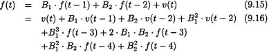
Combining the two terms involving v(t – 2) we have
Similar to the previous development,
Redifining
Λ = Λ (0)
v(t) = η(t)
Λ · B1 = Λ(1)
Λ · ![]() · B2 = Λ (2)
· B2 = Λ (2)
u(t) = є(t)
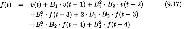
and substituting yields
![]()
where q, a residual term, represents
Λ[![]() . f(t-3) + 2 · B1 · B2 · f(t-3) +
. f(t-3) + 2 · B1 · B2 · f(t-3) + ![]() · B2 · f(t-4) +
· B2 · f(t-4) + ![]() · f(t-4)]
· f(t-4)]
This is the WNFS model with lags of 0, 1, and 2 plus the residual term.
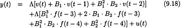
Thus, for the WNFS and DAFS models to be equivalent in the lag 2 case, the patterns of first- and second-order white noise factor loadings, Λ(1) and Λ(2), are required to be “proportional” to the autoregression weights, B1 and B2 [i.e., Λ(0) = Λ, Λ(1) = Λ · B1 = Λ(0) · B1, and Λ(2) = Λ · ![]() · B2 = Λ(0) ·
· B2 = Λ(0) · ![]() · B2and for Λ[
· B2and for Λ[ ![]() . f(t-3) + 2 · B1 · B2 · f(t-3) +
. f(t-3) + 2 · B1 · B2 · f(t-3) + ![]() · B2 · f(t-4) +
· B2 · f(t-4) + ![]() · f(t – 4)] to have a negligible covariance matrix. This process repeats in similar fashion for higher orders of lags.
· f(t – 4)] to have a negligible covariance matrix. This process repeats in similar fashion for higher orders of lags.
We return to Molenaar’s specification of the WNFS model (Equation 5) for further consideration.
y(t) = Λ(0)η(t) + Λ(1)η(t - 1) + … + Λ(s)η(t - s) + є(t)
The WNFS model is a general model for any time series data with a factor analytic structure when s = ∞. When the proportionality constraints described previously hold and Bs+1 is “approximately” a null matrix, the WNFS model “approximately” fits a time series with a DAFS structure. To the extent that the covariance matrices implied by the residual terms do not vanish, the lags of the WNFS model will tend to be greater than the order of the DAFS model.
TECHNICAL APPENDIX B. LISREL CODE FOR RUNNING WNFS AND DAFS MODELS
The WNFS MODEL-Lebo Data, 2 FACTORS, 0,1, and 2 LAGS
da ni = 18 no = 103 ma = km
km sy = lebo.dat
mo ny = 18 ne = 10 ly = fu, fi ps = sy, fi te = sy, fi be = fu, fi
LA
active0 lively0 peppy0 slugish0 tired0 weary0
active1 lively1 peppy1 slugish1 tired1 weary1
active2 lively2 peppy2 slugish2 tired2 weary2
LE
ENERGYO FATIGUEO ENERGY1 FATIGUE1 ENERGY2 FATIGUE2
ENERGY3 FATIGUE3 ENERGY4 FATIGUE4
!LAG 0 FACTOR LOADINGS
FR LY(1,1) LY(2,1) LY(3,1) LY(4,2) LY(5,2) LY(6,2)
EQ LY(1,1) LY(7,3) LY(13,5)
EQ LY(2,1) LY(8,3) LY(14,5)
EQ LY(3,1) LY(9,3) LY(15,5)
EQ LY(4,2) LY(10,4) LY(16,6)
EQ LY(5,2) LY(11,4) LY(17,6)
EQ LY(6,2) LY(12,4) LY(18,6)
!LAG 1 FACTOR LOADINGS
FR LY(1,3) LY(2,3) LY(3,3) LY(4,4) LY(5,4) LY(6,4)
EQ LY(1,3) LY(7,5) LY(13,7)
EQ LY(2,3) LY(8,5) LY(14,7)
EQ LY(3,3) LY(9,5) LY(15,7)
EQ LY(4,4) LY(10,6) LY(16,8)
EQ LY(5,4) LY(11,6) LY(17,8)
EQ LY(6,4) LY(12,6) LY(18,8)
FR LY(1,5) LY(2,5) LY(3,5) LY(4,6) LY(5,6) LY(6,6)
EQ LY(1,5) LY(7,7) LY(13,9)
EQ LY(2,5) LY(8,7) LY(14,9)
EQ LY(3,5) LY(9,7) LY(15,9)
EQ LY(4,6) LY(10,8) LY(16,10)
EQ LY(5,6) LY(11,8) LY(17,10)
EQ LY(6,6) LY(12,8) LY(18,10)
!UNIQUE VARIANCES AND COVARIANCES
FR TE(1,1) TE(2,2) TE(3,3) TE(4,4) TE(5,5) TE(6,6)
FR TE(7,1) TE(8,2) TE(9,3) TE(10,4) TE(11,5) TE(12,6)
FR TE(13,1) TE(14,2) TE(15,3) TE(16,4) TE(17,5) TE(18,6)
FR TE(7,7)
FR TE(8,7) TE(8,8)
FR TE(9,7) TE(9,8) TE(9,9)
FR TE(10,7) TE(10,8) TE(10,9) TE(10,10)
FR TE(11,7) TE(11,8) TE(11,9) TE(11,10) TE(11,11)
FR TE(12,7) TE(12,8) TE(12,9) TE(12,10) TE(12,11) TE(12,12)
FR FR TE(13, 13)
FR TE(14,13) TE(14,14)
FR TE(15,13) TE(15,14) TE(15, 15)
FR TE(16,13) TE(16,14) TE(16, 15) TE(16,16)
FR TE(17,13) TE(17,14) TE(17, 15) TE(17,16) TE(17,17)
FR TE(18,13) TE(18,14) TE(18, 15) TE(18,16) TE(18,17) TE(18,18)
FR TE(13,7) TE(13,8) TE(13,9) TE(13,10) TE(13,11) TE(13,12)
FR TE(14,7) TE(14,8) TE(14,9) TE(14,10) TE(14,11) TE(14,12)
FR TE(15,7) TE(15,8) TE(15,9) TE(15,10) TE(15,11) TE(15,12)
FR TE(16,7) TE(16,8) TE(16,9) TE(16,10) TE(16,11) TE(16,12)
FR TE(17,7) TE(17,8) TE(17,9) TE(17,10) TE(17,11) TE(17,12)
FR TE(18,7) TE(18,8) TE(18,9) TE(18,10) TE(18,11) TE(18,12)
!SCALING CONSTRAINTS
VA 1.0 PS(1,1) PS(3,3) PS(5,5) PS(7,7) PS(9,9)
VA 1.0 PS(2,2) PS(4,4) PS(6,6) PS(8,8) PS(10,10)
!FACTOR COVARIANCES
FR PS(2,1)
EQ PS(2,1) PS(4,3) PS(6,5) PS(8,7) PS(10,9)
ST 1.0 TE(1,1) TE(2,2) TE(3,3) TE(4,4) TE(5,5) TE(6,6)
ST 0.01 LY(1,1) LY(2,1) LY(3,1) LY(4,2) LY(5,2) LY(6,2)
ou me = ml xm ns so se tv ss nd = 2 it = 500 ad = off
The DAFS MODEL-Lebo Data, 2 FACTORS, 0,1, and 2 LAGS
da ni = 18 no = 103 ma = km
km sy fi = lebo.dat
mo ny = 18 ne = 10 ly = fu, fi ps = sy, fi te = sy, fi
LA
active0 lively0 peppy0 slugish0 tired0 weary0
active1 lively1 peppy1 slugish1 tired1 weary1
active2 lively2 peppy2 slugish2 tired2 weary2
LE
ENERGY0 FATIGUE0 ENERGY1 FATIGUE1 ENERGY2 FATIGUE2
ENERGY3 FATIGUE3 ENERGY4 FATIGUE4
!FACTOR LOADINGS
FR LY(1,1) LY(2,1) LY(3,1) LY(4,2) LY(5,2) LY(6,2)
EQ LY(1,1) LY(7,3) LY(13,5)
EQ LY(2,1) LY(8,3) LY(14,5)
EQ LY(3,1) LY(9,3) LY(15,5)
EQ LY(4,2) LY(10,4) LY(16,6)
EQ LY(5,2) LY(11,4) LY(17,6)
EQ LY(6,2) LY(12,4) LY(18,6)
!FACTOR LOADING CONSTRAINTS (TO DEAL WITH LAG 1)
FR LY(1,3) LY(2,3) LY(3,3) LY(4,4) LY(5,4) LY(6,4)
EQ LY(1,3) LY(7,5) LY(13,7)
EQ LY(2,3) LY(8,5) LY(14,7)
EQ LY(3,3) LY(9,5) LY(15,7)
EQ LY(4,4) LY(10,6) LY(16,8)
EQ LY(5,4) LY(11,6) LY(17,8)
EQ LY(6,4) LY(12,6) LY(18,8)
!FACTOR LOADING CONSTRAINTS (TO DEAL WITH LAG 2)
FR LY(1,5) LY(2,5) LY(3,5) LY(4,6) LY(5,6) LY(6,6)
EQ LY(1,5) LY(7,7) LY(13,9)
EQ LY(2,5) LY(8,7) LY(14,9)
EQ LY(3,5) LY(9,7) LY(15,9)
EQ LY(4,6) LY(10,8) LY(16,10)
EQ LY(5,6) LY(11,8) LY(17,10)
EQ LY(6,6) LY(12,8) LY(18,10)
!UNIQUE VARIANCES AND COVARIANCES
FR TE(1,1) TE(2,2) TE(3,3) TE(4,4) TE(5,5) TE(6,6)
FR TE(7,1) TE(8,2) TE(9,3) TE(10,4) TE(11,5) TE(12,6)
FR TE(13,1) TE(14,2) TE(15,3) TE(16,4) TE(17,5) TE(18,6)
FR TE(7,7)
FR TE(8,7) TE(8,8)
FR TE(9,7) TE(9,8) TE(9,9)
FR TE(10,7) TE(10,8) TE(10,9) TE(10,10)
FR TE(11,7) TE(11,8) TE(11,9) TE(11,10) TE(11,11)
FR TE(12,7) TE(12,8) TE(12,9) TE(12,10) TE(12,11) TE(12,12)
FR TE(13,13)
FR TE(14,13) TE(14,14)
FR TE(15,13) TE(15,14) TE(15,15)
FR TE(16,13) TE(16,14) TE(16,15) TE(16,16)
FR TE(17,13) TE(17,14) TE(17, 15) TE(17,16) TE(17,17)
FR TE(18,13) TE(18,14) TE(18, 15) TE(18,16) TE(18,17) TE(18,18)
FR TE(13,7) TE(13,8) TE(13,9) TE(13,10) TE(13,11) TE(13,12)
FR TE(14,7) TE(14,8) TE(14,9) TE(14,10) TE(14,11) TE(14,12)
FR TE(15,7) TE(15,8) TE(15,9) TE(15,10) TE(15,11) TE(15,12)
FR TE(16,7) TE(16,8) TE(16,9) TE(16,10) TE(16,11) TE(16,12)
FR TE(17,7) TE(17,8) TE(17,9) TE(17,10) TE(17,11) TE(17,12)
FR TE(18,7) TE(18,8) TE(18,9) TE(18,10) TE(18,11) TE(18,12)
!SCALING CONSTRAINTS
VA 1.0 PS(1,1) PS(3,3) PS(5,5) PS(7,7) PS(9,9)
VA 1.0 PS(2,2) PS(4,4) PS(6,6) PS(8,8) PS(10,10)
!FACTOR COVARIANCES
FR PS(2,1)
EQ PS(2,1) PS(4,3) PS(6,5) PS(8,7) PS(10,9)
ST 1.0 TE(1,1) TE(2,2) TE(3,3) TE(4,4) TE(5,5) TE(6,6)
ST 0.01 LY(1,1) LY(2,1) LY(3,1) LY(4,2) LY(5,2) LY(6,2)
!Factor One
!First-Order Autoregression F1[t-1] → F1[t]
FR PA(1)
CO LY(1,3) = LY(1,1)∗PA(1)
CO LY(2,3) = LY(2,1)∗PA(1)
CO LY(3,3) = LY(3,1)∗PA(1)
EQ LY(1,3) LY(7,5) LY(13,7)
EQ LY(2,3) LY(8,5) LY(14,7)
EQ LY(3,3) LY(9,5) LY(15,7)
!Second-Order Autoregression F1[t-2] → F1[t]
FR PA(3)
CO LY(1,5) = LY(1,1)∗PA(1)∗PA(1) +LY(1,1)∗PA(3)
CO LY(2,5) = LY(2,1)∗PA(1)∗PA(1) +LY(2,1)∗PA(3)
CO LY(3,5) = LY(3,1)∗PA(1)∗PA(1) +LY(3,1)∗PA(3)
EQ LY(1,5) LY(7,7) LY(13,9)
EQ LY(2,5) LY(8,7) LY(14,9)
EQ LY(3,5) LY(9,7) LY(15,9)
!Factor Two
!First-Order Autoregression F2[t-1] → F2[t]
FR PA(2)
CO LY(4,4) = LY(4,2)∗PA(2)
CO LY(5,4) = LY(5,2)∗PA(2)
CO LY(6,4) = LY(6,2)∗PA(2)
EQ LY(4,4) LY(10,6) LY(16,8)
EQ LY(5,4) LY(11,6) LY(17,8)
EQ LY(6,4) LY(12,6) LY(18,8)
!Second-Order Autoregression F2[t-2] → F2[t]
FR PA(4)
CO LY(4,6) = LY(4,2)∗PA(2)∗PA(2) +LY(4,2)∗PA(4)
CO LY(5,6) = LY(5,2)∗PA(2)∗PA(2) +LY(5,2)∗PA(4)
CO LY(6,6) = LY(6,2)∗PA(2)∗PA(2) +LY(6,2)∗PA(4)
EQ LY(4,6) LY(10,8) LY(16,10)
EQ LY(5,6) LY(11,8) LY(17,10)
EQ LY(6,6) LY(12,8) LY(18,10)
!Starting Values for all regression parameters
ST -.1 PA(1) PA(2) PA(3) PA(4)
ou me = ml xm ns so se tv ss nd = 2 it = 500 ad = off
ACKNOWLEDGMENTS
This work was supported by the Institute for Developmental and Health Research Methodology at the University of Virginia. An earlier version was presented at the Annual Meeting of the American Psychological Association, San Francisco, August, 1997. This final manuscript was completed while JRN was a Senior Guest Scientist at the Max Planck Institute for Human Development, Berlin, Germany. The authors acknowledge with gratitude the helpful comments of Michael Browne and Peter C. M. Molenaar on an earlier version of this chapter.
REFERENCES
Anderson, T. W. (1963). The use of factor analysis in the statistical analysis of multiple time series. Psychometrika, 28, 1–24.
Baltes, P. B., Reese, H. W., & Nesselroade, J. R. (1977). Life-span developmental psychology: Introduction to research methods. Monterey, CA: Brookes/Cole.
Bereiter, C. (1963). Some persisting dilemmas in the measurement of change. In C. W. Harris (Ed.), Problems in measuring change. Madison: University of Wisconsin Press.
Cattell, R. B. (1952). Factor analysis. New York: Harper.
Cattell, R. B. (1957). Personality and motivation structure and measurement. New York: World.
Cattell, R. B. (1961). Factor analysis. New York: Harpe.
Cattell, R. B. (1963a). The interaction of hereditary and environmental influences. The British Journal of Statistical Psychology, 16, 191–210.
Cattell, R. B. (1963b). The structuring of change by p-technique and incremental r-technique. In C. W. Harris (Ed.), Problems in measuring change (p. 167–198). Madison: University of Wisconsin Press.
Cattell, R. B. (1996). Patterns of change: Measurement in relation to state dimension, trait change, lability, and process concepts. In R. B. Cattell (Ed.), Handbook of multivariate experimental psychology (p. 355–402). Chicago, IL: Rand McNally.
Cattell, R. B., Cattell, A. K. S., & Rhymer, R. M. (1947). P-technique demonstrated in determining psychophysical source traits in a normal individual. Psychometrika, 12, 267–288.
Eizenman, D. R., Nesselroade, J. R., Featherman, D. L., & Rowe, J. W. (1997). Intra-individual variability in perceved control in an elderly sample: The MacArthur successful aging studies. Psychology and Aging, 12, 489–502.
Engle, R., & Watson, M. (1981). A one-factor multivariate time series model of metropolitan wage rates. Journal of American Statistical Association, 76, 774–781.
Fiske, D. W., & Maddi, S. R. (Eds.). (1961). Functions of varied experience. Homewood, IL: Dorsey Press.
Fiske, D. W., & Rice, L. (1955). Intra-individual response variability. Psychological Bulletin, 52, 217–250.
Flugel, J. C. (1928). Practice, fatigue, and oscillation. British Journal of Psychology, 4, 1–92.
Geweke, J. F., & Singleton, K. J. (1981). Maximum likelihood “confirmatory” factor analysis of economic time series. International Economic Review, 22, 37–54.
Hershberger, S. L., Molenaaar, P. C., & Corneal, S. E. (1996). A hierarchy of univariate and multivariate time series models. In G. A. Marcoulides & R. E. Schumacker (Eds.), Advanced structural equation modeling: Issues and techniques (p. 159–194). Mahwah, NJ: Lawrence Erlbaum Associates.
Holtzman, W. H. (1963). Statistical models for the study of change in the single case. In C. W. Harris (Ed.), Problems in measuring change (p. 199–211). Madison: University of Wisconsin Press.
Horn, J. L. (1972). State, trait, and change dimensions of intelligence. The British Journal of Educational Psychology, 42, 159–185.
Horn, J. L., & McArdle, J. J. (1980). Perspectives on mathematical and statistical model building (masmob) in research on aging. In L. Poon (Ed.), Aging in the 1980’s: Psychological issues (p. 203–541). Washington, DC: American Psychological Association.
Hundleby, J. D., Pawlik, K., & Cattell, R. B. (1965). Personality factors in objective test devices. San Diego, CA: R. Knapp.
Jones, C. J., & Nesselroade, J. R. (1990). Multivariate, replicated, single-subject designs and p-techniques factor analysis: A selective review of the literature. Experimental Aging Research, 16, 171–183.
Jones, K. (1991). The application of time series methods to moderate span longitudinal data. In L.M. Collins & J. L. Horn (Eds.), Best methods for the analysis of change: Recent advances, unanswered questions, future directions (p. 75–87). Washington, DC: American Psychological Association.
Jöreskog, K. G., & Sörbom, D. (1993). Lisrel 8: Structural equation modeling with the simplis command language. Hillsdale, NJ: Lawrence Erlbaum Associates.
Kenny, D. A., & Zautra, A. (1995). The trait-state error model for multiwave data. Journal of Consulting and Clinical Psychology, 63, 52–59.
Kim, J. E., Nesselroade, J. R., & Featherman, D. L. (1996). The state component in self-reported world views and religious beliefs in older adults: The MacArthur successful aging studies. Psychology and Aging, 11, 396–407.
Larsen, R. J. (1987). The stability of mood variability: A spectral analysis approach to daily mood assessments. Journal of Personality and Social Psychology, 52, 1195–1204.
Lebo, M. A., & Nesselroade, J. R. (1978). Intraindividual differences dimensions of mood change during pregnancy identified by five p-technique factor analyses. Journal of Research in Personality, 12, 205–224.
Luborsky, L., & Mintz, J. (1972). The contribution of p-technique to personality, psychotherapy, and psychosomatic research. In R. M. Dreger (Ed.), Multivariate personality research: Contributions to the understanding of personality in honor of Raymond B. Cattell (p. 387–410). Baton Rouge, LA: Claitor’s Publishing Division.
Magnusson, D. (1997). The logic and implications of a person approach. In R. B. Cairns, L. R. Bergman, & J. Kagan (Eds.), The individual as a focus in developmental research. New York: Sage.
McArdle, J. J. (1982). Structural equation modeling of an individual system: Preliminary results from “a case study in episodic alcoholism”. (Unpublished manuscript, Department of Psychology, University of Denver)
McArdle, J. J., & Goldsmith, H. H. (1990). Some alternative structural equation models for multivariate biometric analyses. Behavior Genetics, 20, 569–608.
Molenaar, P. C. M. (1985). A dynamic factor model for the analysis of multivariate time series. Psychometrika, 50, 181–202.
Molenaar, P. C. M. (1994). Dynamic latent variable models in developmental psychology. In A. von Eye & C. C. Clogg (Eds.), Latent variables analysis: Applications for developmental research (p. 155–180). Newbury Park, CA: Sage.
Nesselroade, J. R., & Boker, S. M. (1994). Assessing constancy and change. In T. Heatherton & J. Weinberger (Eds.), Can personality change? (p. 121–147). Washington, DC: American Psychological Association.
Nesselroade, J. R., & Featherman, D. L. (1997). Establishing a reference frame against which to chart age-related change. In M. A. Hardy (Ed.), Studying aging and social change: Conceptual and methodological issues (p. 191–205). Thousand Oaks, CA: Sage.
Nesselroade, J. R., & Ford, D. H. (1985). P-technique comes of age: Multivariate, replicated, single-subject designs for research on older adults. Research on Aging, 7, 46–80.
Nesselroade, J. R., & Molenaar, P. C. M. (1999). Pooling lagged covariance structures based on short, multivariate time-series for dynamic factor analysis. In R. H. Hoyle (Ed.), Statistical strategies for small sample research (p. 224–251). Newbury Park, CA: Sage.
Nesselroade, J. R., & Schmidt McCollam, K. M. (2000). Putting the process in developmental processes. International Journal for the Study of Behavioral Development, 24, 295–300.
Singer, J. L., & Singer, D. G. (1972). Personality. Annual Review of Psychology, 23, 375–412.
Steyer, R., Ferring, D., & Schmitt, M. (1992). States and traits in psychological assessment. European Journal of Psychological Assessment, 8, 79–98.
Valsiner, J. (1984). Two alternative epistemological frameworks in psychology: The typological and variational modes of thinking. The Journal of Mind and Behavior, 5, 449–470.
Wessman, A. E., & Ricks, D. F. (1966). Mood and personality. New York: Holt, Rinehart, and Winston.
Wood, P., & Brown, D. (1994). The study of intraindividual differences by means of dynamic factor models: Rationale, implementation, and interpretation. Psychological Bulletin, 116, 166–186.
Woodrow, H. (1932). Quotidian variability. Psychological Review, 39, 245–256.
Woodrow, H. (1945). Intelligence and improvement in school subjects. Journal of Educational Psychology, 36, 155–166.
Zevon, M., & Tellegen, A. (1982). The structure of mood change: Idiographic/nomothetic analysis. Journal of Personality and Social Psychology, 43, 111–122.
__________________________________
1Although it is possible to include them as parameters in the model, to simplify this presentation, cross-correlations among the common factors have been omitted.
2We are grateful to Dr. Michael A. Lebo for permission to use these data.
3The lisrel code that was used is presented in Technical Appendix B.
4In his 1985 paper, Molenaar indicated that what is here referred to as the DAFS model is a state-space model and hence is a specific version of his dynamic factor model. Molenaar went on to indicate that if the loadings in a dynamic factor model are only nonzero at lag zero, the dynamic factor model reduces to a generalized state-space model and proved that in that case the covariance function of the latent factor series is identified and thus can be uniquely estimated.