
Every Mudbox sculpture starts out as a polygon mesh. You could start with one of the 10 provided with Mudbox—for example, the sphere that you sculpted into the egg in Chapter 1, "Getting Your Feet in the Mud: The Basics of the Mudbox Production Pipeline." The sculpture could also start out as a full mesh modeled in a 3D application such as Maya, 3ds Max, Softimage, or Modo. An example of this is the model of Bertie that you worked on in Chapter 3, "Detail-Sculpting an Imported Model," and Chapter 4, "Painting and Texturing an Imported Model." Bertie was modeled, rigged, and posed in Maya and brought into Mudbox for detail sculpting and painting. You could start with a downloaded base mesh from the Mudbox Community on the AREA or from many online websites, for free or for a nominal price. Finally, a model can be brought in as a 3D scan from a 3D scanner, which is a device that generates a polygon mesh from a physical 3D object. Just as 2D scanners, which are now very inexpensive and common, are used to scan pictures and text, 3D scanners are used to scan 3D objects.
In this chapter, you will go through the benefits and limitations of 3D scan data. You will learn how you can use Mudbox's sculpting tools to overcome these limitations and clean up the 3D scans. You can then generate displacement maps from the scan data and map them to usable topology.
This chapter includes the following topics:
Understanding the benefits and challenges of 3D scan data
Using 3D scanners
Reviewing scan data import considerations
Importing 3D scan data and re-topologizing in Mudbox
Three-dimensional scanning is a quick, simple, and fairly inexpensive process used to generate near-perfect likenesses of people and props. When CG models are required as stunt doubles for real actors in movies, advertisements, and characters in video games, it is critical to have a believable likeness. The data generated by a 3D scan is indispensible for creating models that represent that required likeness.
Although the scan process is quick, simple, and fairly inexpensive, in almost all cases, the generated 3D scan data does not replace the needed 3D model. For example, the basketball player or film/TV actor model generated by the 3D scan is not the model animators will use to animate the basketball player for a video game or the actor for an impossible stunt.
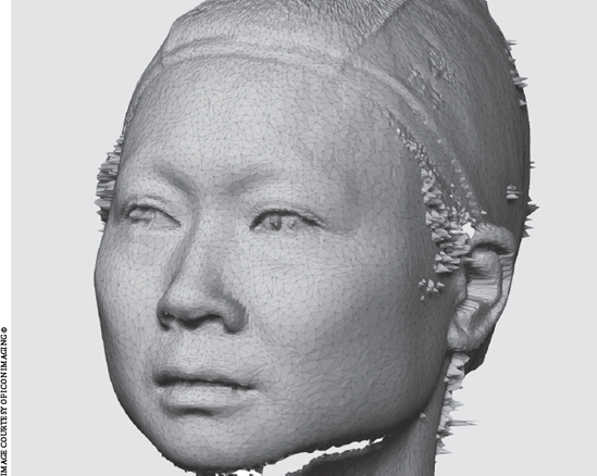
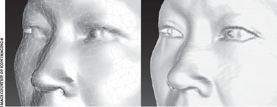
There are several reasons for this. One is that 3D scanners sample points on a body's surface to create a likeness of the shape without giving any consideration to topology or polygon count. The data from 3D scans is usually in the order of millions of triangles arranged in a completely random pattern to represent the surface of the scanned subject (Figure 7.1). Even though the representation is perfect, the makeup of that representation is not.
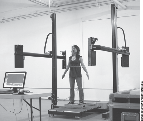
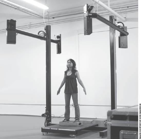
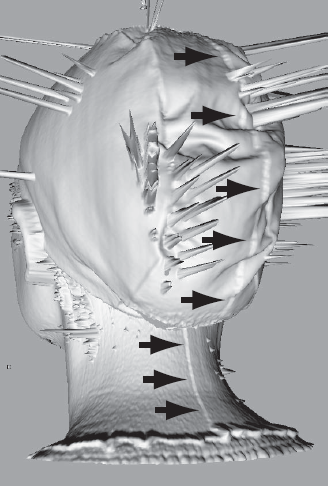
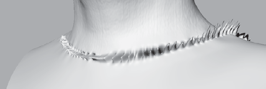
Yet another challenge is that even if the most skillful scan artists use the best scanners to scan a model that poses for the scan, they would still get a resulting 3D mesh that had anomalies. Just the slightest movement of a human subject—even ones who are able to stand relatively still during the scan process (which entails having multiple scanners moving around the person and scanning bands of points on the surface of the body)—always generates undesirable surface anomalies, such as ripples or stretching (Figure 7.2).
Three-dimensional scanners also have difficulty working around occluded areas on the surface that fold over or have holes; we see this with 3D scan data of ears and areas under the chin. This is because blind spots exist that the 3D scanner cannot scan. It is also difficult to scan details such as hair or surfaces that are transparent or reflective. These result in anomalies and holes on the resulting 3D scan (Figure 7.3).
Data from a 3D scan can be used with minimal processing only when the object is to be rendered in a stationary position. Even in these cases, the model still needs to be cleaned up of 3D scan anomalies and optimized to reduce the polygon count so that rendering engines can process the data and render the scene in a reasonable time frame.
On the flip side, it would take an extremely talented modeler and sculptor to create a model from scratch to match the precision and likeness of a well-recognized person that our discerning eyes will accept. This talent is a limited and expensive resource. In addition, the sheer volume of models needed for production cycles of games, movies, and advertisements is getting greater while the time frame within which they are needed is getting shorter. By today's standards, it would just not be feasible, for example, to model and sculpt the likeness of an entire sports team or a movie cast in the time allowed for a seasonal game or the production schedule of a movie or TV show.
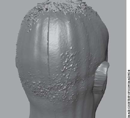
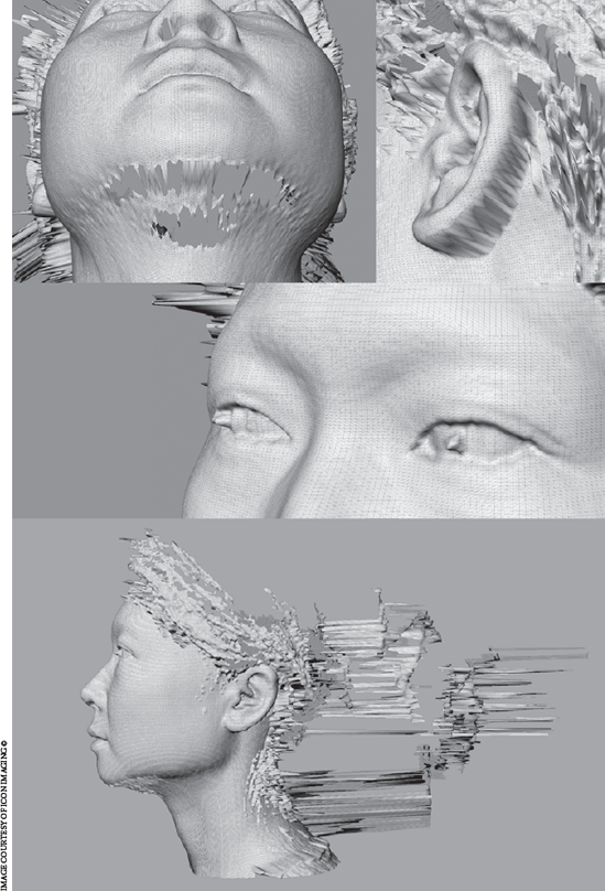
Figure 7.3. Scans showing a blind-area hole under the chin, anomalies on the ear, and reflective eye and hair
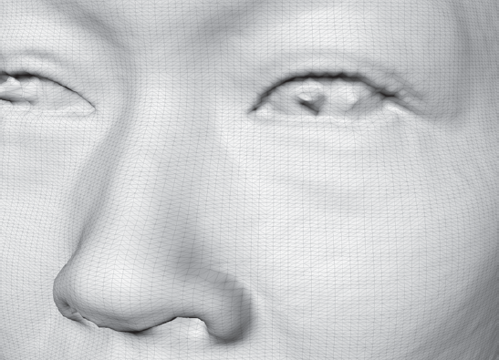
The solution to all these challenges is to start with a 3D scan of the subject, remove the anomalies from that scan, and transfer the likeness onto a polygonal topology that can be animated. This process is called 3D scan cleanup and re-topology. The 3D scan data is an excellent starting point to get the perfect likeness of a model. If you have modeled using image planes, think of the 3D scan data as a 3D image plane you can use as a reference to build the perfect model with the ideal topology. Starting with 3D scan data saves many hours of modeling work as it generates convincing likeness, accurate proportions, and comprehensive surface details (Figure 7.4).
Modelers and digital sculptors use the 3D scan data as a starting point and utilize the complex 3D scan mesh as a template to snap on their own points and polygons with the needed topology. This used to be a time-consuming process, but it is getting a lot less so, and much easier because of re-topology tools and plug-ins for major 3D modeling software.
Recently, with the introduction of digital sculpting tools such as Mudbox and ZBrush, this process has gotten even easier. Because digital sculpting software such as Mudbox enables the manipulation of multimillion-polygon models, modelers and digital sculptors can now easily use the sculpting tools to clean up the scan data, and then use a library of generic base mesh models onto which they wrap or project the 3D scan detail with relative ease and speedy results.
Three-dimensional scanners are machines that sample points on the surface of objects and create a set of 3D coordinates that represent these points. The density of these sampled points depends on the resolution of the scanners, and, of course, the denser the points, the more accurate the scan. Also, depending on your needs, some scanners also enable you to scan the same subject at different scan densities (Figure 7.5).
The information gathered by the 3D scanner is fed into 3D scan software that outputs the 3D scan mesh model. Because you can represent a plane by using three points in 3D space, the 3D scan software then algorithmically determines the optimal way to attach the scanned 3D coordinates into planes represented by triangles. The resulting mesh is a set of 3D coordinates and a list of which points are attached in triangles and then output in an exportable format such as an .obj file.
There are many types of 3D scanners, such as laser, structured-light, light detection and ranging (LIDAR), photometric, surface-transmitter, and touch-probe scanners. All of these scanners produce information that can be processed and refined in Mudbox. However, the two that are most commonly used are laser and structured-light 3D scanners.
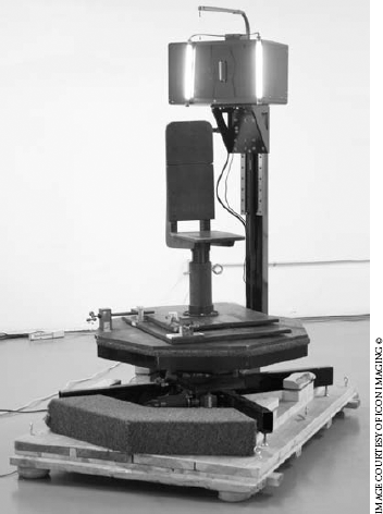
Laser scanners employ an array of lasers and cameras to record the coordinates of points on the surface of the scan subject (Figure 7.6). They are the most commonly used 3D scanners and are produced by companies such as Cyberware, Konica Minolta, and NextEngine.
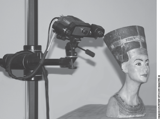
Structured-light scanners project patterns of parallel stripes that are observed by cameras at different viewpoints. These patterns on the surface of the scanned object appear geometrically distorted because of the surface shape of the object, and the cameras can triangulate the distortions into their locations in space. Structured-light scanners are produced by companies such as GOM International (ATOS scanners) and Steinbichler Optotechnik (Figure 7.7).
LIDAR measures the range of distant objects determined by calculating the time delay between the transmission of a laser pulse and a reading of the reflected signal. LIDAR is used mostly to scan points on distant large objects such as buildings.
Photometric scanners use silhouette, or photometric image data to generate the coordinates of the points on the surface.
Surface-transmitter scanners employ small transmitter objects that are placed on the surface of the object to transmit coordinates. These are used mostly for capturing motion, but they can also be used to get key defining coordinates of large objects.
Touch-probe scanners generate the 3D coordinates based on a sensor on a swiveling or robotic arm touching or colliding with the subject. Examples of these are 3D scanners produced by companies such as FARO Technologies and MicroScribe.
Three-dimensional scanning is still very much a developing technology with implementations in many scientific and commercial fields. Even though we have scanners that can capture perfect renditions of people and objects, advancements in research and development (R&D) labs are pushing the limits of precision, scale, speed of scanning, and ways of generating and manipulating the information.
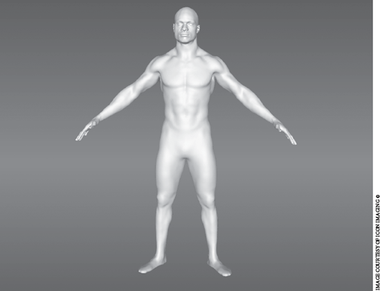
Theoretically, we are able to scan objects of any size, either by a single scan or by stitching together multiple scans. The most commonly scanned subjects are people's faces (Figure 7.8) or bodies (Figure 7.9), because they have unique identifying characteristics that are instantly recognizable, and yet are difficult and time-consuming to model, sculpt, and re-create.
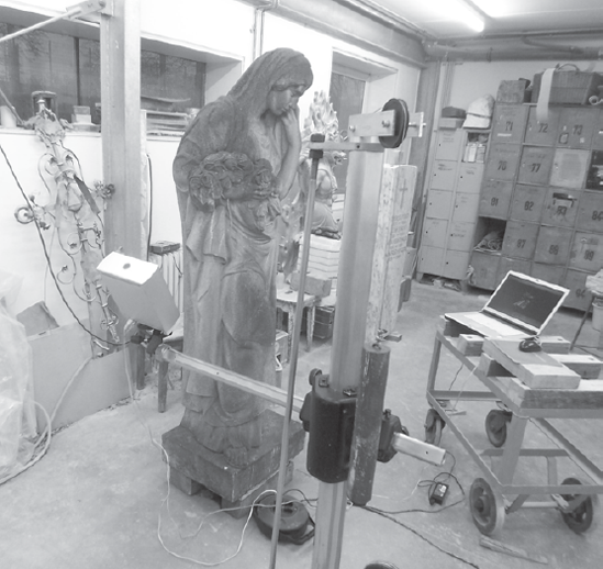
To accommodate for that, most commonly used 3D scanners are made to scan a face or a body. However, some scanners are made to scan larger objects, such as cars or statues (Figure 7.10), or smaller objects, such as a maquette (Figure 7.11) or action figure. Scanners can also scan multiple parts of an object and combine the scan pieces into one complete model.
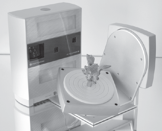
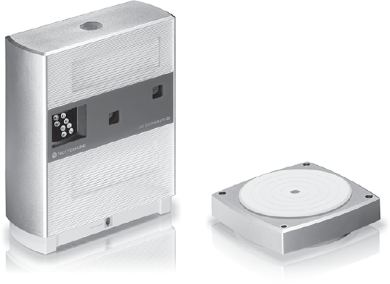
Most professional-grade 3D scanners are industrial-size devices used by professional 3D scanning companies. There are, however, smaller, less-expensive 3D scanners available that are the size of a cereal box, such as the NextEngine 3D scanner (Figure 7.12).
When you need scans of objects of varying sizes, you need to consider scan accuracy. Three-dimensional scan accuracy can range from meters for larger objects to millimeters and microns for smaller ones. Some scanners are able to sample points at the accuracy levels they publish, and others use algorithms to make approximations that fill in points between physical sample ranges. Of course, the data quality of the scanners that produce results based on sample points versus algorithmic approximation is more accurate, and less prone to softness in detail.
The data generated from 3D scans of heads or bodies are in the range of 500,000 to 1 million polygons (triangles). A maquette can be in the range of 1 to 10 million polygons. Some detailed car interior scans can go above the 50 million polygon range. There are detailed scans, such as the one done on Michelangelo's David, that exceed 1 billion polygons.
Most 3D scan data is collected and interpolated by scanning software that exports the results in formats readable by 3D and computer-aided design (CAD) applications. Most commonly, the file formats produced by 3D scanners are .obj, .ply (Polygon File Format), or .stl (Stereolithography). In Mudbox we will use the .obj format because it is the only one that's supported.
After you have the 3D scan data in .obj format, you load it into Mudbox to look at the results. As mentioned before, the polygon count you will be working with is in the 500,000 to 1,000,000 polygon range for a head or body, so Mudbox can easily handle that number of polygons. This would be a good way to visualize our model, and use the Rotate and Scale tools to arrange the model and orient it to the center of the screen.
One thing to make sure of is the direction of the normals. You need to make sure that the scan application exports the .obj file with normals facing outward. You get a visual cue of this in Mudbox as you load the model. If you get scan data with normals facing inward (Figure 7.13), you can either re-request the data with the normals facing outward or load the data into a 3D application and reverse the normals.
After you have the model loaded and positioned, you should visually check it for scan anomalies and take notes as to where they are, because you will have to fix them later.
Generally, 3D scanners have problems with the following surfaces:
Occluded areas that are blind spots for the scanner
Perfectly horizontal surfaces
Random spikes from floating particles in the air that may get caught in the scan
Reflective surfaces
Extremely dark or black surfaces that absorb light
Shiny surfaces that reflect light irregularly
Small multidirectional fibers such as hair
Surfaces with uniform textures or materials
Surfaces that have transparent or refractive properties
Some of these anomalies can be fixed before the scan. For example, to get a surface scan of a transparent, glass soda bottle, we would have to paint it with some opaque paint or add a layer of opaque powder. To get rid of anomalies caused by hair, we would have the model wear a skull cap. To get rid of anomalies caused by reflective surfaces, we would coat the surface with a nonreflective substance. Other anomalies can be fixed after the scan by sculpting the corrections.
In the rest of this chapter, you will go through the process of bringing 3D scan data into Mudbox and mapping the detail onto a more manageable topology. If you will not use 3D scan data, this process is also critical to the Mudbox workflow because you would use this exact same process to re-topologize a sculpture you created from scratch that needs to be mapped onto a more manageable topology. Let's say, for example, you sculpted a creature's head by using the Sphere primitive. It started out as a sketch, but you got some amazing results and wanted to get better topology to continue to add more detail or to send the model off to be animated. The process used to apply your sculpt onto a more accommodating topology mesh would be the same method we will be going through to re-topologize a 3D scan.
In the rest of this chapter, you will load a 3D head scan and go through the following steps to apply a new topology to it:
Load the 3D scan data into Mudbox.
Edit some of the anomalies in an external 3D application.
Add the Mudbox Basic Head primitive to the scene and align it to the 3D scan.
Extract a displacement map.
Apply the displacement map back on the model by using the Sculpt Model Using Displacement Map function.
Sculpt out the anomalies and add sculptural details.
Let's get started.
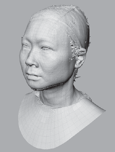
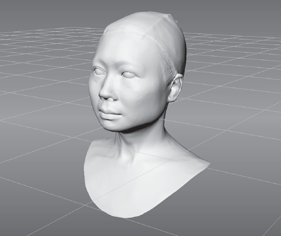
The 3D scan data you will work with in this chapter is provided by Icon Imaging, one of the leading studios that specializes in very realistic and complex 3D scanning, modeling, and imaging (I have included information about Icon Imaging in the acknowledgments section at the beginning of this book). The scan artists at the company used a Cyberware 3D head scanner, which orbits 360 degrees around a subject's head, to produce the scan data. Typically, 3D scan houses offer various levels of data cleanup services, but I asked for this data in its rawest form to give you an idea of the anomalies that happen during a typical scan. The resulting scan (Figure 7.14) has some excellent examples of anomalies.
Start Mudbox. Choose File → Import and import the
Chapter 7
aw_head_scan.obj
file from the DVD. Click OK to close the warning dialog box. This warning dialog box will always come up if you are importing a high-resolution mesh with no subdivision levels. It will take from a few seconds to a few minutes, based on your system, to load the 3D scan mesh. Choose the white Chalk or Gesso material from the Material Presets tray. In the Object List, note that the 3D scan has 374,408 polygons.Zoom in on the scanned head. Notice that as you get "closer" to the head, and it starts getting bigger, a big hole appears in the model (Figure 7.15).
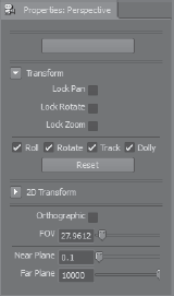
This happens because the model is intersecting your near plane. The near plane is also referred to as the near clipping plane, and it defines how close the camera sees. The reason that the model is cutting out is because the default near plane value of 1 does not give you enough room to see the entire image. You can remedy this situation by selecting the Perspective camera in the Object List tray, and setting the Near Plane attribute to 0.1 (Figure 7.16). If you are not able to see the model, remember to press the A key on your keyboard to center the model in the viewport.
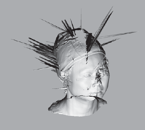
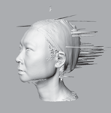
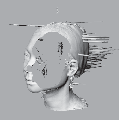
Tumble around the model and look at the captured detail of the face in addition to all the anomalies. The most obvious ones are the porcupinelike spikes and the holes at the top and the bottom of the chin and the cap. You will also see some little spikes from the hair, between the top of the hair and the cap, and the reflective eyeballs. There is a little anomaly on the top of the head from the calibration pendulum of the scanner. Notice the subtle ripples on the face from the scan. This is most noticeable below the right eye and the neck area. Notice that there is a sharp drop-off behind the ear, where there is an occluded area. Finally, even though this scan was completed in under a minute, note the ridge line in the back, indicating where the scan started and ended (Figure 7.17). This is considered a good scan of someone who is very experienced at being scanned, and as you can see, there still are some unavoidable anomalies.
Choose Create → Mesh → Basic Head to add the Mudbox Basic Head primitive to the scene. You might be surprised, because you will not see anything happen. That's because the Basic Head scale is significantly bigger than the scanned head image. Press the A key, and you will see the Basic Head primitive but not the scanned head. As you tumble around in your scene, you will notice that the 3D scanned head is tiny compared to the Basic Head primitive. This is another big anomaly to take into consideration: the scale of the 3D scan.
Even though it is possible to clean up all of the anomalies in Mudbox, I find it easier to do some of the cleanup in another 3D application that gives me more control over deleting polygons. In either Maya 2010 or Softimage 2010, you can easily import the 3D scan data and delete the polygons that make up the spikes. It is a process that takes very little time because you can bulk-select the spike pivot points and the polygons they contain, and then delete them. I also deleted the pendulum geometry above the head because it was not needed.
The next thing I did was export the Basic Head primitive from Mudbox as an .obj file and import it into Softimage 2010. I translated, rotated, and scaled the 3D head scan to approximately match the same size, orientation, and centered position as the Basic Head Mudbox primitive. I exported the edited 3D head scan from Softimage 2010 as head_scan_Softimage_edit.obj for you to use for this chapter.
The 3D scanning companies that you get your 3D scan from will, in most cases, do this cleanup for you, but it's also good to know how to do the edits yourself just in case you need to. Here are the steps:
Choose File → New Scene without saving your prior work. Then choose File → Import and import the
Chapter 7head_scan_Softimage_edit.objfile from the DVD. Again, click OK to close the warning dialog box that comes up. Choose the white Chalk or Gesso material from the Material Presets tray. Notice that the bigger spikes are gone, but all the other anomalies are still there.Press the W key on your keyboard to bring up the wireframe on the face (Figure 7.18).
You can now see why this model, while instantly recognizable as the scanned person, is completely not feasible to sculpt, patch up, or animate. Select the face by clicking the Objects tool in the Select/Move Tools tray. Click the UV View tab in the main viewport. Notice that the 3D scan does not have any UVs, nor would you want to UV a model this messy. Click back on the 3D view and press the W key to turn off the wireframe.
What you need to do is take the best of what the 3D scan has to offer and apply it to a more manageable mesh. In this case, you will use the Basic Head primitive from Mudbox. You could use one of the many human head base meshes that are available on the Internet for free or, of course, one of your own. As you already know, the Basic Head base mesh in Mudbox has UVs and has a topology you can subdivide and sculpt.
Choose Create → Mesh → Basic Head. This adds the Basic Head primitive to your scene. Notice that there is a little overlap of both the meshes. Select the Basic Head and subdivide it one level by pressing Shift+D.
In the Object List, click the padlock icon next to the
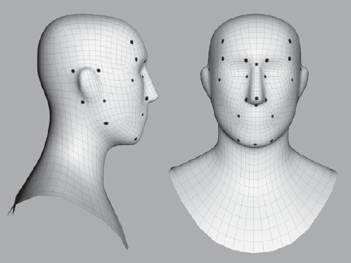
head_scan_Softimage_edit_0object to lock it. You need to do this because you want to make sure you don't move any of the points on the scanned 3D head.Select the Grab tool from the Sculpt Tools tray. Using appropriate Size and Strength, align key landmarks (Figure 7.19) of the Basic Head primitive to those of the 3D scanned head. Press the W key to turn on the wireframe and make sure that your quads are well spaced and not overlapping or squashed together. Your alignment does not have to be precise, but the landmarks should roughly overlap those on the 3D scan.
By the time you are finished, your head should look more or less like Figure 7.20. You can import
Mudbox_basic head_edit.objfrom the DVD to check your work.
In this section, you will be extracting the displacement map of the 3D scanned head—but with a twist. You will use the 3D scanned head as the source model and the Basic Head primitive as the target model during your extraction. This will extract the displacement, or surface depth information, of the high-resolution mesh and map it onto the UVs of the Basic Head.
Choose Maps → Extract Texture Maps → New Operation.
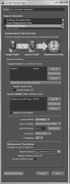
Select the Displacement Map check box to expand the dialog box and bring up the options for extracting a displacement map. All the settings that we will discuss can be seen in Figure 7.21.
Next to the Target Models (Low Resolution Mesh) list box, click the Add All button. This adds both the 3D head scan and the edited Basic Head primitive to the list. Click the 3D scan data head (
head_scan_Softimage_edit_0) and click the Remove button.Do the same for the Source Models (High Resolution Mesh) list box but remove the Basic Head primitive (
Head_0) from the list.Make sure Locate Method is set to Raycasting, and for the Search Distance option, click the Best Guess button. This sets the total distance that samples can be taken from the target model to the source model based on the distances between the bounding boxes of the two.
In the Choose Samples list, make sure Closest to Target Model is selected. This creates the displacement map with samples closest to the target model.
Select an Image Size of 4096 × 4096, because you want to use the maximum map size to get the most detail from the 3D scanned model.
Click the folder icon next to the Base File Name text box and type
3Dscan_displacementor a name of your choice for your displacement map. Select OpenEXR [32 Bit Floating Point, RGBA] as the file format and click Save. Again, this does not generate or save the displacement map; it just sets the name.Make sure the Preview as Bump Layer option is not selected.
Click the Extract button to extract the displacement map. This opens the Map Extraction Results dialog box, which shows you the progress of the extraction.
The dialog box tells you that your map extraction finished without errors and the operation completed successfully. Click OK, and click Close to close the Map Extraction Results dialog box.
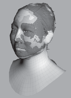
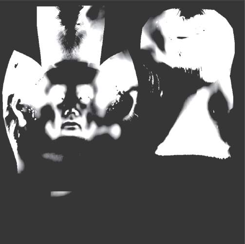
Click the Image Browser tab in the main viewport and navigate to the folder in which you extracted the displacement map. Examine the displacement map (Figure 7.22). You can use the + or – keys to increase or decrease the stop value, respectively, to see the level of detail the image has at different exposures. Also note that the displacement map has been extracted to match the UV map of the Mudbox Basic Head primitive.
At this juncture, you no longer need the 3D scan model. You will delete it and wrap the displacement map you generated to add the details of the 3D scan to a subdivided version of the Mudbox Basic Head primitive.
Select the 3D head scan (
head_scan_Softimage_edit_0) in the Object List tray, right-click on it, and select Delete Object. This leaves the Mudbox Basic Head primitive you edited earlier. Select the head (Head_0) in the Object List and press Shift+D four times to get about 512,000 polygon subdivisions. We can further subdivide our model, but a good guideline is to get as close to the same number of polygons as the 3D scan model, which is 374,408.Choose Maps → Sculpt Model Using Displacement Map → New Operation.
From the Target Mesh list box, select the only mesh in the scene:
Head_0.Click the three dots next to the Displacement Map text box, select the displacement map you generated in the previous section (
3Dscan_displacement.exr), and click Open.Click Go. This displaces your Basic Head primitive.
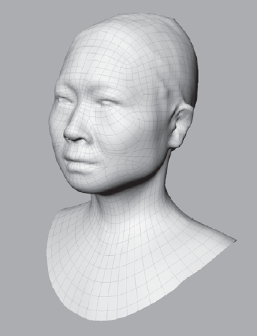
Note that you now have the exact same model of the 3D scan, but if you press the W key, you will see that it is no longer composed of triangles and n-gons but of quads that the Basic Head primitive was composed of (Figure 7.23). You have solved one of the big problems you had.
Tumble around the head and notice that the holes have been filled, and that's another problem solved. But the model has a lot of little spikes, surface inconsistencies where the holes used to be, anomalies behind the ears, and so forth, that still need to be fixed.
You can no longer solve any of the remaining anomalies automatically. You will need to use good old digital sculpting to get the model to look like the scanned subject. Fortunately, this is not too difficult and is perfectly suited for Mudbox. To sculpt out the anomalies, it is easier to start at the lower subdivision levels and work your way up.
You will initially use three sculpt tools—the Smooth, Grab, and Flatten tools—and then use the Sculpt and Wax tools to sculpt some details. Always remember, it is a good idea to use sculpt layers and to save often. It is also a good idea to use lower Size and Strength settings and work your way up.
Press Pg Dn until you are at level 1. Use the Grab and Smooth tools to move the polygons in the neckline area so they align. Use the Smooth tool to straighten some of the artifacts that can be seen at this level. Remember to use an additive approach to smoothing by using a lower Strength setting, testing it out, and then gradually working your way up to a greater Strength or applying the Smooth tool with the weaker Strength a few times to get the desired effect. Use the Grab tool to gradually lift up the top of the head where the hole used to be. By the end of your work, your sculpture should look like Figure 7.24.
Step up one level to level 2 by pressing Pg Up. Repeat the process in step 1 to sculpt out the anomalies that show up. Note that there are still anomalies in the areas you fixed on level 1, but they are less severe than they would have been had you not done the work on level 1.
Step up to level 3 by pressing Pg Up. Now you can see some of the anomalies in more-granular detail. At this level, as you are getting rid of anomalies, you could just as easily also soften up needed surface details. So, from this point on, it is a good idea to use a lighter hand on the tablet and really work with smaller tool sizes and a lower Strength setting. Start out with the Smooth tool and move the tool in a circular motion over the anomalies to reduce their size. If the spikes persist, try using the Flatten tool, or drop back down a subdivision level and work on the same area.
Note
You might be tempted to press Shift to switch to the Smooth tool. However, this might prove problematic if you have the Smooth tool's Remember Size property selected. Pressing the Shift key will then revert to your last set Smooth tool and Size. I recommend that you do not have this option selected so that your smoothing size and strength match those of the tool you are using before you press the Shift key.
Step up to level 4 by pressing Pg Up. You can now see the anomalies in even more granular detail. Repeat the same work to smooth the anomalies. If you get into severe areas that need repair—for example, the neckline (Figure 7.25)—you can use the Flatten tool in combination with the Smooth tool to straighten up that area.
Press Shift+D to add another subdivision level, level 5.
Work with even more detail and fix the rest of the anomalies. Don't worry about losing some high-frequency detail such as skin pores or wrinkles, because those can easily be added at a later point. You might also lose some detail in areas critical to the sculpture, for example, some wrinkles on the cap or inside or around the ear, but those are easy enough to sculpt after you are finished with the cleanup.
At this point, the cleanup is done. Now is the time to sculpt the missing details, such as the inside of the ears, the indentation behind the ears, the nostrils, and all the other areas that you feel need detail.
I have included the version I worked on, named 3DScan_cleanup_final.mud, on the DVD in the Chapter 7 folder (Figure 7.26). I also included a couple of Sphere primitives, eye_lf.obj and eye_rt.obj, that you can use for the eyeballs. To add the eyeballs, import the two .obj files and use the Translate tool from the Select/Move Tools tray to position them. After they are positioned, you might want to sculpt the slight bulge of the cornea. I did not do any high-frequency detail on my version. In fact, I removed all the high-frequency detail because I was shooting for a more statuesque result, but you might want to add detail to your heart's desire. I have also included a video, Chapter7-working_with_3D_scan_data.mov, of my going through the entire process in the Chapter 7Videos folder.
When you are finished, you have a model with a believable likeness of the 3D scan subject, with UVs and usable topology that you can 3D-paint, further sculpt, or move into the next stages of the pipeline to get animated or 3D printed.
Three-dimensional scanning is an efficient method for getting near-perfect likenesses in little time, with very little specialized effort, and for nominal cost by using tools such as Mudbox.
The displacement map generation and the Sculpt Model Using Displacement Map technology in Mudbox, paired with the digital sculpting tools, have proven a great asset to many production pipelines.