Chapter 3

Parallel Studio XE for the Impatient

What's in This Chapter?

An overview of the four-step methodology for adding parallelism

Using Cilk Plus to add parallelism

Using OpenMP to add parallelism

The previous chapter introduced three ways of using Intel Parallel Studio XE: Advisor-driven design, compiler-centric development, and a four-step methodology.

This chapter describes the four-step methodology for transforming a serial program into a parallel program. The chapter's hands-on content guides you through the steps to create a completely parallelized program.

In the examples in this chapter, you use two parallel models, Intel Cilk Plus and OpenMP, to add parallelism to the serial code. Cilk Plus is regarded as one of the easiest ways to add parallelism to a program. OpenMP is a well-established standard that many parallel programmers have traditionally used.

You use various key components of Intel Parallel Studio XE to achieve the parallelization. This chapter describes how to use Intel VTune Amplifier XE 2011, an easy-to-use yet powerful profiling tool, to identify hotspots in the serial application, as well as analyze the parallel program for synchronicity, efficiency, and load balancing.

You use Composer XE to build the newly parallelized application, and then use Intel Inspector XE 2011 to reveal threading and memory errors. Finally, you return to Amplifier XE to check for thread concurrency and fine-tuning.

The Four-Step Methodology

Initially, parallelizing a serial program may seem fairly simple, with the user following a set of simple rules and applying common sense. But this may not always achieve the most efficient parallel program running at the expected speeds. Indeed, it is possible that faulty attempts at parallelization will actually make a program run more slowly than the original serial version, even though all parallel cores are running.

The four-step methodology, as shown in Figure 3.1, is a tried and tested method of adding parallelism to a program.

Figure 3.1 The four-step methodology

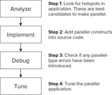
With the exception of the debug step, you should carry out the steps on an optimized version of the application.

Example 1: Working with Cilk Plus

In this example, you add parallelism to a serial program using Cilk Plus. Later, you parallelize the same serial code using OpenMP.

Obtaining a Suitable Serial Program

Not all serial programs are suitable for making parallel. Parallelization itself carries an overhead, which you must take into account when considering whether a program would benefit from being parallelized. You must test parallel programs extensively both by running them and by using analytical tools to ensure their results are the same as their serial versions.

Listing 3.1 shows the simple serial program that you'll make parallel using the four-step methodology. This is a contrived program, put together to show parallelization problems.

The program incorporates two loops: an outer loop and an inner work loop. The outer loop is designed to run the timed inner work loop several times; this reveals variations in timings caused by other background tasks being carried out by the computer. The time taken for the work loop to run is captured and reported back. The work loop itself iterates many times, with each iteration containing two further nested loops that calculate the sums of arithmetic series. The number of terms in the two series is determined by the loop count of the work loop. That is, as the work loop iteration count increases, the number of terms in the series increases, meaning that more work is required to calculate each series.

Then the inverse of the square root of each series is added to a running total; this is output at the end of the work loop. This stops the compiler from optimizing all the calculated values out of existence. Also, the output after each work loop has finished reveals the number of times the work loop has iterated, and the time taken for it to run.

Listing 3.1: The starting serial program

// Example Chapter 3 Serial Program
#include <stdio.h>
#include <windows.h>
#include <mmsystem.h>
#include <math.h>

const long int VERYBIG = 100000;

// ***********************************************************************

int main( void )
{
  int i;
  long int j, k, sum;
  double sumx, sumy, total;
  DWORD starttime, elapsedtime;

// -----------------------------------------------------------------------

  // Output a start message
  printf( "None Parallel Timings for %d iterations

", VERYBIG );
    
  // repeat experiment several times
  for( i=0; i<6; i++ )
  {
    // get starting time
    starttime = timeGetTime();

    // reset check sum & running total
    sum = 0;
    total = 0.0;
    // Work Loop, do some work by looping VERYBIG times
    for( j=0; j<VERYBIG; j++ )
    {
      // increment check sum
      sum += 1;

      // Calculate first arithmetic series
      sumx = 0.0;
      for( k=0; k<j; k++ )
        sumx = sumx + (double)k;

      // Calculate second arithmetic series
      sumy = 0.0;
      for( k=j; k>0; k-- )
        sumy = sumy + (double)k;

      if( sumx > 0.0 )total = total + 1.0 / sqrt( sumx );
      if( sumy > 0.0 )total = total + 1.0 / sqrt( sumy );
    }

    // get ending time and use it to determine elapsed time
    elapsedtime = timeGetTime() - starttime;

    // report elapsed time
    printf("Time Elapsed %10d mSecs  Total=%lf   Check Sum = %ld
",
                  (int)elapsedtime, total, sum );
  }

  // return integer as required by function header
  return 0;
}

// **********************************************************************

code snippet Chapter33-1.cpp

Even novice C programmers should have no problem understanding most of this program; however, it does contain a few lines of code that merit explanation. The program uses calls to the Windows API function timeGetTime(), which returns the current system time in milliseconds. By calling this function before and after the main work loop, you can determine the time involved in executing the loop. The time is returned by the function in a DWORD type variable. Looking at the start of the program code, you can see that a number of declarations are made:

• #include <stdio.h>, to enable input and output to and from the program in the usual manner.
• #include <windows.h>, to enable DWORD variable types to be declared.
• #include <mmsystem.h>, because it holds the prototype of the library function timeGetTime().
• const long int VERYBIG 100000, which sets a constant that is used to control the number of times the main work loop will repeat. This is the controlling variable, which you can alter to vary the amount of work to be carried out, and therefore the length of time taken. This is shown as 100000.

Running the Serial Example Program

Before you undertake any parallelism, it is a good idea to build and run the existing serial version of the program. This gives a benchmark for the application and also shows what the output should look like. After parallelization, you should always check that the output of the program remains the same as for the serial version.

Creating the Project

To create a new project in Microsoft Visual Studio, perform the following steps:

Figure 3.2 Selecting the Release configuration

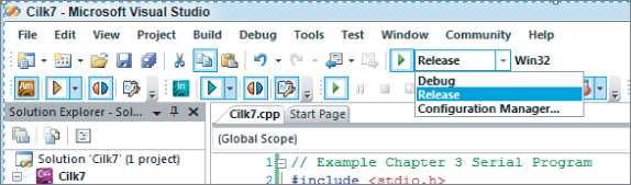
Figure 3.3 Adding winmm.lib to the linker options

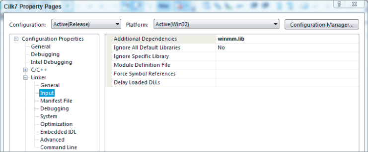
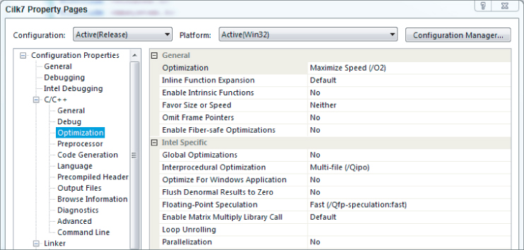
Figure 3.4 Optimizing for speed

Running the Serial Version of the Code

You will be building two serial versions of the application; the first version uses the Microsoft compiler, and then the second version uses the Intel compiler.

Using the Microsoft Compiler

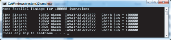
You are now ready to build and run the serial example. The example program can be built using the Microsoft compiler in the usual manner. You can launch the program from within Visual Studio by pressing Ctrl+F5. Figure 3.5 shows the output, using the initial controlling constant VERYBIG set as 100000. Your output timings may be different due to differences between computer systems.

Figure 3.5 Serial timings for 100,000 iterations using the Microsoft compiler

Using the Intel Compiler

The first version of the program was built using the Microsoft compiler. To change to use the Intel compiler, follow these steps within the Microsoft Visual Studio environment:

You should find that the executable runs a lot faster, as shown in Figure 3.6. This is because the Intel compiler optimizer is smarter about removing and refactoring redundant or expensive computations.

Figure 3.6 Serial timings for 100,000 iterations built with Intel compiler

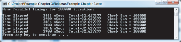
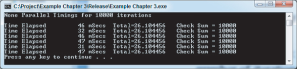
The check sum value is a consistent 100000, which is the same as the number of iterations of the inner or working loop. The Total value is the result of the arithmetic calculations involved within the inner loop. If you want to reduce the time taken to run the program, make the value of VERYBIG smaller. Figure 3.7 shows the output run for a value of 10000.

Figure 3.7 Serial timings for 10,000 iterations

Step 1: Analyze the Serial Program

The purpose of this step is to find the best place to add parallelism to the program. In simple programs you should be able to spot obvious places where parallelization might be applied. However, for any program of even just moderate complexity, it is essential that you use an analysis tool, such as Intel Parallel Amplifier XE. Although this is a rather trivial programming example, you can use the steps on more complex programs.

Using Intel Parallel Amplifier XE for Hotspot Analysis

When Intel Parallel Studio XE was installed into Microsoft Visual Studio, it set up a number of additional toolbars, one of which is for Intel Parallel Amplifier XE (introduced in Chapter 2). Amplifier is a profiling tool that collects and analyzes data as the program runs.

This example uses Amplifier XE to look for parts of the code that are using the most CPU time; referred to as hotspots, they are prime candidates for parallelization.

Because Amplifier XE does slow down the execution of the program considerably, it is recommended that you run an application with reduced data. Provide data input and reduce loop iterations, where possible, to reduce the run time.

For this example, the outer loop is reduced to 1. This will not prevent Amplifier from finding the hotspots, because the outer loop merely runs through the same work loop several times. Hotspots found in the first iteration of the work loop will be the same in any further iterations of it. Also, leave VERYBIG set as 10000. You will need to rebuild with these new settings before using Amplifier.

Starting the Analysis

To start the analysis, follow these steps:

Figure 3.8 Selecting a new Amplifier analysis

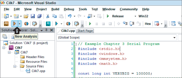
Figure 3.9 Start-up page of the Amplifier XE

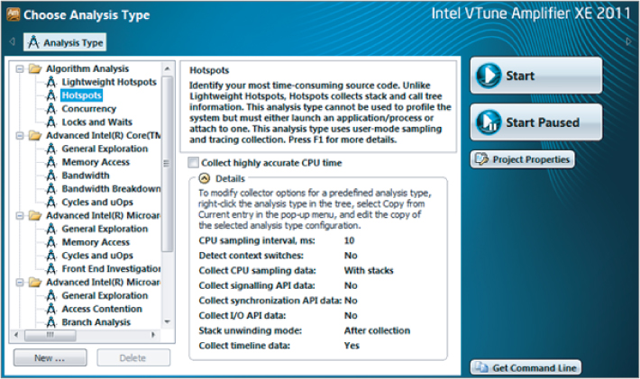
Figure 3.10 shows the results.

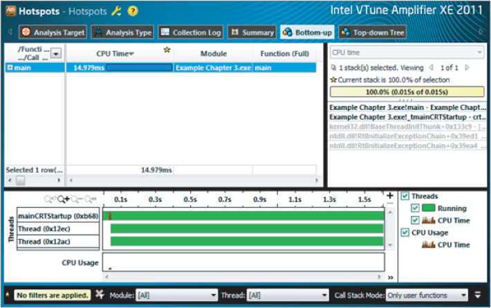
Figure 3.10 Hotspot analysis using Amplifier XE

Drilling Down into the Source Code

Figure 3.10 shows how much CPU time was spent in each function. In this example, because there is only a single function, main, only this one entry is present. To examine the source code of the hotspot, double-click the entry for function main. This reveals the program code, with the hotspots shown as bars to their right with lengths proportional to CPU time spent on each line (Figure 3.11). Note that the code pane has been expanded within the Amplifier window, and that line numbers within Parallel Studio have been turned on.

Figure 3.11 Hotspot analysis using Amplifier XE, showing hotspots

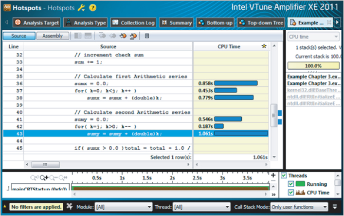
In the code shown, Amplifier automatically centers on the line of code that consumes the most CPU time — in this case, line 43. Two groups of three lines are using most of the CPU time; these involve the loops calculating the two arithmetic series. The remaining code lines consume little CPU time in comparison and so show nothing. These arithmetic loops are the hotspots within your program. Your own computer system may give different times, but it should follow a similar pattern.

You should also note that the Amplifier results for this run are placed in the Amplifier XE folder under the project solution. You can see this to the left of the screen.

Parallelization aims to place hotspots within a parallel region. You could just attempt a parallelism of each of the arithmetic loops. However, parallelization works best if the largest amount of code can be within a parallel region. Parallelizing the work loop places both sets of hotspots within the same loop.

Step 2: Implement Parallelism using Cilk Plus

After identifying the hotspots in the code, your next step is to parallelize the code in such a way as to include the hotspots within a parallel region.

To make the code parallel, follow these steps:

#include <cilk/cilk.h>

// Work Loop, do some work by looping VERYBIG times
cilk_for( int j=0; j<VERYBIG; j++ )

// Output a start message
printf( "Cilk Plus Parallel Timings for %d iterations 

",VERYBIG );

And that's it! Simple, isn't it?

Well, not quite. You have a few problems to overcome. You should rebuild a Release version of your program with VERYBIG set as 10000, but change your outer loop count back to the original 6.

When your program now runs, it creates a pool of threads, where the number of threads is usually the same as the number of cores. These threads are made ready to be available within the parallel regions. When a parallel region is reached, such as the cilk_for loop, the threads distribute the work of executing the loop among themselves dynamically. This should, in theory, speed up the execution time.

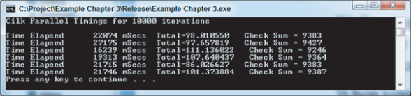
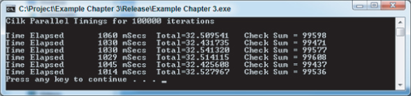
In fact, when you now run your program, you will find that instead of reducing the execution time, it has actually increased it enormously. Figure 3.12 shows the new timings, using a 4-core installation. Compare these timings with the serial version shown in Figure 3.7; the parallelized version is much slower. And remember that all 4 cores were running, so it is actually four times slower than the numbers suggest. Also, notice the values of Total and Check Sum are incorrect.

Figure 3.12 Timings for the initial Cilk Plus parallelized program

Obviously, something is wrong. The problem is, by introducing parallelism, you also introduced problems caused by concurrent execution. In the next few steps you investigate how to fix these problems by enhancing both the speed and performance of the application.

Step 3: Debug and Check for Errors

With the introduction of parallelism into the program, the program no longer runs correctly. This step checks the program to see if any parallel-type errors exist, such as deadlocks and data races, which are responsible for slowing down the program. These errors are caused by multiple threads reading and writing the same data variables simultaneously — always a potential cause of trouble.

Checking for Errors

You can find data races and deadlocks by using Intel Parallel Inspector XE. It is recommended that you perform any error checking on the debug version of the program, not the Release version. Building in the Release version will carry out optimizations, including in-lining, which may accidentally hide an error. Using the debug build also means that the information reported by Inspector is more precise and more aligned with the actual code written.

Running an Inspector analysis is a lot slower than just running the program normally. As with Amplifier, you should reduce the running time by reducing loop counts and using small data sets.

To check for errors, follow these steps:

// repeat experiment several times
for( i=0; i<1; i++ )

Figure 3.13 Selecting a new Inspector analysis

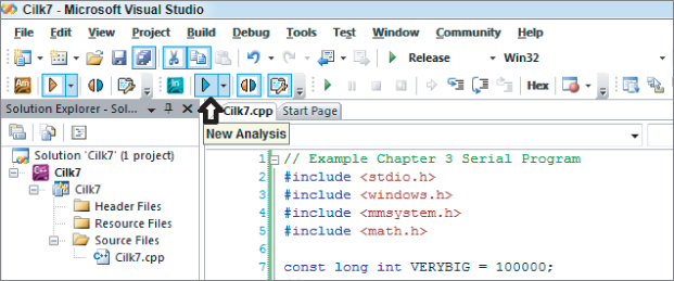
Figure 3.14 Selecting for locating deadlocks and data races

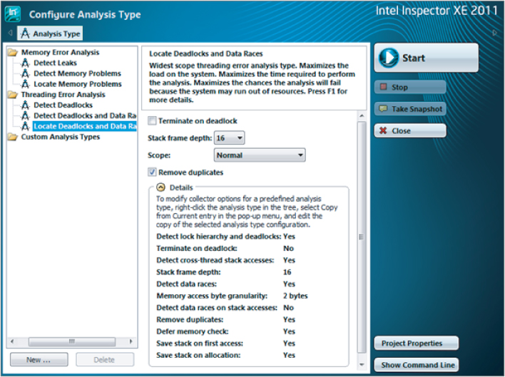
Figure 3.15 Summary of threading errors detected by the Inspector XE analysis

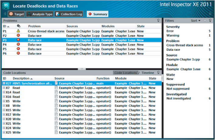
Figure 3.16 A data race exposed in the source code

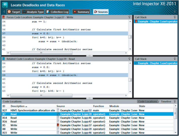
From these two code snippets you can determine that variable sumx is the problem. The Focus Code Location pane shows the variable being changed (write), at line 37 of the code. The Related Code Location pane shows the variable being read, at line 39 of the code. When multiple threads are running there arises the danger of one thread changing the value of sumx (resetting to 0), while a second concurrently running thread is still using it, thereby making the second thread have an incorrect value. This is referred to as a data race.

Examining the other data race problems, you should be able to determine which variables they involve. The full list of variables causing data races is sum, total, sumx, sumy, and k. All five of these variables were created at the start of the function, and their scope is that of the function. However, the arguments that follow would be the same regardless of whether these variables are global or static. During parallel execution all the threads are competing to read from and write to these function-scoped variables. These are referred to as shared variables, and they are all shared by the concurrently executing threads. For future reference, they will be referred to as nonlocal variables.

Narrowing the Scope of the Shared Variables

Looking at the variables k, sumx, and sumy, you can see that they are set and used wholly within the parallel region; they are not used outside it. One solution for this is to declare them within the parallel region. As each thread independently runs through the code of the parallel region, it creates its own private versions of these variables. They will be local variables to each thread.

Indeed, this is exactly what happened when the Cilk Plus version of the for loop was declared: its loop variable j was declared within the loop control bracket. It is a local variable that will be private for each thread.

You can modify the first few lines of the work loop, as shown in Listing 3.2. You can remove the original declarations of these variables from the top of the program if you wish. Removing them cleans up the program and makes it easier for other programmers to understand; however, if you don't remove the variables from the top of the program, the compiler simply creates locally scoped variables that overlay the variables at the top of the program. This also applies to loop counter j, which was redeclared within the loop control bracket.

Listing 3.2: Amendments to beginning of the work loop for Cilk Plus implementation

// Work loop, do some work by looping VERYBIG times
cilk_for( int j=0; j<VERYBIG; j++ )
{
  long int k;
  double sumx, sumy;

  // increment check sum
  sum += 1;

code snippet Chapter33-2.cpp

Set the work loop controlling variable VERYBIG to 100000, and the outer loop iteration value back to 6. Then rebuild a Release version of the application and rerun. Figure 3.17 shows the timings for this new run on a 4-core machine. Remember, your actual values may be different for your computer.

Figure 3.17 Timings for the Cilk Plus parallelized program using loop local variables

Notice that the Total and Check Sum values are incorrect and inconsistent between the runs. These errors are also caused by data races, but making thread-private copies of the offending variables total and sum locally within the loop will not help in this case, because these variables must be shared between all the threads.

Figure 3.18 illustrates what happens when more than one thread attempts to increment the check sum in the code line:

sum += 1;

Figure 3.18 Problematic access to global variables

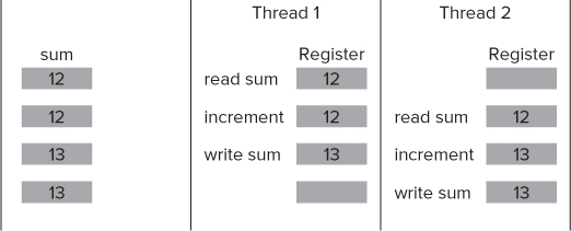
As you can see from Figure 3.18, if sum starts with a value of 12, after both threads have incremented the result is 13, instead of the expected 14.

One solution for a variable of this type is to use a synchronization object or primitive, such as a lock. This ensures that only a single thread at a time has access to it. Other threads requiring access at the same time must wait for the variable to become free. However, this solution has the drawback of slowing down the execution time. Alternatively, Cilk Plus offers a special variable form called a reduction variable, which is discussed in the next section.

Adding Cilk Plus Reducers

Cilk Plus reducers are objects that address the need to use shared variables in parallel code. Conceptually, a reducer can be considered to be a shared variable. However, during run time each thread has access to its own private copy, or view, of the variable, and works on this copy only. As the parallel strands finish, the results of their views of the variable are combined asynchronously into the single shared variable. This eliminates the possibility of data races without requiring time-consuming locks.

A Cilk Plus reducer is defined in place of the normal nonlocal shared variable definition. Remember that here, nonlocal refers to automatic and static function variables as well as program global variables. The Cilk Plus reducer has to be defined outside the scope of the parallel section of code in which it is to be used.

To add Cilk Plus reducers to the code, follow these steps:

   #include <cilk/reducer_opadd.h>

 cilk::reducer_opadd<long int> sum(0);
 cilk::reducer_opadd<double> total(0.0);

 sum = 0;
 total = 0.0;

 printf("Time Elapsed %10d mSecs  Total=%lf   Check Sum = %ld
",
        (int)elapsedtime, total.get_value(), sum.get_value() );

Listing 3.3 gives the final Cilk Plus program.

Listing 3.3: The final version of the Cilk Plus parallelized program

// Example Chapter 3 Cilk Plus Program
#include <stdio.h>
#include <windows.h>
#include <mmsystem.h>
#include <math.h>
#include <cilk/cilk.h>
#include <cilk/reducer_opadd.h>

const long int VERYBIG = 100000;

// ***********************************************************************

int main( void )
{
  int i;
  DWORD starttime, elapsedtime;

// -----------------------------------------------------------------------

  // Output a start message
  printf( "Cilk Plus Parallel Timings 

" );
    
  // repeat experiment several times
  for( i=0; i<6; i++ )
  {
    // get starting time
    starttime = timeGetTime();

    // define check sum and total as reduction variables
    cilk::reducer_opadd<long int> sum(0);
    cilk::reducer_opadd<double> total(0.0);

    // Work Loop, do some work by looping VERYBIG times
    cilk_for( int j=0; j<VERYBIG; j++ )
    {
      // define loop local variables
      long int k;
      double sumx, sumy;

      // increment check sum
      sum += 1;

      sumx = 0.0;
      for( k=0; k<j; k++ )
        sumx = sumx + (double)k;

      sumy = 0.0;
      for( k=j; k>0; k-- )
        sumy = sumy + (double)k;

      if( sumx > 0.0 )total = total + 1.0 / sqrt( sumx );
      if( sumy > 0.0 )total = total + 1.0 / sqrt( sumy );
    }

    // get ending time and use it to determine elapsed time
    elapsedtime = timeGetTime() - starttime;

    // report elapsed time
    printf("Time Elapsed %10d mSecs  Total=%lf   Check Sum = %ld
",
          (int)elapsedtime, total.get_value(), sum.get_value() );
  }

  // return integer as required by function header
  return 0;
}

// **********************************************************************

code snippet Chapter33-3.cpp

Running the Corrected Application

Figure 3.19 shows the application's new timings on a 4-core machine after you have fixed all the errors and rebuilt a new Release version. Again, these timings were generated on a 4-core computer system and may differ from your timings, depending on what system you are running.

Figure 3.19 Timings for the Cilk Plus parallelized program with reducers added

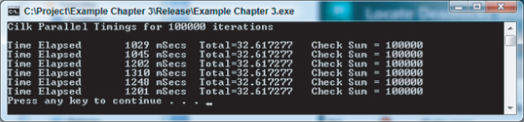
A speedup ratio of about 3.74 was achieved compared to the speeds shown in Figure 3.6. The Check Sum and Total values are now correct, being the same as in the serial version of the program. Running the Intel Parallel Inspector again shows that the data race problems have been resolved.

It is important to note that using the Intel C++ compiler with Cilk Plus parallelization has sped up the process approximately 13 times over the timings obtained using the default Microsoft C++ compiler shown in Figure 3.5.

Step 4: Tune the Cilk Plus Program

Cilk Plus works by allowing the various parallel threads to distribute work among themselves dynamically. In most cases this leads to a well-balanced solution; that is, each thread is doing an equal amount of work overall. To use Intel Parallel Amplifier XE to check for this concurrency and efficiency, follow these steps:

Figure 3.20 Selecting for viewing concurrency information

Figure 3.21 Concurrency analysis from Amplifier for Cilk Plus program

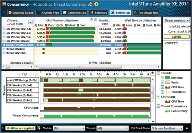
Figure 3.22 Amplifier information showing thread concurrency for the Cilk Plus program

All this Amplifier information shows that the Cilk Plus program is highly efficient and concurrent. As such, no further tuning is required.

Example 2: Working with OpenMP

The following sections assume that you are using the Intel C++ compiler. However, note that Microsoft Visual C++ compiler also supports OpenMP, should you want to use it.

Step 1: Analyze the Serial Program

The analysis step is identical to the one you already did for the Cilk Plus example, so there is no need to do anything else. If you didn't run the first analysis, go to Example 1 and, starting from Listing 3.1, complete the steps outlined in the following sections:

Once you have done these you are ready to start the next section.

Step 2: Implement Parallelism using OpenMP

OpenMP uses pragma directives within existing C++ code to set up parallelism. You can modify the directives using clauses.

To add parallelism to the original serial program of Listing 3.1, follow these steps:

// Work loop, do some work by looping VERYBIG times
#pragma omp parallel for
for( int j=0; j<VERYBIG; j++ )
{

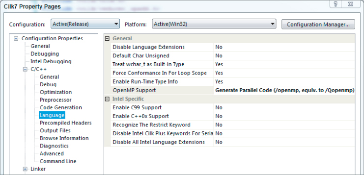
#include <omp.h>

Figure 3.23 Enabling OpenMP in the compiler

When the OpenMP directive is encountered, a parallel region is entered and a pool of threads is created. The number of threads in the pool usually matches the number of cores. Execution of the for loop that follows is parallelized, with its execution being shared between the threads.

Figure 3.24 shows the timings for a 4-core processor. The timings are not very encouraging when compared against the serial timings given in Figure 3.6. And, once again, the Total and Check Sum values are incorrect. As in the Cilk Plus case, the problem is with data races. Remember, your times may be different from those shown here.

Figure 3.24 Timings for the OpenMP parallelized program, initial stage

Step 3: Debug and Check for Errors

An inspection of the threading errors using Intel Parallel Inspector shows the same data race problems occurring as revealed in the Cilk Plus example (refer to Figure 3.15). Remember to limit the activity of the program and build a debug version. The solutions applied to eliminate the data races revealed are similar but work subtly differently from those applied under Cilk Plus. As before, the data races break down into two types: those that can be solved by using private variables, and those that need to use reduction variables. OpenMP can handle both types, but it does so in a different way from Cilk Plus, by using clauses on its directives.

Making the Shared Variables Private

You can fix the data races caused by variables sumx, sumy, and k by creating private variables for each thread by adding a private clause to the parallel pragma directive, as follows:

#pragma omp parallel for 
private( sumx, sumy, k )

The backslash () is used as a continuation marker and its use after the first line is merely to indicate that the directive continues onto the next line. In an OpenMP parallelized for loop, its loop counter is, by default, always made private, which is why it did not show up in the inspection as an extra data race. The variables in the list must already exist as declared nonlocal variables — that is, as automatic, static, or global variables.

When the worker threads are created, they automatically make private versions of all the variables in the private list. During execution each thread uses its own private copy of variables, so no conflicts occur and the data races associated with these variables are resolved.

Adding a Reduction Clause

As with the Cilk Plus solution, a different approach is required for variables within the loop that must be shared by the threads; they cannot be made private. This is handled in OpenMP by adding a reduction clause to the OpenMP directive:

#pragma omp parallel for      
    private( sumx, sumy, k )  
    reduction( +: sum, total )

When the parallel section is reached, each participating thread creates and uses private copies, or versions, of the listed reduction variables. When the parallel section ends, the private thread versions of the variables are operated on according to the operator within the reduction brackets — in this case, they are added together. The resultant value is then merged back into the original nonlocal variable for future use. Other operators, such as multiply and subtract (but not divide), are also allowed. Note that it is up to the programmer to ensure that the operation on the variables within the loop body matches the operator of the reduction clause. In this case, both sum and total are added to each iteration of the work loop, which matches the reduction operator of +.

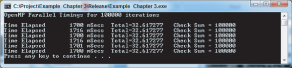
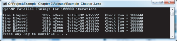
After rebuilding and running the Release version, you should see the times obtained for a 4-core machine (Figure 3.25). This corrects the Check Sum and Total values, but with an average time increase of only 2.28 times that of Figure 3.6. Further tuning is required. Remember, your times may be different, depending on the system you are running.

Figure 3.25 Timings for the OpenMP parallelized program, with private and reduction variables

Step 4: Tune the OpenMP Program

To use Intel Parallel Amplifier XE to check for concurrency and efficiency within the OpenMP program, follow these steps:

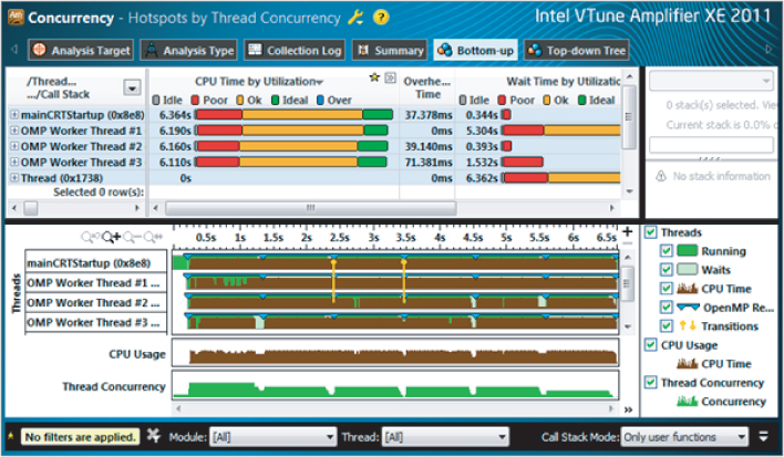
Figure 3.26 Concurrency information showing unbalanced loads

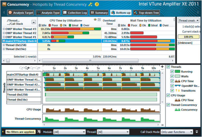
The results are very different from those shown for Cilk Plus. The top pane shows the mainCRTStartup thread, as with the Cilk Plus model, but now there are only three other OMP Worker Threads, numbered 1 to 3 — because the main (serial) thread is also used as one of the parallel threads. This is different from Cilk Plus. Two other threads, created by the operating system, do not take part in the parallel operations and do no work, so you can ignore them.

The top pane, which shows CPU utilization time for each thread, clearly indicates an imbalance between the threads, with the mainCRTStartup thread doing less than a third of the work of OMP Worker Thread 3.

This imbalance is reflected in the lower pane, where the timelines of each of the parallel threads are given. Brown shows when a thread is doing work, and green shows when it is idle. You can clearly see that the mainCRTStartup thread is doing little work compared to the OMP Worker Thread 3. Also notice the same sixfold pattern to the work caused by the outer loop running six times.

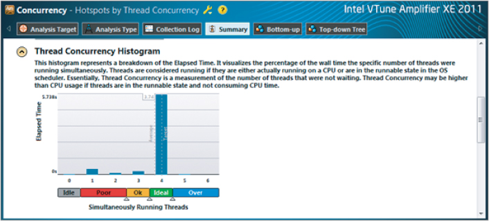
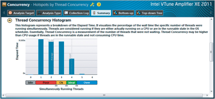
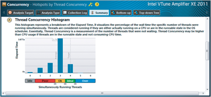
The CPU Usage and Thread Concurrency timelines both show poor performance. This is demonstrated in Figure 3.27, which can be obtained by clicking the Summary button. This shows the amount of time spent with 0, 1, 2, 3, and 4 threads running concurrently. Only a small part of the time are four threads running together, with more than a quarter of the time spent running only a single thread. Overall, an average of 2.26 threads were running concurrently, which agrees almost exactly with the increase in speed.

Figure 3.27 Amplifier showing thread concurrency for the OpenMP program before tuning

The problem occurs because the arithmetic series required more terms as the iteration count of the work loop grew larger. As the work loop counter increases, so too does the amount of work required to calculate the arithmetic series. However, unlike Cilk Plus, the default scheduling operation of OpenMP is to simply divide the execution of the work loop between the available threads in a straightforward fashion. Each thread is given the task of iterating the work loop a fixed number of times, referred to as the chunk size. For example, on a 4-core machine, with an iterative count of 100,000, OpenMP simply divides the iterations of the loop by four equal ranges:

• One thread is given iterations for loop counter 0 to 24,999.
• The next thread is given iterations for loop counter 25,000 to 49,999.
• The next thread is given iterations for loop counter 50,000 to 74,999.
• The final thread is given iterations for loop counter 75,000 to 99,999.

For most purposes, this would be a balanced workload, with each thread doing an equal amount of work. But not in this case. Threads working through higher-value iterations encounter arithmetic series with greater numbers of terms, the number of terms being dependent on the iteration value. This means that the threads working on the higher iterations have to do more work, creating unbalanced loading of the threads.

Figure 3.28 demonstrates a simplified problem with unbalanced loads. In this example a serial program enters a loop with a count of 12, where each iteration of the loop carries out work whose execution takes longer. This is indicated by the blocks marked 1 through 12 on the top bar, labeled Single Thread (78 time units). This bar represents the running of the serial program, where the width of each block is the time taken to execute each of the 12 loops. In this example the first loop takes 1 time unit, the second loop takes 2 time units, and so on, with the final loop taking 12 time units — making a total time of 78 time units to run the serial program.

Figure 3.28 Example demonstrating unbalanced loading

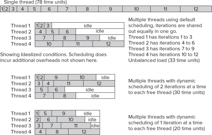
Ideally, the parallelized time to run the same loop on a 4-core machine should be 78/4 = 19.5 time units; however, this is not the full story.

The default scheduling behavior for OpenMP is to distribute the loops equally to all the available threads — in this case, as follows:

• Thread 1 is allocated iterations 1 to 3.
• Thread 2 is allocated iterations 4 to 6.
• Thread 3 is allocated iterations 7 to 9.
• Thread 4 is allocated iterations 10 to 12.

When you run the parallel program under these default conditions, the result is shown by the second block of Figure 3.28. Thread 4 has all the high iterations, which take more time. Thread 4's running time is 10+11+12=33 time units, which is clearly shown in the diagram. Concurrently running thread 3 takes only 7+8+9=24 time units to execute its allocated work. Thread 2 takes 15 time units, and thread 1 takes only 6 time units. Since all threads must synchronize at the end of the parallelized loop before continuing, it means that threads 1 to 3 must wait for thread 4 to complete. A lot of time that could be otherwise used is wasted.

You can alter the scheduling preferences of OpenMP by using the scheduling clause. This clause enables you to set how many iterations each thread will be allocated—referred to as the chunk size. Each thread will execute its allocated iteration of the loop before coming back to the scheduler for more.

The third block of Figure 3.28 shows what happens when a new scheduling preference of 2 is used. At the start of the loop each available thread receives two iterations, as follows:

• Thread 1 is allocated iterations 1 and 2.
• Thread 2 is allocated iterations 3 and 4.
• Thread 3 is allocated iterations 5 and 6.
• Thread 4 is allocated iterations 7 and 8.

In this case thread 1 quickly executes its 2 allocated iterations, taking only 3 time units to do so. It then returns to the scheduler for more, and is given iterations 9 and 10 to execute. Thread 2 also finishes its allocated work, taking 7 time units, before returning back to the scheduler to be given iterations 11 and 12 to execute.

When threads 3 and 4 finish, they also return back to the scheduler, but since there is no more iterations to be executed they are given no more work. These threads must idle until the other threads finish their work. The first thread must also idle for a time since the execution of its allocated iterations finishes before the second thread. All this is clearly shown by the third block of Figure 3.28, where the second thread dictates the overall time of execution — in this case, 30 time units.

The fourth block of Figure 3.28 demonstrates what happens if the chunk size for the scheduler is reduced to just 1. The overall time of execution, decided by the fourth thread, reduces to just 20 time units and minimal idle time.

There is an overhead because scheduling chunks takes time; too small of a chunk size could end up being detrimental to the operation. Only by trying various values can you find the correct chunk size for your particular program.

Improving the Load Balancing

To obtain a balanced load, you need to override the default scheduling behavior. In this case the loop iterates 100,000 times, so as a first attempt use a chunk size of, say, 2000. You can override the default scheduling algorithm for a for loop by using the schedule clause on the directive:

#pragma omp parallel for        
    private( sumx, sumy, k )    
    reduction( +: sum, total )  
    schedule( dynamic, 2000 )

This causes the OpenMP directive to use the fixed chunk size given in parentheses — in this case, 2000. After each thread finishes its chunk of work (2,000 iterations), it comes back for more. This divides the work more evenly. Adjusting the size of the chunk fine-tunes the solution further. The problem of an unbalanced load does not arise with Cilk Plus, because its approach for dividing up the work is different.

After rebuilding the solution with these changes, run Parallel Amplifier again to check for concurrency. Again, select Thread/Function/Call Stack. Figure 3.29 shows the result.

Figure 3.29 Concurrency showing balanced (but still not ideal) loads

The figure shows nicely balanced loads, but the load bars show mainly Ok (orange), not Ideal (green). Figure 3.30 shows the Thread Concurrency Histogram, with the average number of threads running concurrently still only 2.76.

Figure 3.30 Concurrent information after first tuning attempt

You can try tuning further by changing the chunk size to 1000. Figure 3.31 shows the results of the concurrency; clearly, all four threads are running in an Ideal state (green). This is verified in the Thread Concurrency Histogram (Figure 3.32), which shows an average thread concurrency of 3.75 — in line with the speedup shown in Figure 3.33 compared to the serial times given in Figure 3.6.

Figure 3.31 Concurrency showing balanced and ideal loads

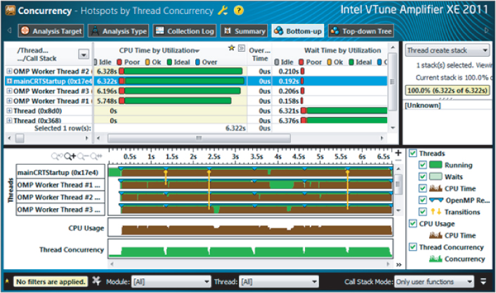
Figure 3.32 Concurrent thread information after final tuning

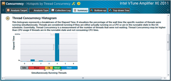
Figure 3.33 Final timings for the OpenMP parallelization

Listing 3.4 gives the final OpenMP program. Its performance compares very well with that achieved using the Cilk Plus method of parallelization.

Listing 3.4: The final version of the OpenMP program

// Example Chapter 3 OpenMP Program
#include <stdio.h>
#include <windows.h>
#include <mmsystem.h>
#include <math.h>
#include <omp.h>

const long int VERYBIG = 100000;

// ***********************************************************************

int main( void )
{
  int i;
  long int j, k, sum;
  double sumx, sumy, total, z;
  DWORD starttime, elapsedtime;

  // ---------------------------------------------------------------------

  // Output a start message
  printf( "OpenMP Parallel Timings for %d iterations 

", VERYBIG );
    
  // repeat experiment several times
  for( i=0; i<6; i++ )
  {
    // get starting time
    starttime = timeGetTime();

    // reset check sum and total
    sum = 0;
    total = 0.0;

    // Work loop, do some work by looping VERYBIG times
    #pragma omp parallel for       
      private( sumx, sumy, k )     
      reduction( +: sum, total )   
      schedule( dynamic, 1000 )
      for( int j=0; j<VERYBIG; j++ )
      {
        // increment check sum
        sum += 1;

        // Calculate first arithmetic series
        sumx = 0.0;
        for( k=0; k<j; k++ )
          sumx = sumx + (double)k;

        // Calculate second arithmetic series
        sumy = 0.0;
        for( k=j; k>0; k-- )
          sumy = sumy + (double)k;

        if( sumx > 0.0 )total = total + 1.0 / sqrt( sumx );
        if( sumy > 0.0 )total = total + 1.0 / sqrt( sumy );
      }

      // get ending time and use it to determine elapsed time
      elapsedtime = timeGetTime() - starttime;

      // report elapsed time
      printf("Time Elapsed %10d mSecs  Total=%lf   Check Sum = %ld
",
                  (int)elapsedtime, total, sum );
  }

  // return integer as required by function header
  return 0;
}

// **********************************************************************

code snippet Chapter33-4.cpp

Summary

The four-step method (analyze, implement, debug, and tune) is used to transform a serial program into a parallel program using the tools of Intel Parallel Studio XE. The technique can be used for small or large programs.

This chapter described using both Intel Cilk Plus and OpenMP to make a serial program parallel. The use of Intel Parallel Studio XE makes the transformation from serial to parallel efficient and effective. The tools also detect both threading and memory errors, and enable you to check a program's concurrency.

Other parallel programming techniques are available and are introduced in subsequent chapters of the book. Which parallelizing methodology is best to use remains the choice of the programmer. That decision can be influenced by many things, including the type of problem being solved, the software tools available, or just what the programmer feels comfortable with.

Part II, “Using Parallel Studio XE,” takes a more detailed look at the four steps. A greater understanding of the pitfalls that can occur when parallelizing will give you much more confidence to tackle large and complex programs, where you can reap the full benefit of using parallel computing. Part II covers each step in turn, revealing the detailed nuances that enable you to undertake efficient and, more important, safe parallelism.