
Chapter 12
Event-Based Analysis with VTune Amplifier XE
What's in This Chapter?
Using the cycles per instruction retired (CPI) metric to spot potentially unhealthy programs
Using Amplifier XE's General Exploration analysis to identify performance issues in your program
Drilling down into architectural hotspots
Using Amplifier XE's APIs to control data collection
When we are ill, most of us know how to check the obvious. Do we have a fever? Are we aching anywhere? Is our pulse rate normal? Wouldn't it be great if there were an easy way of measuring the health of a program? The good news is that some equivalent indicators can be used to monitor the health of an application, and Amplifier XE can be used to get those measurements.
This chapter shows how to check the health of an application using Amplifier XE's architectural analysis types. Starting with a system-wide view of your system, you learn how to observe how well different programs are performing.
Testing the Health of an Application
When looking at the health of an application, several facts need to be ascertained. Like people, each piece of software has its own unique traits. Even if two programs do the same thing — for example, predicting the weather — they may work quite differently internally. These internal differences often have a direct impact on how quickly a program runs and how well the software makes use of the CPU. A well-written “healthy” program will run efficiently, whereas a poorly written “sick” program may run slowly and waste CPU resources.
The following are basic questions to ask when optimizing software:
- How long does the program run?
- How much work does the program do?
- Does the program have any inefficiencies?
Fortunately, all Intel CPUs have hardwired into them electronics that can measure myriad parameters and statistics. Two fundamental parameters (clock ticks and instructions retired), and an associated ratio (cycles per instruction retired), can be used to quickly spot unhealthy software.
- Clock ticks show how many CPU cycles a program consumed. They are a measure of time. Depending on the processor you are running on, clock ticks might be measured per logical core or per CPU.
- Instructions retired measure the number of instructions that have progressed all the way through the CPU pipeline and have not been abandoned along the way. The retired instructions represent the real work being done by the program.
- Cycles per instruction retired (CPI) gives an average figure of how much time each executed instruction took in cycles. The formula is as follows:
CPI = clock tricks / instructions retired
What Causes a High CPI?
In modern CPUs, it is theoretically possible to have four instructions retired on each cycle, giving a CPI of 0.25; however, this low of a figure is rarely achieved. If your application has a CPI of below 1, you are doing pretty well. In the hands-on activities you will see CPI values varying from 26, which is terrible, down to about 0.4, which is excellent.
If you take every cycle of a program, you will find that each cycle can be classed in one of three ways (see Figure 12.1).
- Cycles where instructions are executed and usefully employed (A)
- Cycles where the CPU is doing nothing (B)
- Cycles where instructions are read and possibly executed but are then abandoned or “thrown away” (C)
Figure 12.1 Every cycle the CPU consumes can be categorized based on how they use instructions
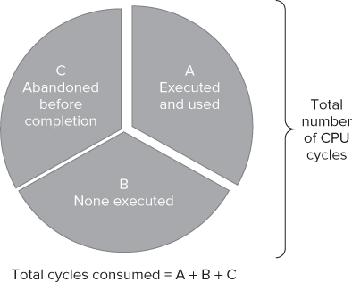
A healthy program will have very few of categories B and C, with most of the cycles being executed and used. An unhealthy program will have a lot of cycles that are not doing anything useful. The more B or C type cycles, the worse the CPI. (Note that the terms A, B, and C have no special significance; they are used merely to help identify the segments in Figure 12.1.)
You will probably find that your application is dominated by one of the segments. You can use Amplifier XE to detect these different cycles by looking for the hotpots in your code.
Is CPI on Its Own a Good Enough Measure of Health?
Although CPI can be used to indicate that some programs have wasted cycles and hence present optimization opprtunities, using just CPI can occasionally be misleading.
In Activities 12-3 and 12-4 later in the chapter, you will see that the speed of the matrix multiplication program improves but the CPI gets worse.
When doing any optimization work, always keep an eye on the most fundamental measurement — that is, how long a program took to run; otherwise, you may spend a lot of unfruitful time improving the CPI but ending up with a slower program.
Conducting a System-Wide Analysis
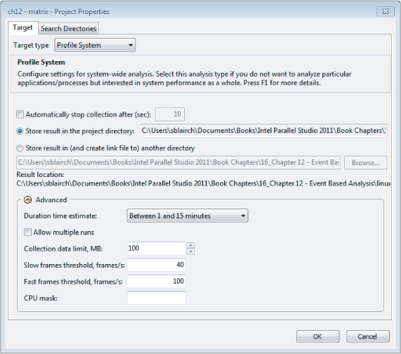
It's sometimes educational to do a system-wide analysis on a PC with Amplifier XE to see which programs have the best CPI and which have the worst. To perform a system-wide analysis, you first set the project properties to Profile System, as shown in Figure 12.2, and then launch a Lightweight Hotspots analysis. This kind of hotspot uses the performance monitoring capabilities of the CPU, has a very low impact on the running programs, and is capable of sampling everything that running on your PC.
Figure 12.2 Editing the project properties to enable system-wide profiling
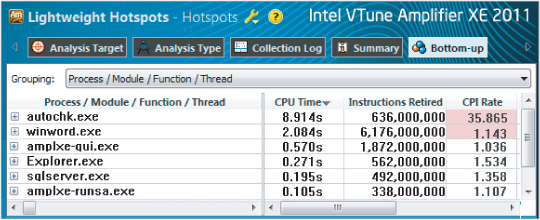
Once you've run a profiling session, you'll probably be fascinated by the results. Figure 12.3 shows the results of doing an analysis on a dual core laptop (the one that was used to write this chapter). Notice that autocheck.exe has a huge CPI of nearly 36. As it happens, this value is expected. Autocheck.exe is part of Windows and is designed to be non-CPU-intensive, running in the background doing some maintenance activities. Amplifier XE highlights the CPIs to alert you to values that need further investigation.
Figure 12.3 A system-wide analysis reveals the CPI rate of every program
Looking at CPI of different programs is entertaining, but there is a serious part to exercise as well. Apart from CPI spotting, you can use the same system-wide analysis to see if one particular program is hogging all the CPU time, as the following story illustrates.
In a recent code-optimization training session at a university, a student complained that his “optimized” applications ran unexpectedly slow. By running a system-wide analysis with Amplifier XE, the reason for the slowdown became obvious. Another user was logged on to the same node and running an MP3 player; the player had been running for the last five days! After a little further exploration, the user of the MP3 software was identified as being someone from the university's IT department. Once the MP3 player was killed, the application ran as expected.
![]()
amplxe-gui
- The application with the largest CPI
- Any fields highlighted in pink
Conducting a Hotspot Analysis
Once it is established that someone is not well, a more detailed diagnosis is needed, with the doctor prodding, poking, and asking appropriate questions. The doctor will need to work out what the problem is in order to decide on the best treatment. Someone complaining of feeling hot and having stomach pain should be dealt with quite differently from someone with a suspected broken leg. Knowing the location and nature of any discomfort or pain is essential for a correct diagnosis.
In the same way, once you've identified that your program is running poorly by looking at the CPI and the time the program took to run, you should conduct a hotspot analysis to find out where the bottlenecks are in your code. After identifying the hotspots, you then need to find the cause of the hotspots and apply suitable remedies.
Hotspot Analysis Types
Amplifier XE has two hotspot analysis types:
- Lightweight Hotspots analysis — This uses hardware event-based sampling and samples all the processes running on a system. The overhead of this type of collection is very low. No stack information is collected in this analysis type. The lightweight hotspot analysis can be applied either to a single application or to the whole system, depending on whether you choose Profile System or Launch Application in the project properties. If you choose Launch Application, only information about the application will be displayed; the rest will be filtered out.
- Hotspots analysis — This employs user-mode sampling and, unlike lightweight hotspots, will collect stack and call tree information. You cannot use this kind of analysis to do a system-wide analysis; it is used to analyze a single application or process. You can find more information on this kind of analysis in Chapter 6, “Where to Parallelize.”
![]()
User Mode Hotspots Versus Lightweight Hotspots
It's worth spending a few minutes looking at the difference between the two types of analysis. The screenshots in this section use the code from matrix.cpp in Listing 12.3 (at the end of the chapter). The machine used has a second-generation Intel Core Architecture (aka Intel Sandy Bridge) 3.0 GHz processor, 8GB of memory running Centos 5 (64-bit 2.6.18 Kernel). The CPU has 4 cores and supports hyper threading, giving a total availability of 8 logical CPUs.
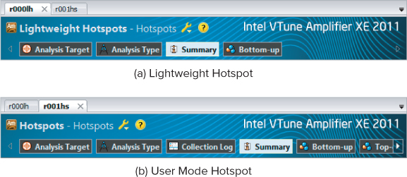
The Results Tabs
Amplifier XE displays the data collected from a hotspot analysis in different tabs (see Figure 12.4). Notice that the User Mode Hotspots analysis has five tabs, whereas the Lightweight Hotspots analysis has only four tabs. The extra tab, Top-down Tree, is available only in the User Mode Hotspots analysis because only this analysis collects stack and call graph information.
Figure 12.4 The results tabs
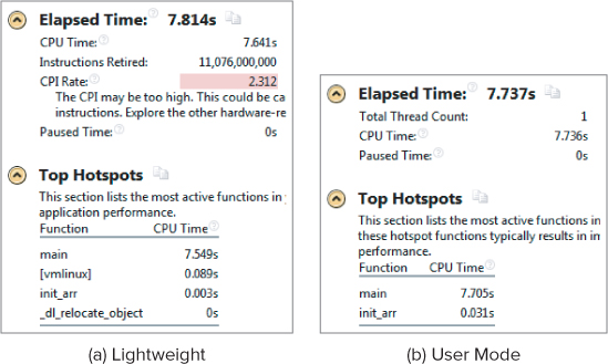
The Summary Tab
When you select the Summary tab, the Lightweight Hotspots analysis gives two extra pieces of information: Instructions Retired and CPI Rate (see Figure 12.5). Notice that the Lightweight Hotspots analysis lists what seems to be two OS-related functions: vmlinux and _dl_relocate_object. The Paused Time records the amount of time the analysis ran with the collector paused.
Figure 12.5 A summary page showing the two types of hotspot analysis
The Bottom-up Tab
You can group and display the results in the Bottom-up tab according to different objects, such as Process, Module, Thread, and so on. Table 12.1 lists the different objects used in the two types of hotspot analysis. Most terms will be familiar to you or will be explained later; however, the following two terms need a quick explanation now:
- Package refers to the physical CPUs. A dual-CPU system has two packages.
- H/W context refers to logical CPUs.
Table 12.1 Objects Used in the Bottom-up Results Grouping
| Object | Lightweight | User Mode |
| Process | Y | N |
| Module | Y | Y |
| Thread | Y | Y |
| Source file | Y | Y |
| Function | Y | Y |
| Basic nlock | Y | N |
| Code location | Y | N |
| Class | Y | Y |
| H/W context | Y | N |
| Package | Y | N |
| Frames | Y | Y |
| Call stack | N | Y |
| OpenMP regions | N | Y |
| Task type | N | Y |
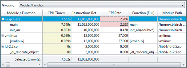
Figure 12.6 shows an example of lightweight hotspots grouped by module/function.
Figure 12.6 Lightweight hotspots grouped by module/function
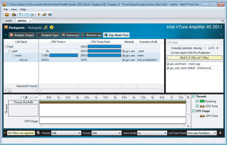
The Top-down Tree Tab
Only the User Mode Hotspots analysis has a top-down view. This view displays the call stack and timeline view as shown in Figure 12.7.
Figure 12.7 The Top-down Tree tab of the User Mode Hotspots analysis
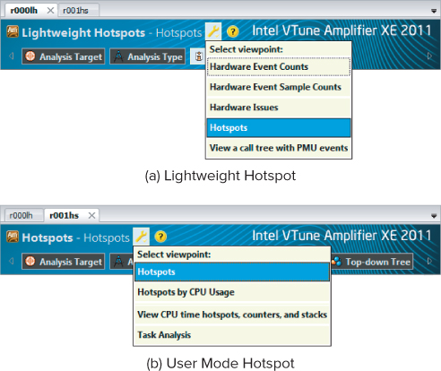
Viewpoints
All analysis types have a default view. You can change the view by clicking the spanner next to the analysis title (see Figure 12.8). The Lightweight Hotspots analysis has four views, whereas the User Mode Hotspots analysis has only two views. Viewpoints are simply different ways of presenting the collected data. Because the User Mode Hotspots analysis does not collect any hardware events, only two viewpoints are available.
Figure 12.8 Different viewpoints for the two types of analysis
To summarize, the major differences between the two types of hotspot analysis are as follows:
- Lightweight Hotspots analysis is system wide but does not collect call stack information. It collects CPU events, and therefore can display metrics such as CPI.
- User Mode Hotspots analysis is not system wide but does provide call stack information. This type of analysis is primarily concerned with the amount of time each part of a program takes. It cannot display events or CPI.
Finding Hotspots in Code
Back to the task at hand. The purpose of doing a hotspot analysis is to determine the health of your code and to understand the nature of any bottlenecks. For this type of analysis you need to use a Lightweight Hotspots analysis rather than a User Mode Hotspots analysis.
As shown in Figure 12.6, the biggest lightweight hotspot in ijk.gcc.exe is the main() function, which is using just over 7.5 seconds of CPU time. This is the sum of how much time each individual hardware thread used. The CPI is 2.293, indicating that there may be a problem. By clicking on the hotspot, you can drill down to the source code (see Figure 12.9).
Figure 12.9 The Source view
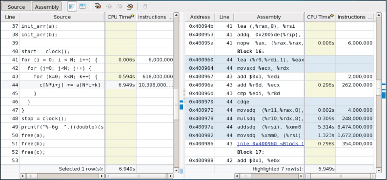
Looking at the C code of the hotspot, you can see that three arrays (a, b, and c) are accessed:
for (i = 0; i < N; i++) {
  for (j=0; j<N; j++) {
    for (k=0; k<N; k++) {
      c[N*i+j] += a[N*i+k] * b[N*k+j];
      // printf("%p,%p,%p
", &c[N*i+j],&a[N*i+k],&b[N*k+j]);
    }
  }
}
The right side of the Source view in Figure 12.9 shows the disassembly window (duplicated in Table 12.2). The instructions that take the most time are addsdq and movsdq.
Table 12.2 The Assembly Lines
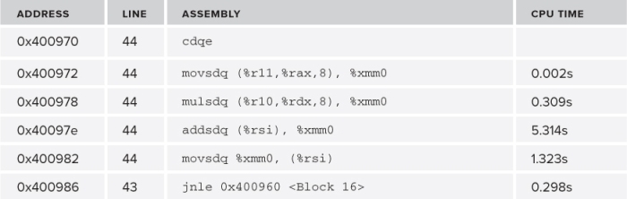
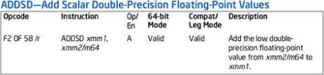
Both of the addsdq and movsdq instructions access memory, so the underlying problem might be related to memory. If you are not an expert on assembler instructions, you can use the online context-sensitive help to display the instruction description, as shown in Figure 12.10.
Figure 12.10 Online instruction help
The code was built as a 64-bit application using GNU GCC version 4.1.2. If you have built a 32-bit application or used a different compiler, you may get different assembler instructions. The events that have been captured do not yet tell exactly what is happening in the CPU, although depending on your profiling experience you might be able to guess as to what the underlying cause is.
Try out a Lightweight Hotspots analysis for yourself using the instructions in Activity 12-2.
Linux
g++ matrix.cpp -g -O2 -o matrix.exe
Windows
cl matrix.cpp /Zi /O2 -o matrix.exe
- The C line taking up the most time
- The assembler instruction taking up the most time
- The CPI rate of the bottleneck
Conducting a General Exploration Analysis
A good doctor will find the underlying cause of an illness. Sometimes the reason will be obvious, and sometimes finding the exact cause will be difficult. You have the same set of challenges when examining your software.
You already know where the bottleneck is, so now you need to dig a little deeper to find out what is causing the hotspot. Amplifier XE's General Exploration analysis is designed to help you do this. The General Exploration analysis looks for hardware issues that can cause problems. Amplifier XE has multiple versions of this analysis type that are dedicated to different CPUs. This chapter uses the version for Intel Microarchitecture Code Name Sandy Bridge. If you use a different version (because your system is from a different CPU family), the results may be categorized differently.
When an analysis has completed, the Bottom-up window is displayed, as shown in Figure 12.11. Several fields are highlighted to draw your attention to potential problems.
Figure 12.11 The Bottom-up window with each issue highlighted
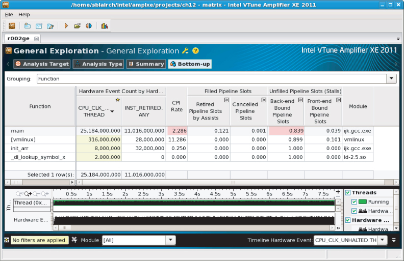
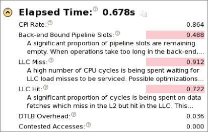
As shown in Figure 12.12, the summary page identifies four hardware issues: CPI Rate, Back-end Bound Pipeline Slots, LLC Miss, and DTLB Overhead. Figure 12.12 shows only the top part of the summary page; more entries are available further down the list, but none of them are highlighted.
![]()
Figure 12.12 A summary of the General Exploration analysis
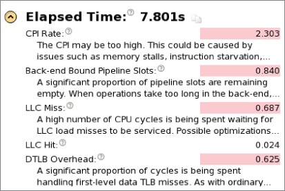
Every ratio, apart from CPI, has a value between 0 and 1. The nearer the value is to 0, the better the performance. Before exploring further what these entries mean, try out Activity 12-3.
Linux
g++ matrix.cpp -g -O2 -o matrix.exe
Windows
cl matrix.cpp /Zi /O2 -o matrix.exe
- Advanced Intel Core 2 Processor Family Analysis
- Advanced Intel Microarchitecture Code Name Nehalem Analysis
- Advanced Intel Microarchitecture Code Name Sandy Bridge Analysis
- Advanced Intel Atom Processor Analysis
A Quick Anatomy Class
One of the most daunting aspects of optimizing code is coming to grips with the internals of the CPU. Fortunately, Amplifier XE helps out by providing predefined analysis types along with helpful on-screen explanatory notes. Here's an example of the explanatory note attached to the CPI ratio:
"Cycles per instruction retired, or CPI, is a fundamental performance metric
indicating approximately how much time each executed instruction took, in units of
cycles. Modern superscalar processors issue up to four instructions per cycle,
suggesting a theoretical best CPI of .25. But various effects (long latency memory,
floating-point, or SIMD operations; nonretired instructions due to branch
mispredictions; instruction starvation in the front-end) tend to pull the observed
CPI up. A CPI of 1 is generally considered acceptable for HPC applications but
different application domains will have very different expected values. Nonetheless,
CPI is an excellent metric for judging an overall potential for application
performance tuning"
CPU Internals
Just as knowing what to call different parts of your anatomy is helpful when describing your aches and pains to the doctor, it is helpful to know a few terms to help describe bottlenecks.
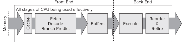
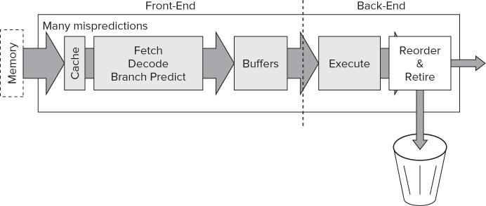
Figure 12.13 shows a high-level view of a typical processor, split into two halves: the front-end and the back-end.
Figure 12.13 The basic blocks of a CPU

The front-end is responsible for the following:
- Fetching instructions from memory.
- Decoding instructions into micro-operations, a format the CPU understands.
- Predicting the direction branch instructions will take and prefetching those instructions ahead of when they are actually needed.
The back-end is responsible for the following:
- Executing the micro-operations. Several execution engines can run in parallel, thus providing instruction-level parallelism. Some engines are dedicated to specific types of instructions.
- Retiring the instructions.
- Preserving the order layout of retired instructions. Some of the micro-operations will be executed out of order. The reorder mechanism makes sure that all retired instructions will be retired in the same order they appeared in the original source code.
The buffers between the front-end and back-end help to mitigate against delays known as stalls. As long as micro-operations are stored in the buffer, even if there is a stall in the front-end, the back-end can still be fed micro-operations from the buffer. This reduces the chance of a front-end stall causing a back-end stall. In fact, many buffers throughout the CPU are not shown in Figure 12.13.
Categories of Execution Behavior
As mentioned previously (in the section “What Causes a High CPI?”), a program's cycles can be split between cycles where something useful is done and cycles where nothing useful is done. The different cycle categories are caused by how the code is executing on the CPU. The categories of execution can be split into the following four types, all of which can indicate that there are tuning optimizations to be had:
- Retirement-dominated execution
- Front-end-bound execution
- Back-end-bound execution
- Cancellation-dominated execution
In each of the following diagrams (Figures 12.14 to 12.17), the flow of instructions through the CPU is shown by the arrow. The thickness of the arrow represents the volume of throughput. Some of the blocks within the diagrams are shaded, which represents a lot of activity (or bottlenecks), whereas others have no shading, which indicates that the blocks are doing very little.
Your program could display all these characteristics in different parts of the program, or it could be dominated by one particular type of behavior.
Retirement-Dominated Execution
In retirement-dominated execution, all the different stages of the CPU are working efficiently with no significant stalls (see Figure 12.14). Typically, the CPI will be low (less than, say, 0.4), and the percentage of CPU utilization will be approaching 100 percent. The main opportunity for optimization is in reducing the amount of code that needs to be executed.
Figure 12.14 Retirement-dominated execution
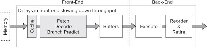
Front-End-Bound Execution
As shown in Figure 12.15, front-end-bound code does not provide enough micro-operations to the back-end. Front-end problems are usually caused by:
- Delays in fetching code — for example, due to instruction cache misses
- Time taken to decode instructions
Figure 12.15 Front-end-bound execution
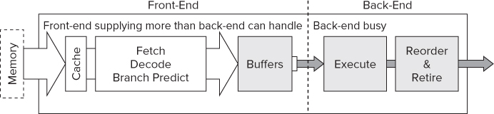
Back-End-Bound Execution
Back-end-bound code is not able to accept micro-operations from the front-end. The front-end supplies more micro-operations than the back-end can handle, leading to the back-end's internal queues being full. This usually is caused by the back-end's data structures being taken up by micro-operations that are waiting for data in the caches.
The hollow arrows in Figure 12.16 are intended to show that the front-end is capable of providing many instructions but cannot because of a busy back-end.
Figure 12.16 Back-end-bound execution
Cancellation-Dominated Execution
In cancellation-dominated execution, many micro-operations are cancelled or “thrown away” (see Figure 12.17). The most common reason for this type of behavior is the front-end mispredicting branch instructions. You often see this kind of behavior in database applications or in code that is doing a lot of pointer chasing, such as in linked lists.
Figure 12.17 Cancellation-dominated execution
Fixing Hardware Issues
An experienced doctor will consider the facts he knows, filter out the unimportant data, and make a diagnosis based on his knowledge and experience. Ideally, after making the right diagnosis, the doctor will procure the correct remedy.
You've seen that Amplifier XE does a great job of collecting the facts and filtering out the unimportant data, eventually coming up with a list of four problems. You probably didn't notice it, but the General Exploration analysis you carried out captured more than 33 different types of events and checked every hotspot against at least 26 different rules.
The next step in the process is to fix the problems identified. It sounds so simple, doesn't it? The question is, which problem should be fixed first? Here are some guidelines that will help you:
- Always fix one problem at a time. Even if you know how to fix more than one problem at once, always focus on just one. Quite often fixing one problem will have a radical effect on other problems; therefore, it's best to go one step at a time, doing a fresh analysis between each fix.
- You can choose in which order to fix the problems either by fixing the problem with the highest ratio or by using Table 12.3, which lists the most common issues in their rough order of likelihood.
Table 12.3 Suggested Order of Fixing Problems
| Priority | Problem | Characteristic |
| 1 | Cache misses | Back-end-bound |
| 2 | Contested access | Back-end-bound |
| 3 | Other data-access issues | Back-end-bound |
| 4 | Allocation stalls | Back-end-bound |
| 5 | Micro assists | Retirement-dominated |
| 6 | Branch mispredictions and machine clears | Cancellation-dominated |
| 7 | Front-end stalls | Front-end-bound |
As shown previously in Figure 12.12, the four problems identified by Amplifier XE are as follows:
- CPI Rate — The high CPI rate is a result of the other hardware issues. Once the issues are fixed, the CPI will drop.
- Back-end-Bound Pipeline Slots — On the machine these tests were run on (a Sandy Bridge), the front-end could provide up to 4 micro-operations per cycle to the back-end. Back-end-bound means the back-end was not able to accept enough operations to match the rate at which the front-end was supplying them.
- LLC Miss — An LLC miss is one of the most common causes of poor performance.
- DTLB overhead — The Data Translation Look-aside Buffer is used to support memory access. Partial copies of this table are normally held in cache. If a program accesses a memory address that is not referenced by the DTLB in cache, the new DTLB entries have to be loaded from external memory, causing a high overhead.
Using Table 12.3 as a guide, the LLC miss is tackled first.
Reducing Cache Misses
The code used for the matrix multiplication, matrix.cpp, is accessing memory in a cache-inefficient way. Figure 12.18 shows two 4x4 matrices, a and b being multiplied together, with the results in matrix c. In Figure 12.18(a) the nested loop uses the variables i, j, and k, with the outermost loop using i, and the innermost loop using k. The diagram shows each of the matrices sitting in the L1 cache and taking up two cache lines.
Figure 12.18 Cache-inefficient and cache-friendly access
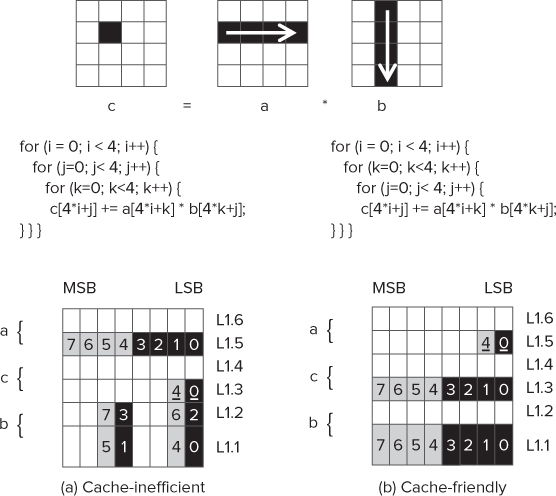
The numbers inside the cells are to show which cell is accessed in each iteration of the nested loop. The underlined numbers represent a sequence of four accesses on the same cell.
In Figure 12.18(a) you can see the following:
- Matrix a is accessed sequentially on each iteration.
- The first cell of matrix c is accessed on loops 0 to 3, and the second cell is accessed on loops 4 to 7.
- The access to the cells of matrix b is not sequential, with the cache line boundary being traversed between alternate loops.
Although this diagram shows only a 4 ×4 matrix, you can imagine that in very large matrices the code in Figure 12.18(a) would result in huge gaps in the address accessed between each read of matrix b, along with cache misses as far back as the Last Level Cache.
You can solve the cache misses by changing the loop sequence so that i and j are swapped. This results in the access to each cell becoming sequential, as shown in Figure 12.18(b).
Rerunning the code with this modification results in the application running much quicker. Table 12.4 shows the results of a General Exploration analysis on the modified application. You can see the following:
- The application runs more than five times faster.
- The CPI rate is much improved.
- The cache misses (LLC) have reduced by a factor of 10.
- The DTLB Overhead likewise is substantially reduced.
- The back-end-bound pipeline slot is reduced by a factor of 5.
- The front-end-bound pipeline slots have increased.
Table 12.4 Comparison of the Original and Loop-swapped Code
| Issue | Original | Swapped |
| Elapsed Time | 7.801 | 1.535 |
| CPI Rate | 2.303 | 0.410 |
| Back-end-Bound Pipeline Slots | 0.84 | 0.159 |
| LLC Miss | 0.687 | 0.073 |
| DTLB Overhead | 0.625 | 0.010 |
| Front-end-Bound Pipeline Slots | 0.040 | 0.163 |
Having fixed the first problem, it's time to move onto the next issue. Although the back-end-bound pipeline slots are much reduced, they are still present and need to be addressed further.
Using More Efficient Instructions
In the assembler view of the application, you may have already noticed that the multiplication is carried out using the mulsd instruction. This instruction is a scalar SSE instruction — that is, it operates only on one value at a time. One way of improving the performance would be to use a packed SSE instruction instead. You can tell whether an instruction is scalar or packed by the presence of the letter s and p in the instruction name. The following code snippet shows packed SSE instructions being used in the inner loop:
for (j=0; j<N; j++) {
        res = _mm_mul_pd(*pA,pB[j]);
        res = _mm_hadd_pd ( res , res);
        _mm_store_sd(&c[N*i+j],res);
      }
By using the packed instruction, there should be a speedup of about two, because packed SSE instructions can calculate two double-precision floating-point values in one instruction.
Listing 12.4 (at the end of the chapter) has a new version of the main() function in which packed SSE instructions have been inserted into the code. Three major changes are made to the code:
- The dynamic allocated memory is aligned to a 16-byte boundary using the _mm_mallocfunction; it is then freed using the _mm_free function.
- Two pointers, pA and pB (of type _m128d), are used to point to the matrices a and b, respectively.
- The calculations are carried out using SSE instructions. The _mm_hadd function performs a horizontal add to add together the results of the vectorized multiplication.
Table 12.5 gives the new results, comparing them to the version that already has its loops swapped. The elapsed time has reduced, but note again that the CPI has increased. The two items in bold are highlighted in pink in Amplifier XE, suggesting that they need further investigation.
Table 12.5 A Comparison of the Loop-swapped and SSE Code
| Issue | Loop-Swapped | SSE |
| Elapsed Time | 1.535 | 0.960 |
| CPI Rate | 0.410 | 0.591 |
| Back-end-Bound-Pipeline Slots | 0.159 | 0.233 |
| LLC Miss | 0.073 | 0.178 |
| DTLB Overhead | 0.010 | 0.016 |
| Front-end-Bound Pipeline Slots | 0.163 | 0.144 |
| Machine Clears | 0 | 0.027 |
Obviously, you still have more opportunities to optimize the code, but rather than using SSE intrinsic functions in your code, it's time to try a different strategy by using the Intel compiler to automatically do the optimizations.
Using the Intel Compiler
Up until now in this chapter, the code has been built with GNU GCC. If you use the Intel compiler, you will find that it automatically does both loop swapping and uses SSE instructions. Figure 12.19 shows the results of building Listing 12.3 with the Intel compiler. The first thing to notice is that the speed has improved yet again, even though the CPI got worse.
Figure 12.19 The results using the Intel compiler
Amplifier XE has identified that there is still more optimization work that could be explored. Because this chapter is mainly about using Amplifier XE, the optimization effort will not be pursued anymore here. If you want to consider some more optimization techniques, refer to Chapter 4, “Producing Optimized Code.”
Implementing Loop Swapping
// do the matrix calculation c = a * b
  for (i = 0; i < N; i++) {
    for (k=0; k<N; k++) {
                for (j=0; j<N; j++) {
                           c[N*i+j] += a[N*i+k] * b[N*k+j];
                         }
             }
  }
Linux
g++ swapped.cpp -g -O2 -o swapped.exe
Windows
cl swapped.cpp /Zi /O2 -o swapped.exe
Using SSE Instructions to Speed Up the Code
Linux
g++ sse.cpp -msse3 -g -O2 -o sse.exe
Windows
cl sse.cpp /Zi /O2 -o sse.exe
Using the Intel compiler
Linux
icc matrix.cpp -g -O2 -o intel.exe
Windows
icl matrix.cpp /Zi /O2 -o intel.exe
Using Amplifier XE's Other Tools
Like all good doctors, you will want to use a choice of instruments to help diagnose an unhealthy application. Amplifier XE's bag of instruments includes:
- Predefined analysis types
- Viewpoints
- APIs
- Command-line interface
- Context-sensitive help and Internet-based resources
Using Predefined Analysis Types
You've already seen how the clock ticks, the number of instructions retired, and the CPI can be gathered from a Lightweight Hotspots analysis. You've also used the General Exploration analysis to spot issues in your code. To do a yet more detailed examination of your program, you can use one of the other predefined analysis types.
A CPU can generate hundreds of different types of events. Using Amplifier XE's predefined analysis types takes the pain out of choosing the right events. Table 12.6 shows the analysis types available.
Table 12.6 Predefined Analysis Types for CPU Architecture-level Analysis
| Analysis | Description |
| General Exploration | As the starting point for advanced analysis, identifies and locates the most significant hardware issues that affect performance |
| Memory Access | Identifies where memory access issues affect performance |
| Cycles and uOps | Identifies where micro-operation flow issues affect performance |
| Bandwidth | Identifies where memory bandwidth issues affect performance |
| Bandwidth Breakdown | Identifies where memory bandwidth issues affect performance; transactions are broken down into reads and write backs |
| Front End Investigation | Identifies where front-end issues affect performance |
| Custom designed | Enables you to create your own analysis type based on any of the predefined types |
Using Viewpoints
Amplifier XE has a number of different viewpoints that represent the results of an analysis. The name of the current viewpoint is displayed in the results tabs, just after the name of the analysis type. Figure 12.20 shows the viewpoint menu, which you can access by clicking on the spanner icon.
Figure 12.20 Changing the viewpoint
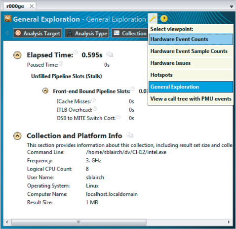
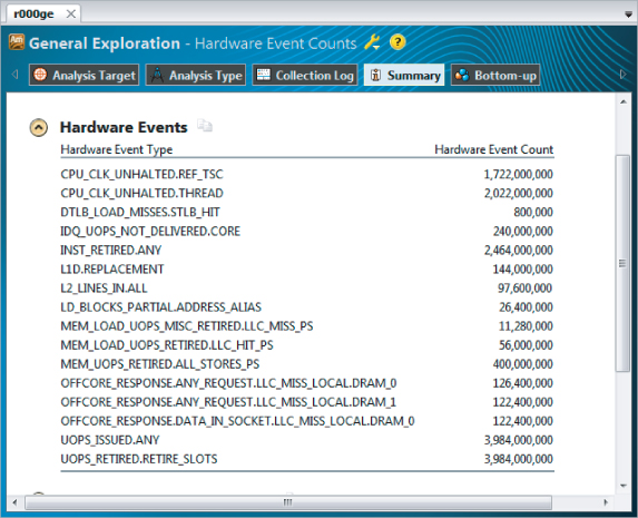
Sometimes it is worth switching between the different viewpoints. For example, while in the General Exploration viewpoint, you might want to see the actual event counts by flipping to the Hardware Event Counts viewpoint. Figure 12.21 shows the summary page of such a viewpoint. In the different viewpoints Amplifier XE uses the existing data but presents it in a different layout. No data is lost or has to be resampled as you swap between viewpoints.
Figure 12.21 The Hardware Event Counts viewpoint
Using APIs
Amplifier XE has a number of APIs that you can insert into a program to control an analysis. Table 12.7 lists some of the commonly used APIs when doing an event-based analysis. Some additional user-mode APIs are also available, which have already been described in earlier chapters.
![]()
Table 12.7 Supported APIs
| Pause/Resume API | Description |
| _itt_pause | Inserts a pause command so that application continues to run but no profiling information is being collected. |
| _itt_resume | Inserts a resume command so that the application continues to run and profiling information is collected. |
| Frame APIs | |
| _itt_domain_create | Creates a domain to hold frame data. You can create multiple domains to help you separate the data into distinct groupings in the GUI. |
| _itt_frame_begin_v3 | Marks the start of a frame. |
| _itt_frame_end_v3 | Marks the end of a frame. |
You can use the Pause and Resume API to turn data collection off and on, respectively, from within the application under test. The Frame API is used to measure the time between two markers, or frames. Use the Frame API when you want to get accurate timing information between two positions in your source code.
The Pause and Resume API
Listing 12.1 uses the _itt_pause() and _itt_resume() functions to pause and resume the data collection, respectively. The code consists of two functions, LoopOne() and LoopTwo(). The content of these functions is not important; they are added simply to make the example run long enough when profiling. The ITT_PAUSE and ITT_RESUME user-defined macros are used to include and exclude the API from the code, depending on whether or not the USE_API macro is defined.
 Listing 12.1: An example of using the Pause and Resume API
#include <stdio.h>
#define USE_API
#ifdef USE_API
#include "ittnotify.h"
#define ITT_PAUSE  _itt_pause()
#define ITT_RESUME _itt_resume()
#else
#define ITT_PAUSE
#define ITT_RESUME
#endif

int LoopTwo(){int i;for (i = 0 ; i < 100000000; i++);return i;}

int LoopOne(int i)
{
      i++;
      if (i > 50)
            return i;
      for (int j = 0 ; j < 10000000; j++);
      return LoopOne(i);
}

int main(int argc, char * argv[])
{
      int a,b;
      ITT_PAUSE;        // start paused

      a = LoopOne(0);
      printf("LoopOne Returns %d
",a);

      ITT_RESUME;       // collect data

      b = LoopTwo();
      printf("LoopTwo Returns %d
",b);
      ITT_PAUSE;        // pause data collection

      return a + b;
}
code snippet Chapter1212-1.cpp
If you try to build this code, you must add libittnotify.lib, which you can find in the Amplifierlib32 or Amplifierlib64 folders. Use the lib64 version if you are building a 64-bit application; otherwise, use the lib32 version.
You can use the Pause and Resume API to reduce the amount of data you collect. Table 12.8 shows the total size of the data collected with and without the pause/resume.
Table 12.8 Amount of Data Collected when Profiling Listing 12.1
| Method | Data Size |
| No pauses | 92.2k |
| With pauses/resumes | 42.0k |
The Frame API
Frame rate analysis was added to Amplifier XE to help game programmers analyze how many frames or pictures are being displayed per second. Although developed with game programmers in mind, the Frame API can be applied to any piece of code. Listing 12.2 shows a loop that iterates 100,000 times — this is the frame in this example. Within the loop, two delays are inserted to simulate frames with different amounts of time.
Listing 12.2: An example of using the Frame API
#include <ittnotify.h>
int main()
{
  _itt_domain* pD = _itt_domain_create( "Time" );
  pD->flags = 1; // enable domain

  for(int i = 0; i < 100000; i++)
  {
    // mark the beginning of the frame
    _itt_frame_begin_v3( pD,NULL);

    // simulate frames with different timings
    if(i%3)
      for(int j = 0; j < 30000; j++);  // a delay
    else
      for(int j = 0;  j < 11200; j++);  // another delay

    // mark the end of the frame
    _itt_frame_end_v3( pD,NULL);
  }
  return 0;
}
code snippet Chapter1212-2.cpp
On Windows the program can be built using the following command:
cl /Od /Zi main.cpp -I"%VTUNE_AMPLIFIER_XE_2011_DIR%include"
"%VTUNE_AMPLIFIER_XE_2011_DIR%/lib64/libittnotify.lib"
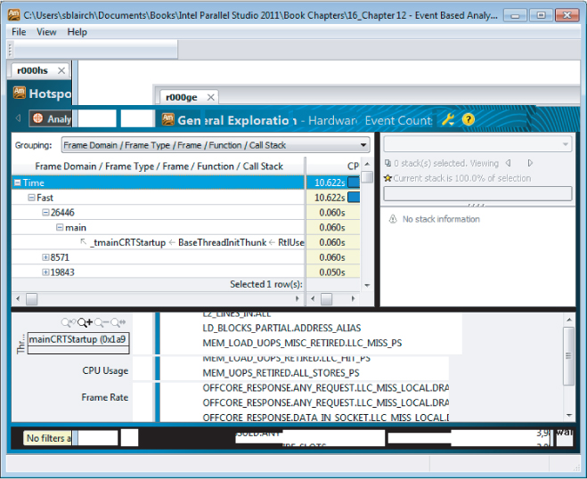
Figure 12.22 shows a zoomed-in view of the analysis. In the timeline view there is an extra bar that displays the frame rate. At the top of the timeline, each frame is marked with a blue line. The Bottom-up pane is organized by Frame Domain/Frame Type/Frame Function. Notice that Amplifier XE splits the frames into fast and slow frames.
![]()
Figure 12.22 An example frame analysis
Using Amplifier XE from the Command Line
You can use the command-line interface (CLI) to Amplifier to collect, compare, and view profiling data. The tool uses the same data collector as the GUI version, so the data collected has the same level of detail as if the profiling were launched from the GUI. The CLI was designed so that Amplifier could be used in scripted and automated test environments.
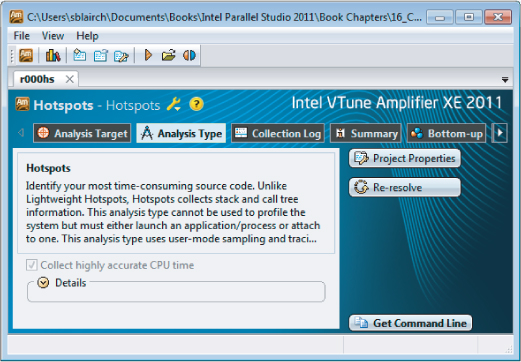
You can generate a command line from an existing project by clicking the Get Command Line button in the Analysis Type window (see Figure 12.23).
Figure 12.23 An Analysis Type window with the Get Command Line button
Here's the command-line syntax:
ampl-cl <action-option> [modifier-options] [[--] <target> [target-options]]
- <action-option> is the action Amplifier XE performs — for example, collecting data or generating a performance report.
- [modifier-options] are various command-line options defining the action.
- <target> is the application to analyze.
- [target options] are the options of the analyzed application.
So, for example:
$ ampl-cl -collect hotspots -r r001hs -- C: estexample.exe
- -collect is an action.
- hotspots is an argument of the action option.
- -r is a modifier option.
- r001hs is an argument of modifier option.
- C: estexample.exe is the target.
- If you have correctly installed Parallel Studio XE, the command ampl-xe should be available from the Parallel Studio XE command prompt (Windows) and the command shell (Linux).
Finding More Information
Here are some resources that you might find helpful:
- The online help that comes with Amplifier XE
- Intel 64 and IA-32 Architectures Software Developers Manuals (www.intel.com/products/processor/manuals)
- The Software Optimization Cookbook, Second Edition: High-Performance Recipes for IA-32 Platforms, by Richard Gerber et al. (www.intel.com/intelpress)
- VTune Performance Analyzer Essentials: Measurement and Tuning Techniques for Software Developers, by James Reinders (www.intel.com/intelpress)
- User forums, such as at http://software.intel.com/en-us/forums/intel-vtune-performance-analyzer
The Example Application
Listing 12.3: matrix.cpp
//Naive matrix multiply
//Warning, this implementation is SLOW!
#include <stdio.h>
#include <time.h>
#include <stdlib.h>

#define DEFAULT_SIZE 1000

// pointers for matrices
double *a, *b, *c;
int N;  // stores width of matrix(if N = 2, then matrix will be 2 * 2)

// function prototypes
void init_arr(double a[]);
void print_arr(char* name, double array[]);
void zero_arr(double a[]);
int main(int argc, char* argv[])
{
  clock_t start, stop;
  int i,j,k;

  // if user does not input matrix size, DEFAULT_SIZE is used
  if(argc == 2)
  {
    N = atoi(argv[1]);
  }
  else
  N = DEFAULT_SIZE;

  // allocate memory for the matrices
  a = (double *)malloc(sizeof (double) * N * N);
  if(!a) {printf("malloc a failed!
");exit(999);}

  b = (double *)malloc(sizeof (double) * N * N);
  if(!b) {printf("malloc b failed!
");exit(999);}

  c = (double *)malloc(sizeof (double) * N * N);
  if(!c) {printf("malloc c failed!
");exit(999);}

  init_arr(a);
  init_arr(b);
  zero_arr(c);

  start = clock();

  // do the matrix calculation c = a * b
  for (i = 0; i < N; i++) {
    for (j=0; j<N; j++) {
       for (k=0; k<N; k++) {
         c[N*i+j] += a[N*i+k] * b[N*k+j];
       }
    }
  }
  stop = clock();

  // print how long program took.
  printf("%-6g  ",((double)(stop - start)) / CLOCKS_PER_SEC);

  // free dynamically allocated memory
  free(a);
  free(b);
  free(c);
}

// print out a matrix
void print_arr(char * name, double array[])
{
  int i,j;
  printf("
%s
",name);
  for (i=0;i<N;i++){
    for (j=0;j<N;j++) {
       printf("%g	",array[N*i+j]);
    }
    printf("
");
  }
}

// initialize array to values between 0 and 9
// this is just to make the printout look better
void init_arr(double a[])
{
  int i,j;
  for (i=0; i< N;i++) {
    for (j=0; j<N;j++) {
      a[i*N+j] = (i+j+1)%10;
    }
  }
}
// initialize array entries to zero
void zero_arr(double a[])
{
  int i,j;
  for (i=0; i< N;i++) {
    for (j=0; j<N;j++) {
      a[i*N+j] = 0;
    }
  }
}
code snippet Chapter12matrix.cpp
Listing 12.4: Using SSE instructions to optimize calculations
// This code should be used to replace the function main()
// from Listing 12-3.
// NOTE: this is not the BEST solution! The best solution is
// simply to build the original code with the Intel Compiler.

// We need some additional headers
#ifdef _WIN32
  #include <intrin.h>
#else
  #ifndef _INTEL_COMPILER
    #include <pmmintrin.h>
  #else
    #include <xmmintrin.h>
  #endif
#endif

int main(int argc, char* argv[])
{
      clock_t start, stop;
      int i, j,k;

  if(argc == 2)
  {
    N = atoi(argv[1]);
  }
  else
    N = DEFAULT_SIZE;

  // printf("Using Size %d
", N);
  a = (double *)_mm_malloc(sizeof (double) * N * N,16);
  if(!a) {printf("malloc a failed!
");exit(999);}

  b = (double *)_mm_malloc(sizeof (double) * N * N,16);
  if(!b) {printf("malloc b failed!
");exit(999);}

  c = (double *)_mm_malloc(sizeof (double) * N * N,16);
  if(!c) {printf("malloc c failed!
");exit(999);}

  init_arr(a);
  init_arr(b);
  zero_arr(c);

  _m128d *pA;
  _m128d *pB;
  start = clock();

  for (i = 0; i < N; i++) {
    for (k=0; k<N; k+=2) {
      pA=(_m128d *)&a[N*i+k];
      pB =(_m128d *)&b[N*k];
      _m128d res = _mm_setzero_pd();
      for (j=0; j<N; j++) {
        res = _mm_mul_pd(*pA,pB[j]);
        res = _mm_hadd_pd ( res , res);
        _mm_store_sd(&c[N*i+j],res);
      }
    }
  }
  stop = clock();
  printf("%-6g  ",((double)(stop - start)) / CLOCKS_PER_SEC);

  _mm_free(a);
  _mm_free(b);
  _mm_free(c);
}
code snippet Chapter1212-4.cpp
Summary
Detecting the health of a program is not easy. Amplifier XE is a very powerful tool, which you can use to find out how well your program is using the CPU.
By first running a system-wide analysis on your PC, you can see how well your program interacts with its environment. You can use the CPI rate as a first indicator of your program's health. Programs with a poor CPI rate are likely to be good candidates for optimization.
Performing a hotspot analysis will show you where the bottlenecks are. You can then use some of the Amplifier XE's predefined analysis types to get more detailed information about the bottlenecks you have discovered.
Amplifier XE's predefined analysis types helps you spot unhealthy code. By becoming aware of the underlying hardware issues in the various bottlenecks of your code, you can begin to address the problems.
Chapter 13, “The World's First Sudoku ‘Thirty Niner,’” is the first of five case studies that show examples of how Intel Parallel Studio XE has been used in different projects.