Discrete signals and systems
2.1 CHAPTER PREVIEW
In this chapter we will look more deeply into the nature and properties of discrete signals and systems. We will first look at a way of representing discrete signals in the time domain. You will then be introduced to the z-transform, which will allow us to move from the time domain and enter the z-domain. This very powerful transform is to discrete signals what the Laplace transform is to continuous signals. It allows us to analyse and design discrete systems much more easily than if we were to remain in the time domain. Recursive and non-recursive filters will be revisited in this new domain. We will also look at how the software package, MATLAB, can be used to help with the analysis of discrete processing systems.
2.2 SIGNAL TYPES
Before we start to look at discrete signals in more detail, it’s worth briefly reviewing the different categories of signals.
Continuous-time signals
This is the type of signal produced when we talk or sing, or by a musical instrument. It is ‘continuous’ in that it is present at all times during the talking or the singing. For example, if a note is played near a microphone then the output voltage from the microphone might vary as shown in Fig. 2.1. Clearly, continuous does not mean that it goes on for ever! Other examples would be the output from a signal generator when used to produce sine, square, triangular waves etc. They are strictly called continuous-time, analogue signals.

Figure 2.1
Discrete-time signals
These, on the other hand, are defined at particular or discrete instants only – they are usually sampled signals. Some simple examples would be the distance travelled by a car, atmospheric pressure, the temperature of a process, audio signals, but all recorded at certain times. The signal is often defined at regular time intervals. For example, atmospheric pressure might be sampled at the same time each day (Fig. 2.2), whereas an audio signal would obviously have to be sampled much more frequently, perhaps every 10 µs, in order to produce a reasonable representation of the signal. (The audio signal could contain frequency components of up to 20 kHz and so, to prevent aliasing, it must be sampled at a minimum of 40 kHz, i.e. at least every 25 µs.)

Figure 2.2
Digital signals
This term is used to describe a discrete-time signal where the sampled, analogue values have been converted to their equivalent digital values. For example, if the pressure values of Fig. 2.2 are to be automatically processed by a computer then, clearly, they will first need to be changed to equivalent voltage values by means of a suitable transducer. An ADC is then needed to convert the resulting voltages to a series of digital values. It is this series of numbers that constitutes the digital signal.
2.3 THE REPRESENTATION OF DISCRETE SIGNALS
Before we can start to consider discrete signal processing in detail, we need to have some shorthand way of describing our signal. Continuous signals can usually be represented by continuous mathematical expressions. For example, if a signal is represented by y = 3 sin 4t, then you will recognize this as representing a sine wave having an angular frequency, ω, of 4 rad/s, and an amplitude of 3. If the signal had been expressed as y = 3e–2t sin 4t, then this is again the same sinusoidal variation but the signal is now decaying exponentially with time. More complicated continuous signals, such as speech, are obviously much more difficult to express mathematically, but you get the point.
Here we are mainly interested in discrete-time signals, and these are very different, in that they are only defined at particular times. Clearly, some other way of representing them is needed. If we had to describe the regularly sampled signal shown in Fig. 2.3, for example, then a sensible way would be as ‘x[n] = 1, 3, 2, 0, 2, 1’. This method is fine and is commonly used. x[n] indicates a sequence of values where n refers to the nth position in the sequence. So, for this particular sequence, x[0] = 1, x[1] = 3, x[2] = 2, and so on.

Figure 2.3
Some simpler signals can be expressed more succinctly. For example, how about the sampled or discrete unit step shown in Fig. 2.4? Using the normal convention, we could represent this as x[n] = 1, 1, 1, 1, 1, 1, …. However, as the ‘1’ continues indefinitely, a neater way would be as:

Figure 2.4
‘x[n]= 1 for n ≥ 0, else x[n] = 0’
In other words, x[n] = 1 for n is zero or positive and is zero for all negative n values.
Because of its obvious similarity to the continuous unit step, which is usually indicated by u(t), the discrete unit step is often represented by the special symbol u[n]:
Another simple but extremely important discrete signal is shown in Fig. 2.5. This is the unit sample function or the unit sample sequence, i.e. a single unit pulse at t = 0. (The importance of this signal will be explained in a later chapter.)

Figure 2.5
This sequence could be represented by x[n] = 1, 0, 0, 0, 0, … or, more simply, by:
This particular function is equivalent to the unit impulse or the Dirac delta function, δ(t), from the ‘continuous’ world and is often called the Kronecker delta function or the delta sequence. Because of this similarity it is very sensibly represented by the symbol δ[n]:
A delayed unit sample/delta sequence, for example, one delayed by two sample periods (Fig. 2.6) is represented by δ[n − 2] where the ‘–2’ indicates a delay of two sample periods.
Beware! It might be tempting to use δ[n + 2] instead of δ[n − 2], and this mistake is sometimes made. To convince yourself that this is not correct, you need to start by looking at the original, undelayed sequence. Here it is the zeroth term (n = 0) which is 1, i.e. δ[0] = 1.

Figure 2.6
Now think about the delayed sequence and look where the ‘1’ is. Clearly, this is defined by n = 2. So, if we now substitute n = 2 into δ[n − 2], then we get δ[2 − 2], i.e. δ[0]. So, once again, δ[0] = 1. On the other hand if, in error, we had used ‘δ[n + 2]’ to describe the delayed delta sequence, then this is really stating that δ[4] = 1, i.e. that it is the fourth term in the original, undelayed delta sequence which is 1. This is clearly nonsense. Convinced?

Example 2.1
An exponential signal, x(t) = 4e–2t, is sampled at a frequency of 10 Hz, beginning at time t = 0.
(a) Express the sampled sequence, x[n], up to the fifth term.
(b) If the signal is delayed by 0.2 s, what would now be the first five terms?
(c) What would be the resulting sequence if x[n] and the delayed sequence of (b) above are added together?
(a) As the sampling frequency is 10 Hz, then the sampling period is 0.1 s. It follows that the value of the signal needs to be calculated every 0.1 s, i.e.:

(b) If the signal is delayed by 0.2 s, i.e. two samples, then the first two samples will be 0,
(c) As x[n] = 4.00, 3.27, 2.68, 2.20, 1.80, 1.47, … and x[n − 2] = 0, 0, 4.00, 3.27, 2.68
2.4 SELF-ASSESSMENT TEST
1. A signal, given by x(t) = 2 cos(3πt), is sampled at a frequency of 20 Hz, starting at time t = 0.
(a) Is the signal sampled frequently enough? (Hint: ‘aliasing’)
(b) Find the first six samples of the sequence.
(c) Given that the sampled signal is represented by x[n], how could the above signal, delayed by four sample periods, be represented?
2. Two sequences, x[n] and w[n], are given by 2, 2, 3, 1 and −1, −2, 1, −4 respectively. Find the sequences corresponding to:
3. Figure 2.8 shows a simple digital signal processor, the T block representing a signal delay of one sampling period. The input sequence and the weighted, delayed sequence at A are added to produce the output sequence y[n].

Figure 2.8
2.5 RECAP
• A sampled signal can be represented by x[n] = 3, 5, 7, 2, 1, … for example, where 3 is the sample value at time = 0, 5 at time = T (one sampling period), etc. If this signal is delayed by, say, two sampling periods, then this would be shown as x[n − 2] = 0, 0, 3, 5, 7, 2, 1, …
• Important discrete signals are the discrete unit step u[n] (1, 1, 1, 1, …) and the unit sample sequence, or delta sequence, δ[n] (1, 0, 0, 0, …).
• Sequences can be delayed, scaled, added together, subtracted from each other, etc.
2.6 THE z-TRANSFORM
So far we have looked at signals and systems in the time domain. Analysing discrete processing systems in the time domain can be extremely difficult. You are probably very familiar with the Laplace transform and the concepts of the complex frequency s and the ‘s-domain’. If so you will appreciate that using the Laplace transform, to work in the s-domain, makes the analysis and design of continuous systems much easier than trying to do this in the time domain. Working in the time domain can involve much unpleasantness such as having to solve complicated differential equations and also dealing with the process of convolution. These are activities to be avoided if at all possible!
In a very similar way the z-transform will make our task much easier when we have to analyse and design discrete processing systems. It takes a process, which can be extremely complicated, and converts it to one that is surprisingly simple – the beauty of the simplification is always impressive to me!
The z-transform, X(z), of x[n] is defined as:
In other words, we sum the expression, x[n]z–n for n values between n = 0 and ∞.
(The origin of this transform will be explained in the next chapter.)
Expanding the summation makes the definition easier to understand, i.e.:
As an example of the transformation, let’s assume that we have a discrete signal, x[n], given by x[n] = 3, 2, 5, 8, 4. The z-transform of this finite sequence can then be expressed as:
Very simply, we can think of the ‘z–n’ term as indicating a time delay of n sampling periods. For example, the sample of value ‘3’ arrives first at t = 0, i.e. with no delay (n = 0 and z0 = 1). This is followed, one sampling period later, by the ‘2’, and so this is tagged with z–1 to indicate its position in the sequence. Similarly the value 5 is tagged with z–2 to indicate the delay of two sampling periods. (There is more to the z operator than this, but this is enough to know for now.)
Example 2.2
Transform the finite sequence x[n] = 2, 4, 3, 0, 6, 0, 1, 2 from the time domain into the z-domain, i.e. find its z-transform.
Example 2.4
Find the z-transform for the discrete unit step, i.e. u[n] = 1, 1, 1, 1, 1, 1, …
N.B. The z-transform of the unit step can be expressed in the ‘open form’ shown above, and also in an alternative ‘closed form’.
The equivalent closed form is
It is not obvious that the open and closed forms are equivalent, but it’s fairly easy to show that they are.
First divide the top and bottom by z, to give
The next stage is to carry out a polynomial ‘long division’:

This gives, 1 + z–1 + z–2 + …, showing that the open and closed two forms are equivalent.
2.7 z-TRANSFORM TABLES
We have obtained the z-transforms for two important functions, the unit sample function and the unit step – others are rather more difficult to derive from first principles. However, as with Laplace transforms, tables of z-transforms are available. A table showing both the Laplace and z-transforms for several functions is given in Appendix A. Note that the z-transforms for the unit sample function and the discrete unit step agree with our expressions obtained earlier – which is encouraging!
2.8 SELF-ASSESSMENT TEST
1. By applying the definition of the z-transform, find the z-transforms for the following sequences:
(b) x[n] = n/(n + l)2 for 0 ≤ n ≤ 3;
(c) the sequence given in (a) above but delayed by two sample periods;
2. Given that the sampling frequency is 10 Hz, use the z-transform table of Appendix A to find the z-transforms for the following functions of time, t:
2.9 THE TRANSFER FUNCTION FOR A DISCRETE SYSTEM
As you are probably aware, if X(s) is the Laplace transform of the input to a continuous system and Y(s) the Laplace transform of the corresponding output (Fig. 2.9), then the system transfer function, T(s), is defined as:
In a similar way, if the z-transform of the input sequence to a discrete system is X(z) and the corresponding output sequence is Y(z) (Fig. 2.10), then the transfer function, T(z), of the system is defined as:
The transfer function for a system, continuous or discrete, is an extremely important expression as it allows the response to any input sequence to be derived.

Figure 2.9

Figure 2.10
Example 2.5
If the input to a system, having a transfer function of (1 + 2z–1 − z–2), is a discrete unit step, find the first four terms of the output sequence.


Example 2.6
When a discrete signal 1, −2 is inputted to a processing system the output sequence is 1, −5, 8, −4.


Example 2.7
A processor has a transfer function, T(z), given by T(z) = 0.4/(z − 0.5). Find the response to a discrete unit step (first four terms only).
Solution: We could solve this one in a similar way to the previous example, i.e. by first dividing 0.4 by (z − 0.5) to get the first four terms of the open form of the transfer function, and then multiplying by 1 + z–1 + z–2 + z–3. If you do this you should find that the output sequence is 0, 0.4, 0.6, 0.7, to four terms.
However, there is an alternative approach, which avoids the need to do the division. This method makes use of the z-transform tables to find the inverse z-transform of Y(z).
Using the closed form, z/(z − 1), for u(z), we get:
We now need to find the inverse z-transform. The first thing we must do is use the method of partial fractions to change the format of Y(z) into functions which appear in the transform tables. (You might have used this technique before to find inverse Laplace transforms.) For reasons which will be explained later, it’s best to find the partial fractions for Y(z)/z rather than Y(z). This is not essential but it does make the process much easier. Once we have found the partial fractions for Y(z)/z all we then need to do is multiply them by z, to get Y(z):

Using the ‘cover-up rule’, or any other method, you should find that A = 0.8 and B = −0.8.

Now z/(z − 1) is the z-transform of the unit step, and so 0.8z/(z − 1) must have the inverse z-transform of 0.8, 0.8, 0.8, 0.8, ….
The inverse transform of 0.8z/(z − 0.5) is slightly less obvious. Looking at the tables, we find that the one we want is z/(z − e–aT).
Comparing with our expression, we see that ![]() . The function z/(z − e–aT) inverse transforms to e–aT or, as a sampled signal, to e–anT. As
. The function z/(z − e–aT) inverse transforms to e–aT or, as a sampled signal, to e–anT. As ![]() , then our function must inverse transform to 0.8(0.5n), i.e. to 0.8(0.50, 0.51, 0.52, 0.53, …) or 0.8, 0.4, 0.2, 0.1, to four terms.
, then our function must inverse transform to 0.8(0.5n), i.e. to 0.8(0.50, 0.51, 0.52, 0.53, …) or 0.8, 0.4, 0.2, 0.1, to four terms.
Subtracting this sequence from the ‘0.8’ step, i.e. 0.8, 0.8, 0.8, …, gives the sequence of 0, 0.4, 0.6, 0.7, … to four terms.
N.B.1. If we had found the partial fractions for Y(z), rather than Y(z)/z, then these would have had the form of b/(z − 1), where b is a number. However, this expression does not appear in the z-transform tables. This isn’t an insurmountable problem but it is easier to find the partial fractions for Y(z)/z and then multiply the resulting partial fractions by z to give a recognizable form.
N.B.2. It would not have been worth solving Example 2.5 in this way, as it would have involved much more work than the method used. However, it is worth ploughing through it, just to demonstrate the technique once again.
The transfer function here is 1 + 2z–1 − z–2 and the input a unit step:
or
i.e.
You should find that this gives A = 2, B = −1 and C = 1.
or
We could refer to the z-transform tables at this point but, by now, you should recognize 2z/(z − 1) as the z-transform for a discrete ‘double’ step (2, 2, 2, 2, 2, …), ‘–1’ for the unit sample sequence, but inverted, i.e. −1, 0, 0, … and 1/z or z–1, for the unit sample sequence, but delayed by one sampling period, i.e. 0, 1, 0, 0, ….
Adding these three sequences together gives us 1, 3, 2, 2, to four terms, which is what we found using the alternative ‘long division’ method.
2.10 SELF-ASSESSMENT TEST
1. For a particular digital processing system, inputting the finite sequence x[n] = (1, −1) results in the finite output sequence of (1, 2, −1, −2). Determine the z-transforms for the two signals and show that the transfer function for the processing system is given by T(z) = 1 + 3z–1 + 2z–2.
2. A digital processing system has the transfer function of (1 + 3z–1). Determine the output sequences given that the finite sequences
3. A digital filter has a transfer function of z/(z − 0.6). Use z-transform tables to find its response to (a) a unit sample function and (b) a discrete unit step (first three terms only).
2.11 MATLAB AND SIGNALS AND SYSTEMS
In the previous section we looked at manual methods for finding the response of various processing systems to different discrete inputs. Although it’s important to understand the process, in practice it would be unusual to do this manually. This is because there are plenty of software packages available that will do the work for us. One such package is MATLAB. This is an excellent CAD tool which has many applications ranging from the solution of equations and the plotting of graphs to the complete design of a digital filter. The specialist MATLAB ‘toolbox’, ‘Signals and Systems’, will be used throughout the remainder of this book for the analysis and design of DSP systems. Listings of some of the MATLAB programs used are included. Clearly, it will be extremely useful if you have access to this package.
Figure 2.11 shows the MATLAB display corresponding to Example 2.5, i.e. for T(z) = 1 + 2z–1 − z–2 and an input of a discrete unit step.

Figure 2.11
N.B. The output is displayed as a series of steps rather than the correct output of a sequence of pulses. However, in spite of this, it can be seen from the display that the output sequence is 1, 3, 2, 2, …, which agrees with our values obtained earlier. (It is possible to display proper pulses – we will look at this improvement later.)
The program used to produce the display of Fig. 2.11 is as follows:

When the inputs are discrete steps or unit sample functions it is quite easy to display the outputs, as ‘dstep’ and ‘dimpulse’ (or ‘impz’ in some versions) are standard MATLAB functions (‘dimpulse (numz, denz)’ would have generated the response to a unit sample function). However, if some general input sequence is used, such as the one in Example 2.6, then it is slightly more complicated. The program needed for this particular example, i.e. when T(z) = 1 − 3z–1+ 2z–2 and x[n] = (2, 2, 1) is:

The MATLAB display is shown in Fig. 2.12.

Figure 2.12
N.B.1. If you have access to MATLAB then it would be a good idea to use it to check the output sequences obtained in the other worked examples and also the self-assessment exercises.
N.B.2. MATLAB displays can be improved by adding labels to the axes, titles etc. You will need to read the MATLAB user manual to find out about these and other refinements.
2.12 RECAP
• The z-transform can greatly simplify the design and analysis of discrete processing systems.
• The z-transform, X(z), for a sequence, x[n], is given by:
or
• z–n can be thought of as a ‘tag’ to a sample, the ‘–n’ indicating a delay of n sampling periods.
• Important z-transforms are for the discrete unit step, i.e. U(z) = z/(z − 1) and the unit sample function, Δ(z) = 1.
• The transfer function for a discrete system is given by T(z) = Y(z)/X(z), where Y(z) and X(z) are the z-transforms of the output and input sequences respectively.
• MATLAB is a powerful software tool which can be used, amongst many other things, to analyse and design DSP systems.
2.13 DIGITAL SIGNAL PROCESSORS AND THE z-DOMAIN
In Chapter 1 you were introduced to different types of digital signal processors. You will remember that digital filters can be broadly classified as recursive or non-recursive, i.e. filters that feed back previous output samples to produce the current output sample (recursive), and those that don’t. An alternative name for the recursive filter is the infinite impulse response filter (IIR). This is because the filter response to a unit sample sequence is usually an infinite sequence – normally decaying with time. On the other hand, the response of a non-recursive filter to a unit sample sequence is always a finite sequence – hence the alternative name of finite impulse response filter (FIR).
Also in Chapter 1, as an introduction to filter action, the response of filters to various input sequences was found by using tables to laboriously add up sample values at various points in the system. There we were working in the time domain. A more realistic approach, still in the time domain, would have been to use the process of ‘convolution’ – a technique you will probably have met when dealing with continuous signals. If so, you will appreciate that this technique has its own complications. However, we have seen that, by moving from the time domain into the z-domain, the system response can be found much more simply.
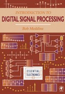
As an example, consider the simple discrete processing system shown in Fig. 2.13. As only the previous input samples are used, along with the current input, you will recognize this as an FIR or non-recursive filter. As the input and output sequences are represented by x[n] and y[n] respectively, and the time delay of one sample period is depicted by a ‘T’ box (where T is the sampling period), then this is obviously the time domain model. The processing being carried out is fairly simple, in that the input sequence, delayed by one sampling period and multiplied by a factor of −0.4, is added to the undelayed input sequence to generate the output sequence, y[n]. This can be expressed mathematically as:
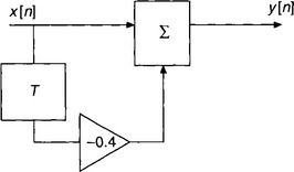
Figure 2.13
However, we have chosen to abandon the time domain and work in the z-domain and so the first thing we will need to do is convert our processing system of Fig. 2.13 to its z-domain version. This is shown in Fig. 2.14.

Figure 2.14
This is a very simple conversion to carry out. The input and output sequences, x[n] and y[n], of Fig. 2.13, have just been replaced by their z-transforms, and the time delay of T is now represented by z–1, the usual way of indicating a time delay of one sampling period in the z-domain.
The mathematical representation of the ‘z-domain’ processor now becomes:
or

i.e. we can find the transfer function of the processor quite easily. Armed with this we should be able to predict the response of the system to any input, either manually, or with the help of MATLAB.
N.B. The z-domain transfer function could also have been found by just converting equation (2.1) to its z-domain equivalent, i.e. Y(z) = X(z) − 0.4X(z)z–1, and so on (X(z)z–1 represents the input sequence, delayed by one sampling period).
2.14 FIR FILTERS AND THE z-DOMAIN
The processor we have just looked at is a simple form of a finite impulse response, or non-recursive filter. The z-domain model of a general FIR filter is shown in Fig. 2.15.

Figure 2.15
Each z–1 box indicates a further delay of one sampling period. For example, the input to the amplifier a3 has been delayed by three sample periods and so the signal leaving the amplifier can be represented by a3X(z)z–3.
The processor output is the sum of the input sequence and the various delayed sequences and is given by:
and so:
2.15 IIR FILTERS AND THE z-DOMAIN
These, of course, are characterized by a feedback loop. Weighted versions of delayed inputs and outputs are added to the input sample to generate the current output sample. Figure 2.16 shows the z-domain model of a simple example of this type of filter which adds only previous outputs to the current input.

Figure 2.16
Example 2.8
What is the transfer function of the IIR filter shown in Fig. 2.16?
Solution: This one is slightly more difficult to derive than that for the FIR filter. However, as before, we first need to find Y(z).
From Fig. 2.16:

Figure 2.17 shows a more general IIR filter, making use of both the previous outputs and inputs. This arrangement provides greater versatility.

Figure 2.17
It shouldn’t be too difficult to show that the transfer function for this general recursive filter is given by:
Try it!
Reminder
• Recursive (IIR) filters can be used to achieve the same processing as almost all non-recursive (FIR) filters but have the advantage of needing fewer multipliers/coefficients and so are simpler in terms of hardware.
• As with any system that uses feedback, a recursive filter can be unstable – this is not the case with FIR filters – these are always stable. (We will find later that IIR filters also have a ‘phase problem’ compared to FIR filters.)
Example 2.9
An FIR filter has three coefficients, a0 = 0.5, a1 = −0.8 and a2 = 0.4. Derive the output sequence corresponding to the finite input sequence of 1, 5.
Solution: We could derive this from first principles, by first drawing the z-domain diagram. However, by inspection of the transfer function for an FIR filter given earlier (equation (2.2)):
Also, as x[n] = 1, 5:

which gives:
So the output sequence is 0.5, 1.7, −3.6, 2.
The MATLAB output display is shown in Fig. 2.18.

Figure 2.18
Example 2.10
A filter has a transfer function given by
(a) Draw the z-domain version of the block diagram for the filter.
(b) Derive an expression for the output sequence y[n], in terms of the input sequence, x[n], and delayed input and output sequences.
(c) Find the unit sample response for the filter (first four terms only).
(a) This is clearly a recursive filter. By comparison with the general expression given earlier (equation (2.3)), this filter has coefficients of a0 = 1, a1 = −0.4, b1 = 0, b2 = −0.2 and so the z-domain block diagram is as shown in Fig. 2.19.

Figure 2.19
N.B. The two ‘z–1’ boxes, used to feed back the output sequence, could be replaced by a single ‘z–2’ box.

Carrying out the polynomial division gives T(z) = 1 − 0.4z–1 − 0.2z–2, to three terms. Check this for yourself – note that you will need to divide 1 − 0.4z–1 by 1 + 0z–1 + 0.2z–2.
As the z-transform of the input is just ‘1’, the z-transform of the output sequence will be exactly the same as the transfer function, i.e. Y(z) = 1 − 0.4z–1 − 0.2z–2 and so the first three terms of the output sequence will be 1, −0.4, −0.2.
The MATLAB output display is shown in Fig. 2.20.
Figure 2.20
N.B. The sampled output signal is shown in Fig. 2.20 as pulses, rather than ‘steps’. This improved display is achieved by using the MATLAB ‘stem’ function. The program is as follows:

2.16 SELF-ASSESSMENT TEST
1. Derive the transfer function for the IIR filter shown in Fig. 2.21 and, hence, find the first three terms of its unit sample response.

Figure 2.21
2. A simple running average filter generates the average of the current and previous input samples. Draw the ‘z-domain’ block diagram of the system. Hence, derive the transfer function of the filter and use it to find the response to an input of a discrete unit ramp (first three terms only). (Y(z) = z–1 + 2z–2 + 3z–3 + … for a unit ramp.)
3. A running average filter averages the current input and the previous five inputs. Show how this system could be realized with a recursive filter.
Hint: Find expressions for the output Y(z) and also the output delayed by one sample period, i.e. Y(z)z–1 – and then think about it!
4. Figure 2.22 is the z-domain block diagram for a biquadratic filter. Show that its transfer function, T(z), is given by:

Figure 2.22
Hint: Find two simultaneous equations by deriving expressions for V(z) and Y(z).
2.17 RECAP
• A non-recursive filter is one that makes use only of the current input sample and previous input samples. It is also called a finite impulse response filter (FIR) as it generates a finite output sequence in response to a finite input sequence. It has a general transfer function of: T(z) = a0 + a1z–1 + a2z–2 + a3z–3 + ….
• A recursive filter is one that has a feedback loop, i.e. it makes use of previous output values. It is also called an infinite impulse response filter (IIR) as, usually, it generates an infinite output sequence in response to a finite input sequence. If it combines the current input sample with only previous outputs then it has a general transfer function of
If it also makes use of previous inputs, as is most common, then it has the general transfer function of
• An IIR filter will require fewer coefficients/multipliers than the equivalent FIR filter.
2.18 CHAPTER SUMMARY
In this chapter we have looked at ways of representing discrete signals, both in the time domain and the z-domain. For example, a signal represented by x[n] = 1, 4, 6, 2 in the time domain can be expressed as X(z) = 1 + 4z–1 + 6z–2 + 2z–3 in the z-domain. Entering the z-domain allows us to analyse and design digital systems much more easily than working in the time domain.
The z-transform is used to move from the time domain to the z-domain. The z-transform of a sequence x[n] is given by
or x[0]z0 + x[1]z–1 + x[2]z–2 + x[3]z–3 + …. The ‘z–n’ operator can be thought of as a tag which indicates a delay of n sample periods.
The transfer function of a system in the z-domain is given by T(z) = Y(z)/X(z), where X(z) and Y(z) are the z-transforms of the input and output sequences respectively. The transfer function is used to find the system response to an input signal.
FIR and IIR filters have been revisited, but this time in the z-domain. FIR filters use the current input sample plus weighted previous inputs to generate the output, while IIR filters use weighted previous outputs as well.
The software package, MATLAB, has been used to analyse discrete systems.
2.19 PROBLEMS
1. An FIR filter has a transfer function of 1 + z–1. Find the output sequence in response to an input sequence of 1, 2, −2.
2. When the finite sequence 1, −3 is fed into an FIR filter, the output sequence is finite, and equal to 1, −2, −1, −6. Find the transfer function of the filter in the z-domain and also the response of the filter to a discrete unit step (first four terms only).
3. The output sequence, y[n], from a recursive filter, is related to its input sequence, x[n], as: y[n] = x[n] + 0.5x[n–1] + 0.5y[n–1]. Draw the block diagram for this filter, in the z-domain, and find its transfer function. Use the transfer function to find the filter’s response to a unit sample sequence (first four terms only).
4. A filter has a transfer function of T(z) = (z + 1)(z − 1)/z2. Find its response to the finite sequence 1, 0, 2 (first five terms only).
5. Find the transfer function for the processor shown in Fig. 2.23.

Figure 2.23
6. Use z-transform tables to find the response of a digital filter to a discrete unit step, given that the filter has the transfer function of 0.8/(z − 0.2). Only the first four terms are required.