The basics
1.1 CHAPTER PREVIEW
In this first chapter you will be introduced to the basic principles of digital signal processing (DSP). We will look at how digital signal processing differs from the more conventional analogue signal processing and also at its many advantages. Some simple digital processing systems will be described and analysed. The main aim of this chapter is to set the scene and give a feel for what digital signal processing is all about – most of the topics mentioned will be revisited, and dealt with in more detail, in other chapters.
1.2 ANALOGUE SIGNAL PROCESSING
You are probably very familiar with analogue signal processing. Some obvious examples of this type of processing are amplification, rectification and filtering. With all analogue processing, signals enter a system, are processed by passing them through circuits containing capacitors, resistors, inductors, op amps, transistors etc. They are then outputted from the system with a different shape or size. Figure 1.1 shows a very elementary example of an analogue signal processing system, consisting of just a resistor and a capacitor – you will probably recognize it as a simple type of lowpass filter. Analogue signal processing circuits are commonplace and have been very important system building blocks since the early days of electrical engineering.

Figure 1.1
Unfortunately, as useful as they are, analogue processing systems do have major defects. An obvious one is that they have to be physically modified if the processing needs to be changed. For example, if the gain of an amplifier has to be increased, then this usually means that at least a resistor has to be changed. What if a different cut-off frequency is required for a filter or, even worse, we want to replace a highpass filter with a lowpass filter? Once again, components must be changed. This can be very inconvenient to say the least – it’s bad enough when a single system has to be adjusted but imagine the situation where a batch of several thousand is found to need modifying. How much better if changes could be achieved by altering a parameter or two in a computer program …
Another problem with analogue systems is that of ‘repeatability’. It is very unlikely that two analogue systems will have identical performances, even though they have been made in exactly the same way, with supposedly the same value components. This is mainly because of component tolerances. Analogue devices have two further disadvantages. The first is that their components age and so the device performance changes. The other is that components are also affected by temperature changes.
1.3 AN ALTERNATIVE APPROACH
So, having slightly dented the reputation of analogue processors, what’s the alternative? Luckily, signal processing systems do exist which work in a completely different way and do not have these problems. A major difference is that these systems first sample, at regular intervals, the signal to be processed (Fig. 1.2). The sampled voltages are then converted to equivalent binary values, using an analogue-to-digital converter (Fig. 1.3). Next, these binary numbers are fed into a digital processor, containing a particular program, which will change the samples. The way in which the digital values are modified will obviously depend on the type of signal processing required – for example, do we want lowpass or highpass filtering and what cut-off frequency do we require? The transformed samples are then outputted, via a digital-to-analogue converter, to produce the reconstituted but processed analogue output signal.
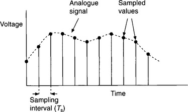
Figure 1.2

Figure 1.3
Because computers can process data so quickly, the signal processing can be done almost in ‘real time’, i.e. the processed output samples are fed out continuously, almost in step with the corresponding input samples. Alternatively, the processed data could be stored, perhaps on a chip or CD-ROM, and then read when required.
By now, you’ve probably guessed that this form of processing is called digital signal processing. Digital signal processing (DSP) does not have the drawbacks of analogue signal processing, already mentioned. For example, the type of processing required can be modified very easily – if the specification of a filter needs to be changed then new parameters can simply be keyed into the DSP system, i.e. the processing is programmable. The performance of a digital filter is also constant, not changing with either time or temperature. DSP systems are also inherently repeatable – if several DSP systems have been programmed to process signals in a certain way then they will all behave identically. DSP systems can also process signals in ways impossible for analogue systems.
• Digital signal processing systems are available that will do almost everything that analogue signals can do, and much more – ‘versatile’.
• They can be easily changed – ‘programmable’.
• They can be made to process signals identically – ‘repeatable’.
• They are not affected by temperature or ageing – ‘physically stable’.
1.4 THE COMPLETE DSP SYSTEM
The heart of the digital signal processing system, the analogue-to-digital converter (ADC), digital processor and the digital-to-analogue converter (DAC), is shown in Fig. 1.3. However, this sub-unit needs ‘topping and tailing’ in order to create the complete system. An entire, general DSP system is shown in Fig. 1.4.
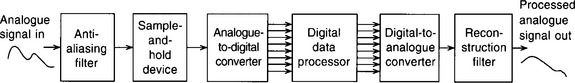
Figure 1.4
Each block will now be described briefly.
The anti-aliasing filter
If the analogue input voltage is not sampled frequently enough then this results in something of a shambles. Basically, high frequency input signals will appear as low frequency signals at the output, which will be very confusing to say the least! This phenomenon is called aliasing. In other words, the high frequency input signals take on another identity, or ‘alias’, on leaving the system.
To get a feel for the problem of aliasing, consider a sinusoidal signal, of fixed frequency, which is being sampled every 7/8 of a period, i.e. 7T/8 (Fig. 1.5). Having only the samples as a guide, it can be seen that the sampled signal appears to have a much lower frequency than it really has.
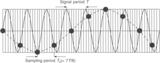
Figure 1.5
In practice, a signal will not usually have a single frequency but will consist of a very wide range of frequencies. For example, audio signals can contain frequency components in the range of about 20 Hz to 20 kHz.
To prevent aliasing, it can be shown that the signal must be sampled at least twice as fast as the highest frequency component.
This very important rule is known as the Nyquist criterion, or Shannon’s sampling theorem, after two distinguished pioneers from the world of signal processing.
If this sampling rate cannot be achieved, perhaps because the components used just cannot respond this quickly, then a lowpass filter must be used on the input end of the system. This has the job of removing signal frequencies greater than fs/2, where fs is the sampling frequency. This is the role of the anti-aliasing filter. An anti-aliasing filter is therefore a lowpass filter with a cut-off frequency of fs/2.
The important frequency of fs/2 is usually called the Nyquist frequency.
The sample-and-hold device
An ADC should not be presented with a changing voltage to convert. The changing signal should be sampled and then this sampled voltage held while the conversion is carried out (Fig. 1.6). (In practice, the sampled value is normally held until the next sample is taken.) If the voltage is not kept constant during conversion then, depending on the type of converter used, the digital output might not just be a little inaccurate but could be absolute rubbish, bearing no relationship to the true value.

Figure 1.6
At the heart of the sample-and-hold device is a capacitor (Fig. 1.7). The electronic switch, S, is closed, causing the capacitor to charge to the current value of the input voltage. After a brief time interval the switch is reopened, so keeping the sampled voltage across the capacitor constant while the ADC carries out its conversion. The complete sample-and-hold device usually includes a voltage follower at both the input and the output of the basic system shown in Fig. 1.7. The characteristically low output impedance and high input impedance of the voltage followers ensure that the capacitor is charged very quickly by the input voltage and discharges very slowly through the ADC connected to its output, so maintaining the stored voltage.
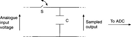
Figure 1.7
The analogue-to-digital converter
This converts the steady, sampled voltage, supplied by the sample-and-hold device, to an equivalent digital value in preparation for processing. The more output bits the converter has, the finer the resolution of the device, i.e. the smaller is the voltage change represented by the least significant output bit changing from 0 to 1 or from 1 to 0.
You are probably aware that there are many different types of ADC available. However, some of these are too slow for most DSP applications, e.g. single- and dual-slope and the basic counter-feedback versions. An ADC widely used in DSP systems is the sigma-delta converter. If you feel the need to do some extra reading in order to brush up on ADCs then some keywords to look out for are: single-slope, dual-slope, counter-feedback, successive approximation, flash, tracking and sigma-delta converters and also converter resolution. Millman and Grabel (1987) is just one of many books that give a good general treatment, while Marven and Ewers (1994) and also Proakis and Manolakis (1996) are two texts that give good coverage of the sigma-delta converter.
The processor
This could be a general-purpose microprocessor chip, but this is unlikely. The data processing part of a purpose-built DSP chip is designed to be able to do a limited number of fairly simple operations, in particular addition and multiplication, but they do these exceptionally quickly. Most of the major chip-producing companies have developed their own DSP chips, e.g. Motorola, Texas Instruments and Analog Devices, and their user manuals are obvious reference sources for further reading.
The digital-to-analogue converter
This converts the processed digital value back to an equivalent analogue voltage. Common types are the ‘weighted resistor’ and the ‘R-2R’ ladder converters, although the weighted resistor version is not a practical proposition, as it cannot be fabricated sufficiently accurately as an integrated circuit. Details of these two devices can be found in Millman and Grabel (1987), while Marven and Ewers (1994) describes the more sophisticated ‘bit-stream’ DAC, often used in DSP systems.
The reconstruction filter
As the anti-aliasing filter ensures that there are no frequency components greater than fs/2 entering the system, then it seems reasonable that the output signal will also have no frequency components greater than fs/2. However, this is not so! The output from the DAC will be ‘steppy’ because the DAC can only output certain voltage values. For example, an 8-bit DAC will have 256 different output voltage levels going from perhaps −5 V to +5 V. When this quantized output is analysed, frequency components of fs, 2fs, 3fs, 4fs etc. (harmonics of the sampling frequency) are found. The very action of sampling and converting introduces these harmonics of the sampling frequency into the output signal. It is these harmonics which give the output signal its steppy appearance. The reconstruction filter is a lowpass filter having a cut-off frequency of fs/2, and is used to filter out these harmonics and so smooth the output signal.
1.5 RECAP
• Analogue signal processing systems have a variety of disadvantages, such as components needing to be changed in order to change the processor function, inaccuracies due to component ageing and temperature changes, processors built in the same way not performing identically.
• Digital processing systems do not suffer from the problems above.
• Digital signal processing systems sample the input signal and convert the samples to equivalent digital values. These values are processed and the resulting digital outputs converted back to analogue voltages. This series of discrete voltages is then smoothed to produce the processed analogue output.
• The analogue input signal must be sampled at a frequency which is at least twice as high as its highest frequency component, otherwise ‘aliasing’ will take place.
1.6 DIGITAL DATA PROCESSING
For the rest of this chapter we will concentrate on the processing of the digital values by the digital data processing unit – this is where the clever bit is done!
So, how does it all work? The digital data processor (Fig. 1.4) is constantly being bombarded with digital values, one following the other at regular intervals. Its job is to output a suitable digital number in response to each digital input. This is something of an achievement as all that the processor has to work with is the current input value and the previous input and output samples. Somehow it has to use these to generate the output value corresponding to the current input value.
The mechanics of what happens is surprisingly simple. First, a number of the previous input and/or output values are stored in special data storage registers, the number stored depending on the nature of the signal processing to be done. Weighted versions of these stored values are then added to (or subtracted from) the current input sample to generate the corresponding output value – the actual algorithm obviously depending on the type of signal processing required. It is this processing algorithm which is at the heart of the whole system – arriving at this can be a very complicated business! This is something we will examine in detail in later chapters. Here we will look at some fairly simple examples of processing, just to get a feel for what is involved.
1.7 THE RUNNING AVERAGE FILTER
A good example to start with is the running (or moving) average filter. This processing system merely outputs a value which is the average of the current input and a particular number of the previous input samples.
As an example, consider a simple running average filter that averages the current input and the last three input samples. Let’s assume that the sampled input values are as shown in Table 1.1, where T represents the sampling period.
Table 1.1
| Time | Input sample |
| 0 | 2 |
| T | 1 |
| 2T | 4 |
| 3T | 5 |
| 4T | 7 |
| 5T | 10 |
| 6T | 8 |
| 7T | 7 |
| 8T | 4 |
| 9T | 2 |
As we need to average the current sample and the previous three input samples, the processor will clearly need three registers to store the previous input samples, the contents of these registers being updated every time a new sample is taken. For simplicity, we will assume that these three registers have initially been reset, i.e. they contain the value zero.
The following sequence shows how the first three samples of ‘2’, ‘1’, and ‘4’ are processed:

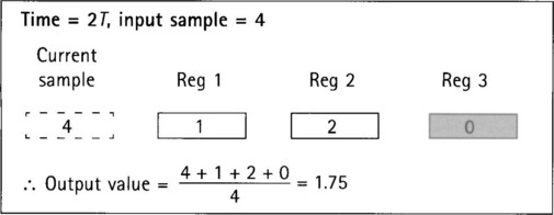
Table 1.2 shows all of the output values – check that you agree with them before moving on.
Table 1.2
| Time | Input sample | Output sample |
| 0 | 2 | 0.5 |
| T | 1 | 0.75 |
| 2T | 4 | 1.75 |
| 3T | 5 | 3.00 |
| 4T | 7 | 4.25 |
| 5T | 10 | 6.50 |
| 6T | 8 | 7.50 |
| 7T | 7 | 8.00 |
| 8T | 4 | 7.25 |
| 9T | 2 | 5.25 |
N.B.1. The first three output values of 0.5, 0.75 and 1.75, represent the initial ‘transient’, i.e. the part of the output signal where the initial three zeros are being shifted out of the three storage registers. The output values are only valid once these initial zeros have been cleared out of the storage registers.
N.B.2. A running average filter tends to smooth out any rapid changes in a signal and so is a form of lowpass filter.
1.8 REPRESENTATION OF PROCESSING SYSTEMS
The running average filter, just discussed, could be represented by the block diagram shown in Fig. 1.8. Each of the three ‘T’ blocks represent a time delay of one sample period, while the ‘Σ’ box represents the summation of the four values. The ‘0.25’ triangle is an attenuator which ensures that the average of the four values is outputted and not just the sum. So A is the current input divided by four, B the previous input, again divided by four, C the input before that, again divided by four etc. If we catch the system at 6T say, then, from Table 1.2, A = 8/4, B = 10/4, C = 7/4 and D = 5/4, giving the output of 7.5, i.e. A + B + C + D.

Figure 1.8
N.B. The division by four could have been done after the summation rather than before, and this might seem the obvious thing to do. However, the option used is preferable as it means that, as we are processing smaller numbers, i.e. numbers already divided by four, we can get away with using smaller registers during processing. Here there were only four numbers to be added, but what if there had been a thousand? Dividing before addition, rather than after, would clearly makes a huge difference to the size of the registers needed.
1.9 SELF-ASSESSMENT TEST
Calculate the corresponding output samples if the sampled signal, shown in Fig. 1.9, is passed through a running average filter. The filter averages the current input sample and the previous two samples. Assume that the two processor storage registers needed are initially reset, i.e. contain the value zero. (The worked solution is given towards the end of the book.)

Figure 1.9
1.10 FEEDBACK (OR RECURSIVE) FILTERS
So far we have only met filters which make use of previous inputs. There is nothing to stop us from using the previous outputs instead – in fact, much more useful filters can be made in this way. A simple example is shown in Fig. 1.10.

Figure 1.10
Because it is the previous output values which are fed back into the system and added to the current input, these filters are called feedback or recursive filters. Another name very commonly used is infinite impulse response filters – the reason for this particular name will become clear later.
As we know, the T boxes represent time delays of one sampling period, and so A is the previous output and B the one before that. It is often useful to think of these boxes as the storage registers for the previous outputs, with A and B being their contents.
From Fig. 1.10 you should see that:
This is the simple processing that the digital processor needs to do for every input sample.
Imagine that this particular recursive filter is supplied with the data shown in Table 1.3, and that the two storage registers needed are initially reset.
Table 1.3

From equation (1.1), as both A and B are initially zero, the first output must be the same as the input value, i.e. ‘10’.
By the time the second input of 15 is received the previous output of 10 has been shifted into the storage register, appearing as ‘A’ (Table 1.3). In the meantime, the previous A value (0) has been moved to B, while the previous value of B has been shifted right out of the system and lost, as it is no longer of any use.
So, when time = T, we have:Input data = 15, A = 10, B = 0
From equation (1.1), the new output value is given by:
In preparation for generating the next output value, the current output of 11 is now shifted to A, the A value of 10 having already been moved to B. The third output value is therefore given by:
20 − 0.4 × 11 + 0.2 × 10 = 17.6
Before moving on it’s best to check through the rest of Table 1.3 for yourself. (Spreadsheets lend themselves well to this application.)
You will notice from Table 1.3 that we are getting outputs even when the input values are zero (at times 7T, 8T and 9T). This makes sense as, at time 7T, we are pushing the previous output value of 8.5 back through the system to produce the next output of −2.4. This output value is, in turn, fed back into the system, and so on. Theoretically, the output could continue for ever, i.e. even if we put just a single pulse into the system we could get output values, every sampling period, for an infinite time. This explains the alternative name of infinite impulse response (IIR) filter for feedback filters. Note that this persisting output will not happen with processing systems which use only the input samples (‘non-recursive’) – with these, once the input stops, the output will continue for only a finite time. To be more specific, the output samples will continue for a time of N × T, where N is the number of storage registers. This is why filters which make use of only the previous inputs are often called finite impulse response (FIR) filters (pronounced ‘F-I-R’), for short. A running average filter is therefore an example of an FIR filter. (Yet another name used for this type of filter is the transversal filter.)
IIR filters require fewer storage registers than equivalent FIR filters. For example, a particular highpass FIR filter might need 100 registers but an equivalent IIR filter might need as few as three or four. However, I must add a few words of warning here, as there are drawbacks to making use of the previous outputs. As with any system which uses feedback, we have to be very careful during the design as it is possible for the filter to become unstable. In other words, instead of acting as a well-behaved system, processing our signals in the required way, we might find that the output values very rapidly shoot up to the maximum possible and sit there. Another possibility is that the output oscillates between the maximum and minimum values. Not a pretty sight! We will look at this problem in more detail in later chapters.
So far we have looked at systems which make use of either previous inputs or previous outputs only. This restriction is rather artificial as, generally, the most effective DSP systems use both previous inputs and previous outputs.
1.11 SELF-ASSESSMENT TEST
As has just been mentioned, DSP systems often make use of previous inputs and previous outputs. Figure 1.11 represents such a system.
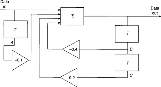
Figure 1.11
(a) Derive the equation which describes the processing performed by the system, i.e. relates the output value to the corresponding input value.
(b) If the input sequence is 3, 5, 6, 6, 8, 10, 0, 0 determine the corresponding output values. Assume that the three storage registers needed (one for the previous input and two for the previous outputs) are initially reset, i.e. contain the value zero.
1.12 CHAPTER SUMMARY
Hopefully, you now have a reasonable understanding of the basics of digital signal processing. You should also realize that this type of signal processing is achieved in a very different way from ‘traditional’ analogue signal processing. In this chapter we have concentrated on the heart of the DSP system, i.e. the part that processes the digital samples of the original analogue signal. Several processing systems have been analysed. At this stage it will not be clear how these systems are designed to achieve a particular type of signal processing, or even the nature of the signal processing being carried out. This very important aspect will be dealt with in more detail in later chapters. We have met finite impulse response filters (those that make use of previous input samples only, such as running average filters) and also infinite impulse response filters (also called feedback or recursive filters) – these make use of the previous output samples. Although ‘IIR’ systems generally need fewer storage registers than equivalent ‘FIR’ systems, IIR systems can be unstable if not designed correctly, while FIR systems will never be unstable.
1.13 PROBLEMS
1. Describe, briefly, four problems associated with analogue signal processing systems but not with digital signal processing systems.
2. ‘An FIR filter generally needs more storage registers than an equivalent IIR filter.’ True or false?
3. A running average filter has a frequency response which is similar to that of:
4. What are two alternative names for IIR filters?
5. ‘Once an input has been received, the output from a running average filter can, theoretically, continue for ever.’ True or false?
6. ‘An FIR filter can be unstable if not designed correctly.’ True or false?
7. A signal is sampled for 4 s by an 8-bit ADC at a sampling frequency of 10 kHz. The samples are stored on a memory chip.
(a) What is the minimum memory required to store all of the samples?
(b) What should be the highest frequency component of the signal?
8. If the sequence 3, 5, 7, 6, 3, 2 enters the processor shown in Fig. 1.12, find the corresponding outputs.

Figure 1.12
9. The sequence 2, 3, 5, 4 is inputted to the processing system of Fig. 1.13. Find the first six outputs.

Figure 1.13
10. A single input sample of ‘1’, enters the system of Fig. 1.14. Find the first eight output values. Is there something slightly worrying about this system?
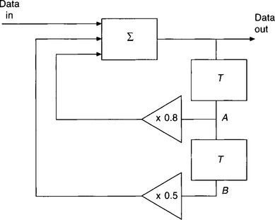
Figure 1.14