
Answers to self-assessment tests and problems
Chapter 1
As this is a running average filter which averages the current and previous two input samples, then:
Applying this equation, and remembering that the two storage registers are initially reset, the corresponding input and output values will be as shown in Table S1.1. The first two output values of 0.67 and 1.67 are not strictly valid as the two zeros, initially stored in the two storage registers, are still feeding through the system.
Table S1.1
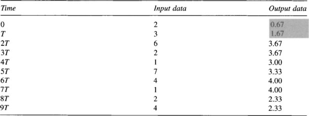
The input and output values are also shown in Fig. S1.1. Notice how the averaging tends to smooth out the variations of the input signal. This is a good demonstration that the running average filter is a type of lowpass filter.

Figure S1.1
Section 1.11
(a) From Fig. 1.11:
(b) Table S1.2 shows all outputs, and also the A, B and C values, corresponding to the eight input samples.
Table S1.2

Problems
(b) Unlikely that two ‘identical’ analogue processors will behave in an identical way.
5. False (true for IIR filters – running average is an FIR filter).
6. False (only true for IIR filters).
8. 3, 4.4, 6.9, 6.1, 3.9, 3.2.
9. 2.00, 2.60, 4.56, 3.18, −0.47, 0.19.
10. 1, 1, 1.2, 1.4, 1.64, 1.92.
It looks suspiciously as though the output will continue to increase with time, i.e. that the system is unstable. (In fact, this particular system is unstable and needs redesigning.)
Chapter 2
To avoid aliasing, this signal must be sampled at a minimum of 3 Hz, and so 20 Hz is fine.
(b) As the sampling frequency is 20 Hz, the samples are the signal values at 0, 0.05, 0.1, 0.15, 0.2 and 0.25 s.
(c) x[n − 4] = 0, 0, 0, 0, 2, 1.78, 1.17, 0.31, −0.62, −1.42.
(a) From Fig. 2.8, the sequence at A is −2(x[n − 1]) = 0, −4, −2, −6, 2.


Section 2.16
Dividing (1 − 0.8z−1) by (1 − 0.5z−1) you should get 1 − 0.3z−1 − 0.15z−2 … and so the first three terms of the output sequence are 1, −0.3 and −0.15.
2. From Fig. S2.1:
As the z-transform for a unit ramp is 0 + z−1 + 2z−2 + 3z−3 + …, then the z-transform of the system output is given by:
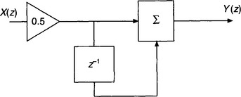
Figure S2.1
Equation (S2.2) – equation (S2.1):

i.e. this is the transfer function for a recursive filter.


Problems
2. T(z) = 1 + z−1 + 2z−2. Unit step response: 1, 2, 4, 4.
3. T(z) = (1 + 0.5z−1)/(1 − 0.5z−1) = 1 + z−1 + 0.5z−2 + 0.25z−3.
Unit sample response: 1, 1, 0.5, 0.25.
4. Output sequence: 1, 0, 1, 0, −2. [T(z) = (1 − z−2)].
5. T(z) = 0.5(1 − 0.4z−1)/(l − z−2). (Hint: The input to the ×0.5 attenuator is 2Y(z).)
Chapter 3
There is therefore a single zero at s = −2. There is a pole at s = 0 and also at s = −3 and −1 (roots of s2 + 4s + 3). The pole–zero diagram is shown in Fig. S3.1. The pole at A will correspond to a step of height k1, while the poles at B and C represent exponentially decaying d.c. signals of k2e−t and k3e−3t respectively, where k1, k2 and k3 are multipliers. (Although it is possible to find the k-values from the p–z diagram, this is not expected here.) Figure S3.2 shows the MATLAB plots for the signals corresponding to the three pole positions (k-values of 1 have been used for all three signals, as it is only general signal shapes that are required).
which gives a = 4/3, b = −1 and c = −1/3. Therefore, from the Laplace transform tables:
2. This transform has no zeros but has poles at s = ± j2 and so this represents a non-decaying sine wave of angular frequency 2. From the Laplace transform tables:

Figure S3.1

Figure S3.2
i.e. the transform first needs to be rearranged to 3 × 2/(s2 + 22). It can then be recognized as a standard transform.
Section 3.11
1. This p–z diagram represents an exponentially decaying d.c. signal – the signal samples falling to 0.8 of the previous sample – the pulse train being delayed by one sampling period. Carrying out the polynomial division, i.e. dividing z−1 by 1 − 0.8z−1, results in the series z−1 + 0.8z−2 + 0.64z−3 + … (N.B. This assumes no ‘pure’ gain in the system, i.e. that T(z) = k/(z − 0.8) where k = 1. It is impossible to know the true value of k from the p–z diagram alone.)
2. The Nyquist frequency (fN) = 60 Hz, i.e. 180° = 60 Hz.
Pole-pair B1 and B2:
This represents conjugate poles 0.61 from the origin, the pole vectors to the origin being inclined at angles of ±0.5 radians from the positive real axis.
i.e. the pole vectors have a magnitude of 1 and are inclined at ±0.5 radians (±28.6°) to the positive real axis.
The z-plane p–z diagram is shown in Fig. S3.3.

Figure S3.3
Section 3.15
Therefore there are real s-plane zeros at s = −1 and −2 and complex conjugate poles at −1 ±j (roots of the denominator). Figure S3.4 shows the p–z diagram.

Figure S3.4

1 rad/s (Point B,Fig. S3.5):
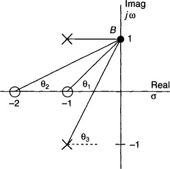
Figure S3.5

A similar approach should show that the gain and phase angle at 2 rad/s are 5.66 (15 dB) and −8.2°.
For very large frequencies the distances from the frequency point to the two poles and the two zeros are almost identical and so the gain must be very close to 4. Further, as the angles made by the zero and pole vectors approach 90° then the phase angle must be zero. Figure S3.6 shows the Bode plot for the system.

Figure S3.6
Section 3.18
One zero at z = 0 and three poles at z = 0.8 and −0.5 ± j0.5.
The p–z diagram is shown in Fig. S3.7.

Figure S3.7
As the Nyquist frequency is 8 Hz, points A and B must represent signal frequencies of 0 and 4 Hz respectively.
and
it should be fairly easy to show that the magnitude and phase angle of the frequency response at 0 Hz are 2 and 0° respectively.
From Fig. S3.7:


Problems
(a) Zero at 0.1 and pole at 0.3.
(b) Gain at 0 Hz = 1.29, phase angle = 0.
(b) The d.c. gains of the continuous and digital filters are approximately 0.67 and 7.36 respectively. It follows that the transfer function of the digital filter would have to be scaled by multiplying by 0.67/7.36.
(a) As the z-transform for the unit sample function is 1, then
i.e. no zeros but poles at 0.5 ± j0.5.
(b) The z-transform of a unit step is z/(z − 1). It follows that
i.e. p–z diagram as for (a) above, but an extra pole at +1 and a zero at the origin. Gain at 0 Hz = 2 and at fs/4 = 0.89.
4. Dividing z2 by z + 1 (or z by 1 + z−1) results in the z-transform of z − 1 + z−1 − z−2 + … for the unit sample response. The initial z indicates that the output sequence begins one sampling period before the input arrives! Impossible!
The gain at 0 Hz is approximately 1.2.
The filter is a bandstop filter, with maximum gains of 1.2 at 0 and 100 Hz (fN) and minimum gain of 0.5 (−6 dB) at 50 Hz.
Chapter 4
There must therefore be two poles at z = ± ja.Figure S4.1 shows the two poles and also points A, B and C corresponding to signal frequencies of 100, 90 and 110 Hz respectively. (N.B. The positions of points B and C on the unit circle are not drawn to scale.)
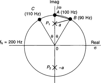
Figure S4.1
At 100 Hz (Point A):
(‘(1 + a)’ as B is very close to A)
As the angle ∠AOB is relatively small (≈9°), arc AB ≈ line AB. Also, triangle P1AB approximates to a right-angled triangle, with ∠P1AB ≈ 90°.

Dividing equation (S4.2) by (S4.1), and carrying out a few lines of algebra, you should eventually find that a ≈ 0.86. Substituting this value back into equation (S4.1) or (S4.2) should give k ≈ 0.26.
Section 4.9
First check whether pre-warping is necessary:

This is approximately a 5% difference compared to ωc, and so pre-warping is necessary.
Replacing all s/ωc terms with ![]() :
:
Applying the bilinear transform:

After a few lines of algebra:
Section 4.11
From the s/z transform tables:
Scaling the z-domain transfer function so that the d.c. gains of the two filters become the same:

Applying the method of partial fractions:
Using the ‘cover-up’ rule (or any other method):
From the s/z transform tables:
After a few lines of algebra, you should find that
and, after equalizing the d.c. gains of the two filters:
Section 4.13
This particular continuous filter has no zeros and a double pole at s = −2.
From z = esT, the equivalent pole positions in the z-plane must be given by z = e−0.2 = 0.82.
(A double zero has been added at z = −1 to balance up the number of poles and zeros.)
After equalizing the d.c. gains of the filters, the final transfer function is given by:
i.e. a zero at s = −2 and two poles at s = −1 and −3. These transform to a zero in the z-plane at z = 0.819 and poles at 0.905 and 0.741.
or
after scaling.

Chapter 5
From Section 5.6:
Substituting n = −5 to +5 into equation (S5.1) gives coefficients of:

(b) The Hanning window function is given by:
Substituting n = 0 to 10 into equation (S5.2) gives Flanning coefficients of:
Multiplying the filter coefficients of part (a) by the corresponding Hanning coefficient gives a modified filter transfer function of:
or, more sensibly:
2. The filter coefficients are the same as those for the lowpass filter designed in Section 5.6, before applying the Hamming window function, apart from (a) the signs being changed and (b) the central coefficient being 1 − (fc/fN) = 0.6 (see Section 5.8).
Section 5.13
The required magnitude response and the sampled frequencies are shown in Fig. S5.1. From Section 5.12, equation (5.8b), the filter coefficients, x[n], are given by:
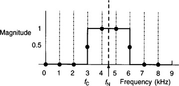
Figure S5.1
where N is the number of frequency samples taken (nine here), α = (N − 1)/2, i.e. 4, and |Xk| is the magnitude of the kth frequency sample. In this example |X0|, |X1| and |X2| = 0, while |X3| = 0.5 and |X4| = 1. Substituting into equation (S5.3)
Similarly, x[2] = 0.114677, x[3] = −0.264376 and x[4] = 0.333333

Problems


3. Magnitude and phase angle of the three frequency components of 0, 500 Hz and 1500 Hz are 3∠0°, 1.732∠90° and 1.732∠−90° respectively.


6. The FFT values are: 2, 1 − j3, 0, 1 + j3, i.e. the magnitudes of the four frequency components, 0, fs/4, fs/2 and 3fs/4 are 2, √10, 0 and √10 respectively, while the corresponding phase angles are 0, tan−1(−3), 0, tan−1 3.