
The design of FIR filters
5.1 CHAPTER PREVIEW
This, the final chapter, begins by making a case for the use of FIR filters rather than IIR filters under certain conditions. We will then look at two standard methods used to design FIR filters – the ‘Fourier’ or ‘windowing’ method and the ‘frequency sampling’ method. These two design techniques rely heavily on various forms of the Fourier transform and the inverse Fourier transform, and so these topics will also be covered, including the ‘fast Fourier transform’ and its inverse.
5.2 INTRODUCTION
So far we have looked at various ways of designing IIR filters. Compared to FIR filters, IIR filters have the advantage that they need significantly fewer coefficients to produce a roughly equivalent filter. On the downside, they do have the disadvantage that they can be unstable if not designed properly, i.e. if any of the transfer function poles are outside the unit circle. However, with careful design this should not happen.
5.3 PHASE-LINEARITY AND FIR FILTERS
Imagine a continuous signal, let’s say a rectangular pulse, being passed through a filter. Also imagine that the transfer function of the filter is such that the gain is 1 for all frequencies. Such filters exist and are called ‘all-pass’ filters. It would seem reasonable that the pulse will pass through an all-pass filter undistorted. However, this is unlikely to be the case. This is because we have not taken into account the phase response of the filter. When the signal passes through a filter, the different frequencies making up the rectangular pulse will usually undergo different phase changes – effectively, signals of different frequencies are delayed by different times. It is as though, as a result of passing through the filter, signals are ‘unravelled’ and then put back together in a different way. This reconstruction results in distortion of the emerging signal.
An example of a continuous, all-pass filter is one with the transfer function T(s) = (s − 4)/(s + 4). (Note that this transfer function has a zero on the right-hand side of the s-plane. This is fine – it is only poles which will cause instability if placed here.) This particular filter will have a gain of 1 for all frequencies – this should be fairly obvious from its p–z diagram. Interpretation of the signal response is made slightly easier if we imagine that we have an inverting amplifier in series with the filter. The frequency response, Fig. 5.1, confirms that the gain of the combination is 1. Figure 5.2 shows the response of the filter to a rectangular pulse – the signal has clearly been changed. Notice that the distortion occurs particularly at the leading and falling edges of the pulse. This would be expected, as the edges correspond to sudden changes in the signal magnitude and rapid changes consist of a broad band of signal frequencies. Figure 5.3 shows the output when a unit impulse passes through the filter. Theoretically, a unit impulse is composed of an infinite range of frequencies and so it should suffer major distortion – and it certainly does (notice how its width has spread to approximately 1 s). In a similar way, discrete all-pass filters will also cause distortion. Figure 5.4 shows what happens to a sampled rectangular pulse, consisting of three unit pulses, passed through such a filter.

Figure 5.1

Figure 5.2
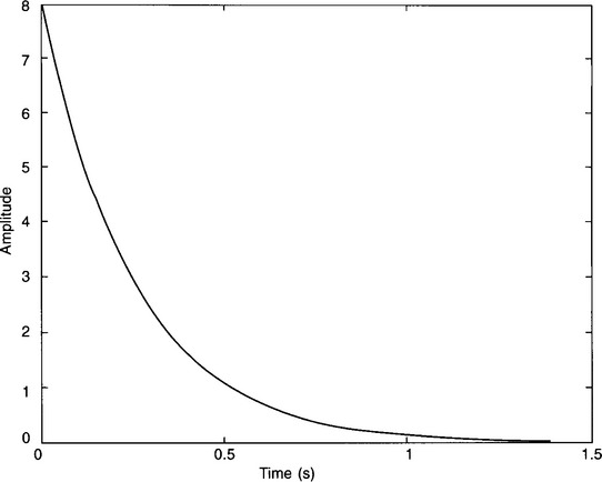
Figure 5.3

Figure 5.4
It can be shown that only if a filter is such that the gradient of the plot of phase shift against frequency is constant will there be no distortion of the signal due to the phase response.
This is because the effective signal delay introduced by a filter is given by dϕ/dω, where ϕ is the phase change. It follows that we require that ϕ = kω, where k is a constant, if the delay is to be the same for all frequencies, as then dϕ/dω = k.
Clearly, the phase response of our all-pass filter is not linear (Fig. 5.1), and so the signals suffer distortion. If a filter has a phase response with a constant gradient, i.e. where the phase response is linear then, very sensibly, the filter is described as being a ‘linear-phase filter’.
In the previous chapter we spent quite a lot of time converting continuous filters to their discrete IIR equivalents, and then comparing them very critically in terms of their magnitude responses. However, you might have noticed that not too much was made of any difference between their phase responses, even though the differences were sometimes very obvious. This is because the phase response of the original continuous filter itself was probably far from ideal and so it didn’t matter too much if the phase response of the discrete filter differed from it.
While we’re dealing with this subject, it should be mentioned that we can take an IIR filter with its poor, i.e. non-linear, phase response and place a suitable ‘all-pass’ discrete filter in series with it so as to linearize the combined phase responses. As well as having a gain of 1 for all signal frequencies, the compensating all-pass filter will have a phase response which is as close as possible to the inverse of that of the original filter.
So, to sum up, a case has been made for using FIR filters in preference to IIR filters, in certain circumstances. This is because FIR filters can be designed to have a linear phase response. As a result, such an FIR filter will not introduce any distortion into the output signal due to its phase characteristics. However, do not get the idea that all FIR filters are automatically linear-phase filters – far from it. If we want an FIR filter to have a linear phase response, and we usually do, then we need to design it to have this particular property.
5.4 RUNNING AVERAGE FILTERS
You met these filters way back in Chapter 1. Just to remind you, they are FIR filters that generate an output which is the average of the current input and a certain number of previous inputs. It is not a particularly useful filter practically – it behaves as a fairly ordinary lowpass filter. However, it is extremely useful to me at the moment in that it is an example of an FIR filter that naturally has a linear phase characteristic. For example, consider a running (or moving) average filter that averages the present and the previous three input samples, i.e.
where Y(z) and X(z) are the z-transforms of the filter output and input respectively.
or
Figure 5.5 shows the frequency response for this filter. Note that the magnitude response is that of a lowpass filter with a cut-off frequency of about 0.2fN but, much more importantly, that the phase response is linear. The discontinuity at 0.5fN doesn’t matter – what is important is that the gradient of the phase plot has a constant value.
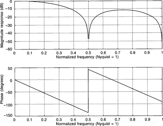
Figure 5.5
So, what is it about the transfer function of a running average filter that makes it a linear-phase filter?
The secret is the symmetry of the numerator coefficients. In this example all numerator coefficients are 1, and so definitely symmetric about the mid-point. However, any FIR filter with this central symmetry will exhibit a linear phase response. For example, if we had a filter with the transfer function:
or
i.e. symmetric coefficients of 2, 1, 3, 1, 2, then the phase response is as shown in Fig. 5.6 – i.e. once again a linear phase response, albeit split into segments.

Figure 5.6
So, to recap, when we design linear-phase FIR filters we must make sure that the coefficients of the transfer function numerator are symmetric about the centre, i.e. about the centre ‘space’ if there is an even number of coefficients and about the central coefficient if an odd number.
5.5 THE FOURIER TRANSFORM AND THE INVERSE FOURIER TRANSFORM
The first design method which we will use relies heavily on the Fourier transform, and so it makes sense to carry out a brief review of this extremely important topic at this point.
You are probably aware that the Fourier series allows us to express a periodic wave in terms of a d.c. value and a series of sinusoidal signals. The sinusoidal components have frequencies equal to the frequency of the original wave and harmonics of this ‘fundamental’ frequency. For example, a square wave consists of the fundamental frequency and weighted values of the odd harmonics. However, many signals are not periodic – speech would be an obvious example of a non-periodic waveform. This is where the Fourier transform is of such importance.
The Fourier transform, F(jω), of a signal, f(t), is defined by:
It is an extremely useful transform as it allows us to break a non-periodic signal, f(t), down into its frequency components, F(jω). F(jω) is normally complex, expressing both the magnitude and the phase of the frequency components. As the signal is non-periodic the component frequencies will cover a continuous band, unlike the discrete frequencies composing a periodic wave.
The inverse Fourier transform (IFT) allows us to work the other way round (the clue is in the name!). In other words, if we use the IFT to operate on the frequency spectrum of a signal, we can recover the time variation, i.e. the signal shape. The IFT is given by:

As it is the inverse Fourier transform which is more relevant to us in the design of FIR filters, it’s worth pausing here to look at an example of its use.
Let’s imagine that a signal has the spectrum of Fig. 5.7, i.e. it consists of frequencies in the range of –fc to +fc, all with equal weighting. As the Fourier transform of a signal is normally complex, it must be expressed in the form of an amplitude and a phase spectrum. For this particular signal we are assuming that the phase angle is zero for all frequencies, i.e. that its Fourier transform has no imaginary component. In other words, F(jω) = 1 for –fc ≤ f ≤ fc, else = 0.

Figure 5.7
N.B. You might not be familiar with the concept of ‘negative’ frequencies. Clearly, a negative frequency is meaningless practically. However, representing signals in terms of their ‘normal’ positive frequencies and also the equivalent negative frequencies is a neat mathematical ploy which helps with the analysis of the signals.
Applying the inverse Fourier transform (equation (5.1)) with F(jω) = 1:

N.B. We are now only integrating between −ωc and +ωc as F(jω) has a value of zero outside this frequency range.
but, from Euler’s identity,
This function is plotted in Fig. 5.8, using ωc = 5 rad/s and t = −10 s to +10 s. (There is nothing special about these values, they were chosen quite randomly.)

Figure 5.8
This signal might appear to be a little unusual and an unlikely one to meet on a regular basis! It is, in fact, an extremely important signal shape in the world of signal processing. Also, by using this simple frequency spectrum, the analysis was reasonably straightforward. You will find that this was a very useful example to have worked through when we move on to the design of an FIR in the next section.
So, to summarize, if we know the frequency spectrum of a signal we can use the IFT to derive the signal shape in the time domain. If we need to move in the opposite direction, i.e. from time domain to frequency domain, then we must use the Fourier transform.
This review is probably sufficient to allow us to move on but, if you feel that you need to do some more reading, there are plenty of circuit analysis/signal processing texts that deal with this topic. Some examples are: Howatson (1996), Denbigh (1998), Lynn and Fuerst (1994), Proakis and Manolakis (1996) and Meade and Dillon (1991). (Keywords: Fourier series, Fourier transform, inverse Fourier transform, amplitude spectrum, phase spectrum.)
5.6 THE DESIGN OF FIR FILTERS USING THE FOURIER TRANSFORM OR ‘WINDOWING’ METHOD
The starting point for this filter design method is the desired frequency response of the filter. To make use of the work done in the previous section, let’s suppose that we want to design an FIR lowpass filter with a cut-off frequency of 4 kHz. The required magnitude response is shown in Fig. 5.9. We will decide on the sampling frequency during the design process. We will assume that the phase response is zero, i.e. that signals of all frequencies experience no phase change on passing through the filter.
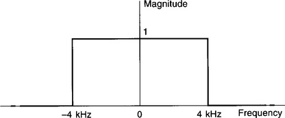
Figure 5.9
The first step in the design process is to move from the frequency domain to the time domain, by using the inverse Fourier transform. Luckily, we’ve already made this particular frequency-to-time conversion in the previous section (although for a frequency spectrum rather than a frequency response) and know that the corresponding time function, f(t), is given by:
Therefore, for this filter, with its cut-off frequency of 4 kHz:
But what exactly does this time function represent?
It is the unit impulse response of the filter. To convince yourself of this, you need to imagine using a unit impulse as the filter input. As the Laplace transform of the unit impulse is ‘1’, then the Laplace transform, Y(s), of the output, will be the same as the filter transfer function, i.e. Y(s) = 1 × T(s) = T(s). As we are interested in the frequency response, we can replace ‘s’ with jω. Therefore Y(jω) = T(jω), where Y(jω) is the frequency spectrum of the unit impulse response. We know that operating on the frequency spectrum of a signal with the IFT reconstructs the signal in the time domain. It follows that applying the IFT to T(jω), and therefore to Y(jω), must give us the time response of Y(jω), which we know is the unit impulse response of the filter. Make sure that you are happy with this argument, as it is fundamental to the design process.
Figure 5.10(a) shows the plot of f(t) = [sin (8000πt)]/πt, i.e. the filter unit impulse response, within the time window of −1.5 ms to +1.5 ms.

Figure 5.10
N.B. The time response shows a signal occurring before t = 0, i.e. before the input arrives, but don’t worry about this for the moment.
The next step in the design is to sample the unit impulse response. This is the crux of the design as these sampled values must be the FIR filter coefficients. For example, let’s imagine that we could represent the signal adequately by taking just five samples, a, b, c, b, a, with the samples being symmetric about the central peak. This, of course, is completely unrealistic and many samples would have to be taken – but bear with me.
If we now use these as the coefficients of the filter transfer function then this gives:
If we now use a unit sample sequence as the input to the discrete filter then the output will be the sequence a, b, c, b, a. It follows that the envelope of the unit sample response of the discrete filter will be the same as the unit impulse response of the continuous filter. In other words, we will have designed a digital filter that has the unit sample response which corresponds to the required frequency response.
This sounds fine, but we have a bit of a practical problem here in that the time response, theoretically, continues forever. Figure 5.10(a) shows only part of it; the ripples either side of the central peak gradually get smaller and smaller. Clearly we cannot take an infinite number of samples! What we have to do is compromise and sample over only a limited, but adequate, time span. Here we will sample between approximately ±5 × 10⁻⁴ s. This time slot is rather short but it will be adequate to demonstrate the principles of the approach. If we were to use a more realistic time window then the maths involved would become unnecessarily tedious and get in the way of the explanation.
If we wish one of our samples to be at the central peak, which seems a sensible thing to do, then, as the coefficients must be symmetric about the centre to ensure phase-linearity, it means that we will need to take an odd number of samples. Conveniently, if we sample every 0.5 × 10⁻⁴ s then we can fit exactly 21 samples into the 10−3 s time slot. We will therefore sample at 20 kHz (T = 0.5 × 10⁻⁴ s). This gives a Nyquist frequency of 10 kHz, which is well above the cut-off frequency of 4 kHz and so should be satisfactory. (Clearly, it would be pointless deciding to sample at a frequency that corresponds to a Nyquist frequency which is below the cut-off frequency!)
Before we carry out the sampling there is one other problem to address – that of the time response starting at a negative time. This has been referred to earlier but was put to one side. Clearly, this is an impossible response for a real digital filter as it means that a signal is generated before an input is received, in other words, the filter is ‘non-causal’. However, this not a major problem mathematically as we can just shift the required time response to the right by 0.5 × 10⁻³ s so that it begins at t = 0. Practically, this has the effect of introducing a delay into the filter of 0.5 × 10⁻³ s, but this should not be a problem. It can be shown that it also changes the phase response of the filter from the original zero to a non-zero but linear phase response. Again, this is fine.
To reflect this time-shifting by 5 × 10⁻⁴ s, equation (5.3) needs to be changed to:
We are now, finally, in a position to sample the signal to obtain our filter coefficients. To do this we need to replace t with nT in equation (5.4), where n is the sample number, 0 to 20, and T the sampling period of 0.5 × 10⁻⁴ s.
The ‘time-windowed’, shifted and sampled signal is shown in Fig. 5.10(b), and the sampled values in Table 5.1.
Table 5.1
| n | f(nT) |
| 0/20 | 0 |
| 1/19 | −673 |
| 2/18 | −468 |
| 3/17 | 535 |
| 4/16 | 1009 |
| 5/15 | 0 |
| 6/14 | −1514 |
| 7/13 | −1247 |
| 8/12 | 1871 |
| 9/11 | 6054 |
| 10 | 8000 |
N.B. The central value involves dividing 0 by 0, which is problematic! However, if we expand the sine function using the power series,
then we can see that sin x approaches x, as x approaches zero, and so (sin x)/x must approach 1. It follows that
must become 8000 when nT = 5 × 10⁻⁴.
From Table 5.1, the filter must have the transfer function of:
or:
(The two zero coefficients have been included for clarity.)
So, now comes the moment of truth – the frequency response of the filter. This is shown in Fig. 5.11 – and it doesn’t look too good! Although the filter has a linear phase response and the cut-off frequency is very close to the required 4 kHz (0.4fN, the magnitude of the response is far too big. However, should we be too surprised by this? Think back to the previous chapter where we converted continuous filters to their discrete equivalents, using the impulse-invariant transform (Section 4.10). This method gave excellent agreement between the unit sample response of the discrete filter and the unit impulse response of its continuous prototype. However, although the magnitude response also had the correct shape, it was far too big, and so we had to scale the transfer function. This is exactly what has to be done here. The magnitude of the response in the passband is approximately 86 dB rather than the 0 dB required, which is approximately 20 000 times too big, and so we need to divide all coefficients by 20 000.
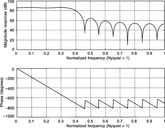
Figure 5.11
The magnitude response of the scaled filter is shown in Fig. 5.12 and now agrees closely with the filter specification. It follows that our filter has the transfer function of:
N.B. It is no coincidence that we are sampling at 20 kHz and that we needed to scale by 1/20 000. It is possible to show that, to derive the filter coefficients from the sampled unit impulse response values, we need to divide the sampled values by the sampling frequency.

Figure 5.12
So, to summarize: the starting point in the design process is the required frequency response of the filter. The IFT is then taken of this frequency response to generate the filter unit impulse response. An adequate time window is now chosen, with the central peak of the unit impulse response at its mid-point. The selected section of the unit impulse response is then shifted, sampled symmetrically, and the samples scaled. These scaled values are the filter coefficients.
A quicker approach
To make the principles behind the design process as clear as possible, the filter design has been approached in the most logical way. We started with the required frequency response and then used the IFT to convert to the time domain to get the corresponding unit impulse response. The unit impulse response was then sampled, shifted and finally scaled to find the FIR filter coefficients. However, this is rather a lengthy process and a much more direct and practical way of finding the coefficients follows.
We know that the unit impulse response is given by f(t) = (sin(2πfct))/πt from equation (5.2), and so the sampled values, before shifting and scaling, are given by:
However, we know that to get the filter coefficients, C(n), we need to scale these samples by dividing by fs.
But fsT = 1,
It is often more convenient to express the cut-off frequency in the normalized form, i.e. as a fraction of the Nyquist frequency, fN, and so we can rewrite the equation for C(n) as:
But 2fNT = fsT = 1,
By making this our starting point and, for our particular example, using n = −10 to +10, we can find the filter coefficients very quickly. We do not have to bother to time-shift the expression as long as we remember that C(−10) will correspond to our first coefficient, C(−9) to the second, etc. Neither is scaling necessary as this has been incorporated into the expression for C(n).
5.7 WINDOWING AND THE GIBBS PHENOMENON
Although the filter we have just designed satisfies the specification quite well, you will have noticed the ‘ripples’ in the stopband (Fig. 5.12). Much more seriously, these are also present in the passband, although they are less obvious because of the log scale. Figure 5.13 shows an expanded version of just the passband – the ripple is now much more apparent. This ripple in the passband is obviously undesirable as, ideally, we require a constant gain over this frequency range.
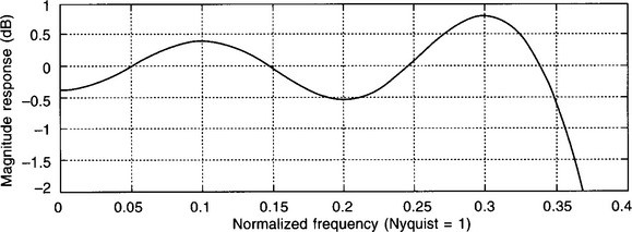
Figure 5.13
This rippling is termed the ‘Gibbs’ phenomenon, after an early worker in the field of signal analysis. It occurs because we have applied a ‘window’ to the unit impulse response, i.e. we only considered that portion of the signal contained within the time-slot of 10−3 s.
In the previous example we have effectively applied a rectangular window, in that all signal values were multiplied by 1 over the 10−3 s time slot and by 0 for all other time values. There are, however, other standard window profiles available to us which we can use to reduce the ripple. One that is widely used is the Hamming window. The profile of this particular window is defined by:
where n is the sample number and N the total number of samples. The Hamming window profile, for N = 21, is shown in Fig. 5.14.

Figure 5.14
What we have to do is multiply all of the sampled values within the 10−3 s time slot by the corresponding window value, before we find our filter coefficients. More conveniently, this is equivalent to just multiplying each of our ‘raw’ filter coefficients by the Hamming window values.
The Hamming window values and the new filter coefficients for our lowpass filter are given in Table 5.2.
Table 5.2
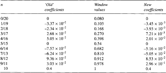
The response for the new filter is shown in Fig. 5.15. Applying the Hamming window has clearly been a success as the ripple in the passband is greatly reduced compared to Fig. 5.13.
| N.B.1 | There are several other window profiles which are commonly used. For example: |
| N.B.2 | The MATLAB function ‘fir1’ will generate FIR filter transfer function coefficients – the Hamming window function is automatically included. For example, all that is needed to design our lowpass filter is the single instruction:
where the ‘20’ is the number of coefficients less 1, and the ‘0.4’ is the normalized cut-off frequency, i.e. fc/fN. |
5.8 HIGHPASS, BANDPASS AND BANDSTOP FILTERS
We have shown that the coefficients for a linear-phase lowpass FIR filter are given by:

Figure 5.15
But what if we need a highpass filter?
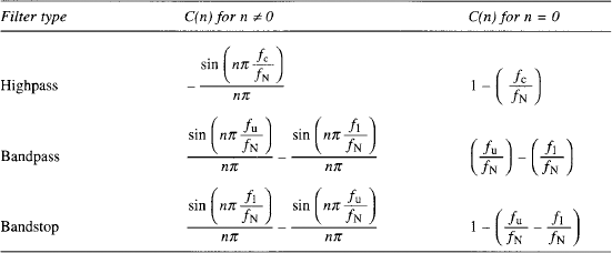
In Chapter 4, a lowpass IIR filter was converted to a highpass IIR filter by applying a particular transform in the z-domain (Section 4.17). We could do this here but it would be an unenviable task as there are so many z terms to transform. Also, even if we bothered, we would end up with an IIR filter, and one with a non-linear phase response. However, all is not lost, as it can be shown that the unit sample responses, and so the filter coefficients, for linear-phase highpass, bandpass and bandstop FIR filters are as shown in Table 5.3, where fu is the upper cut-off frequency and f1 the lower. If you require more details of the origin of these expressions see Chassaing and Horning (1990).
Table 5.3
Highpass, bandpass and bandstop filters, with a variety of window functions, can also be designed using the MATLAB, ‘fir1’ function. Refer to the MATLAB user manual or help screen for further details.
5.9 SELF-ASSESSMENT TEST
(a) Design a lowpass FIR filter with a cut-off frequency of 3 kHz. The filter is to be used with a sampling frequency of 12 kHz and is to have a ‘length’ of 11, i.e. 11 coefficients are to be used.
(b) Redesign the filter, so as to reduce the passband ripple, by using a Hanning (N.B. not Hamming!) window.
2. Design a highpass FIR filter with cut-off frequency of 4 kHz. The filter is to be used with a sampling frequency of 20 kHz. A rectangular window is to be applied and 21 samples are to be taken. (Hint: Most of the groundwork has already been done during the design of the lowpass filter in Section 5.6.)
5.10 RECAP
• To design an FIR lowpass filter, using the Fourier (or windowing) method, we need to find the filter coefficients, C(n), by using
We are effectively sampling, shifting and scaling the unit impulse response of the desired filter.
• If necessary, in order to reduce passband (and stopband) ripple, i.e. the ‘Gibbs phenomenon’, a suitable window function (other than rectangular) can be applied.
• Expressions also exist for deriving the transfer function coefficients for highpass, bandpass and bandstop filters.
5.11 THE DISCRETE FOURIER TRANSFORM AND ITS INVERSE
The Fourier and inverse Fourier transforms were reviewed in Section 5.5. This was because the ‘Fourier’, or ‘windowing’, method of designing FIR filters relied heavily on the inverse Fourier transform. The other common design method is based on a variation of the inverse Fourier transform, termed the discrete inverse Fourier transform. A few pages on this transform are therefore in order.
Like the ‘normal’ or continuous Fourier transform, the discrete Fourier transform (DFT) allows us to find the frequency components that make up a signal. However, there is a major difference in that the DFT is an approximation as it converts a sampled time signal into the corresponding sampled frequency spectrum. In other words, the frequency spectrum derived from the sampled signal is defined only at particular frequency values. If the sampling frequency is fs, and N signal samples are taken, then the frequency spectrum generated by the DFT will consist only of frequencies of kfs/N, where k = 0 to N − 1. For example, if we sampled a signal at 5 kHz and we took just 10 samples, then the amplitude spectrum unravelled by the DFT might look like Fig. 5.16, i.e. only the amplitudes of the signal components at 0, 500, 1000, 1500, …, 4500 Hz will be revealed. The ‘step’ frequency of 500 Hz, (fs/N), is called the frequency resolution.

Figure 5.16
Also note the symmetry of the amplitude spectrum about the Nyquist frequency of 2.5 kHz. All discrete amplitude spectra, resulting from the spectral analysis of sampled signals, exhibit this symmetry. To understand the symmetry, imagine that the sequence is the output from a discrete filter, in response to an input of a unit sample function. As the z-transform of the output Y(z) = 1 × T(z), then the sampled spectrum of the signal must be the same as the sampled frequency response of the filter, i.e. the DFTs of the two must be the same. Now imagine the ‘frequency point’ moving in an anticlockwise direction around the unit circle of the p–z diagram for the filter transfer function. When the frequency point passes the Nyquist frequency the amplitude spectrum must begin to repeat itself, due to the symmetry of the p–z diagram about the real axis. For this reason, the Nyquist frequency is sometimes referred to as the ‘folding’ frequency.
Anyway – back to the main story.
Sampled frequency components are just what we need when we are processing frequency data by means of a computer, and so the DFT serves this purpose very well. However, a word of caution. If anything unusual is happening between the sampled frequencies then this will be missed when the DFT is applied. For example, let’s say that there is a ‘spike’ in the amplitude spectrum at a frequency of 660 Hz. If we are sampling at 5 kHz, and taking 10 samples as before, then this spike will fall between the displayed, sampled frequencies of 500 Hz and 1 kHz and so will not be revealed. Clearly, the more samples taken, the better the frequency resolution and so the less that will be missed, i.e. the more closely the DFT will approximate to the ‘normal’ or continuous Fourier transform.
As might be expected, the inverse discrete Fourier transform (IDFT) performs the opposite process, in that it starts with the sampled frequency spectrum and reconstructs the sampled signal from it. It is the IDFT which will be of particular use to us when we move on to the next design method.
The discrete Fourier transform (sampled time to sampled frequency) is defined by:
where Xk is the kth value of the frequency samples.
The inverse discrete Fourier transform (sampled frequency to sampled time) is defined by:
where x[n] is the nth sample in the sampled signal.
To make more sense of these two very important transforms it’s best to look at an example.
Example 5.1
Use the DFT to find the sampled frequency spectrum, both magnitude and phase, of the following sequence: 2, −1, 3, given that the sampling frequency is 6 kHz. When the sampled spectrum has been derived, apply the inverse DFT to regain the sampled signal.
Solution: As we are sampling at 6 kHz, and taking three samples (very unrealistic but O.K. to use just to demonstrate the process), the frequency resolution is 6/3 (fs/N), i.e. 2 kHz. Therefore the DFT will derive the sampled spectrum for frequency values of 0, 2 and 4 kHz (kfs/N for n = 0 to N − 1, where N = 3).
We now need to apply the DFT to find the sampled frequency spectrum, both magnitude and phase. Therefore, using

Using Euler’s identity:

The magnitude and phase values are shown in Fig. 5.17.

Figure 5.17
N.B. As explained earlier in this section, the magnitudes at 2 and 4 kHz should be the same, i.e. symmetric about the Nyquist frequency of 3 kHz – the difference is due to approximations made during calculation. Similarly, the phase angles should have inverted symmetry, in other words, have the same magnitudes but with opposite signs.
We should now be able to process these three sampled frequency values of 4∠0, 3.58∠74.1° and 3.65Z∠− 73.1° using the IDFT, to get back to the three signal samples of 2, −1 and 3.

(Assuming that the relatively small imaginary part is due to approximations made during the maths, which seems a reasonable assumption. Note that this is the first signal sample.)
Missing out the next few lines of complex maths (which you might wish to work through for yourself), and ignoring small approximation errors, we end up with x[1] = −1.

Leaving out the intervening steps, and again ignoring small rounding errors, we get x[2] = 3, which agrees with the final signal sample.
5.12 THE DESIGN OF FIR FILTERS USING THE ‘FREQUENCY SAMPLING’ METHOD
The starting point for the previous ‘Fourier’ or ‘windowing’ design method (Section 5.6), was the required frequency response. The IFT was then applied to convert the frequency response to the unit impulse response of the filter. The unit impulse response was then shifted, sampled and scaled to give the filter coefficients.
The ‘frequency sampling’ method is very similar but the big difference here is that the starting point is the sampled frequency response. This can then be converted directly to the FIR filter unit sample response, and so to the filter coefficients, by using the IDFT.
To demonstrate this approach we will design a lowpass FIR filter with a cut-off frequency of 2 kHz – the filter being used with a sampling frequency of 9 kHz. Therefore fc = 0.444 fN.
The required magnitude response of the filter is shown in Fig. 5.18. For the purpose of demonstrating this technique the frequency has been sampled at just nine points, starting at 0 Hz, i.e. every 1 kHz. Note that fs is not one of the sampled frequencies. To understand this, look back to Example 5.1, where a sampled time signal was converted to its corresponding sampled frequency spectrum using the DFT. By doing this, only frequencies up to (N − 1)fs/N were generated, i.e. the sampled frequency spectrum stopped one sample away from fs. As would be expected, by using the IDFT to process these frequency samples, the original signal was reconstituted. With the frequency sampling method, we start with the sampled frequency response, stopping one sample short of fs, and aim to derive the equivalent sampled time function by applying the IDFT. As explained in Section 5.6, this time function will be the filter unit sample response, i.e. Y(z) = 1 × T(z), and so the IDFT of T(z) must be the IDFT for Y(z). These sampled signal values must also be the FIR filter coefficients.

Figure 5.18
The frequency samples for the required filter, derived from Fig. 5.18, are shown in Table 5.4.
Table 5.4
| n | |Xk| |
| 0 | 1 |
| 1 | 1 |
| 2 | 0.5 |
| 3 | 0 |
| 4 | 0 |
| 5 | 0 |
| 6 | 0 |
| 7 | 0.5 |
| 8 | 1 |
Two important points to note. The first is that the response samples shown in Table 5.4 are the magnitudes of the sampled frequency response, |Xk|, whereas the Xk in the expression for the IDFT, equation (5.6), also includes the phase angle.
The second point is that the samples at n = 2 and n = 7 are shown as 0.5 rather than 1 or 0. By using the average of the two extreme values, we will design a much better filter, i.e. one that satisfies the specification more closely than if either 1 or 0 had been used.
We will now insert our frequency samples into the IDFT in order to find the sampled values of the unit impulse response and, hence, the filter coefficients. However, before we do this, a few changes will be made to the IDFT, so as to make it more usable.
At the moment our IDFT is expressed in terms of the complex values Xk, rather than the magnitude values, |Xk|, of Table 5.4. However, it can be shown that |Xk| and Xk are related by:
or ![]() for this particular example.
for this particular example.
N.B. This exponential format is just a way of including the phase angle, i.e.
(from Euler’s identity).
where ϕ is the phase angle.
Therefore the magnitude of the phase angle is
Although it’s not obvious, this particular phase angle indicates a filter delay of (N − 1)/2 sample periods. When we designed FIR filters using the ‘Fourier’ method in Section 5.6, we assumed zero phase before shifting, and then shifted our time response by (N − 1)/2 samples to the right, i.e. we effectively introduced a filter delay of (N − 1)/2 samples. This time-shifting results in a filter which has a phase response which is no longer zero for all frequencies but the new phase response is linear. In other words, by using this particular expression for the phase angle, we are imposing an appropriate constant filter delay for all signal frequencies. The exponential expression of ![]() is the same for all linear-phase FIRs that have a delay of (N − 1)/2 samples – which is the norm. For a fuller explanation, see Damper (1995).
is the same for all linear-phase FIRs that have a delay of (N − 1)/2 samples – which is the norm. For a fuller explanation, see Damper (1995).
Therefore, replacing Xk with ![]() , in the IDFT (equation (5.6)), where α = (N − 1)/2:
, in the IDFT (equation (5.6)), where α = (N − 1)/2:
Therefore, from Euler’s identity:
Further, as x[n] values must be real, i.e. they are actual signal samples, then we can ignore the imaginary ‘sin’ terms.
Finally, as all X terms, apart from X0, are partnered by an equivalent symmetric sample, i.e. |X1| = |X8|, |X2| = |X7| etc. (Fig. 5.18), then we can further simplify to:

We now only have to sum between k = 1 and k = (N − 1)/2 rather than 0 and (N − 1) and so avoid some work! In our example this means summing between 1 and 4 rather than 0 and 8.
To recap, we can use equation (5.7) to find the values, x[n], of the filter unit sample response. These values are also the FIR filter coefficients.
O.K – so let’s use equation (5.7) to find the filter coefficients. Substituting n = 0 and α = (9 − 1)/2 = 4 into equation (5.7), and carrying out the summation:
As |X3| and |X4| = 0 we only have two terms to sum.
Check for yourself that x[3] = 0.3006 and x[4] = 0.4444.
N.B. As we are designing a linear-phase filter, then the signal samples must be symmetric about the central value, x[4], i.e. x[0] = x[8], x[1] = x[7], etc., and so we only need to find the five x[n] values, x[0] to x[4].
It follows that the nine samples of the filter unit sample response are:
and, as these must also be our filter coefficients:

or
Figure 5.19 shows the frequency response of our filter and it looks pretty good. The cut-off frequency is not exactly the 2 kHz (0.444fN) required, but it’s not too far away. To be fair, to save too much mathematical processing getting in the way of the solution, far too few frequency samples were used. If we had taken a more realistic number of frequency samples than nine then the response would obviously have been much better.
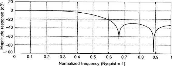
Figure 5.19
Here we used an odd number of frequency samples. The expression for the IDFT for an even number of samples is given in equation (5.8a). For completeness, the expression for an odd number is repeated as equation (5.8b).

The ‘even’ expression is the same as for an odd number of samples apart from the k range being from 1 to (N/2) − 1 rather than 1 to (N − 1)/2. If you inspect equation (5.8a) you will notice that the N/2 sample is not included in the IDFT. For example, if we used eight samples, then X0, X1, X2 and X3 only would be used, and not X4. I won’t go into this in any detail but using an even number of samples does cause a slight problem in terms of the N/2 frequency term. One solution, which gives acceptable results, is to treat XN/2 as zero – this is effectively what has been done in equation (5.8a). See Damper (1995) for an alternative approach.
5.13 SELF-ASSESSMENT TEST
A highpass FIR filter is to be designed, using the ‘frequency sampling’ technique. The filter is to have a cut-off frequency of 3 kHz and is to be used with a sampling frequency of 9 kHz. The frequency response is to be sampled every 1 kHz.
5.14 RECAP
• The discrete Fourier transform (DFT), is used to convert a sampled signal to its sampled frequency spectrum, while the inverse discrete Fourier transform (IDFT) achieves the reverse process.
• The sampled frequency spectrum obtained using the DFT consists of frequency components at frequencies of kfs/N, for k = 0 to N − 1, where fs is the sampling frequency and N the number of samples taken.
• By beginning with the desired sampled frequency response of a filter, it is possible to find the coefficients of a suitable linear-phase FIR filter by applying the IDFT.
5.15 THE FAST FOURIER TRANSFORM AND ITS INVERSE
Clearly, the discrete Fourier transform is hugely important in the field of signal processing as it allows us to analyse the spectral content of a sampled signal. The IDFT does the opposite, and we have seen how invaluable it is when it comes to the design of FIR filters. Although we will not be looking at this particular method, the DFT can also be used to design digital filters.
However, as useful as they are, the DFT and its inverse have a major practical problem – this is that they involve a great deal of computation and so are very extravagant in terms of computing time. Earlier, we performed some transforms manually, using unrealistically small numbers of samples. Imagine the computation needed if thousands of samples were to be used – and this is not unusual in practical digital signal processing. Because of this, algorithms have been developed which allow the two transforms to be carried out much more quickly – very sensibly they are called the fast Fourier transform (FFT), and the fast inverse Fourier transform (FIFT) or inverse fast Fourier transform (IFFT). Basically, these algorithms break down the task of transforming sampled time to sampled frequency, and vice-versa, into much smaller blocks – they also take advantage of any computational redundancy in the ‘normal’ discrete transforms.
To demonstrate the general principles, the FFT for a sequence of four samples, x[0], x[1], x[2] and x[3], i.e. a ‘four point’ sequence, will now be derived.
or, more neatly:
where ![]() . (W is often referred to as the ‘twiddle factor’!)
. (W is often referred to as the ‘twiddle factor’!)
This set of four equations can be expressed more conveniently, in matrix form, as:

Expanding W1, W2, W3 etc. using Euler’s identity, or by considering the periodicity* of these terms, you should be able to show that:
Substituting into equation 5.9:

Expanding the matrix equation:
If we now let:
then:
When carried out by a computer, the process of multiplication is much more time consuming than the process of addition and so it is important to reduce the number of multiplications in the algorithm as much as possible. We have clearly done this and so the computation of X0 to X3 should be achieved much more quickly than if the DFT were to be used.
The FFT, represented by the four equations (5.11a–d) above, can be depicted by the signal flow diagram of Fig. 5.20. These FFT signal flow diagrams are often referred to as ‘butterfly’ diagrams for obvious reasons.
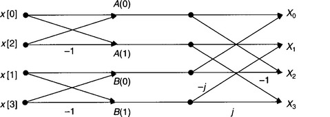
Figure 5.20
We have looked at the FFT for just four samples but the FFT exists for any number of samples (although the algorithm is simplest for an even number). Indeed, the relative improvement in processing time increases as N increases. It can be shown that the number of multiplications performed by the normal DFT, when transforming a signal consisting of N samples, is of the order of N2, whereas, for the FFT, it is roughly N log2N. For our four-sample sequence this corresponds to approximately 16 multiplications for the DFT and eight for the FFT. However, if we take a more realistic number of samples, such as 1024, then the DFT carries out just over one million multiplications and the FFT just over 10 000, i.e. a much more significant difference. See Proakis and Manolakis (1996), Lynn and Fuerst (1994), or Ingle and Proakis (1997) if you require a more detailed treatment of this topic.
N.B. We are spending time looking at the FFT and its inverse, the IFFT, because these transforms are used in the design of digital signal processing systems. However, before moving on from the FFT it should be pointed out that digital signal processors, in turn, are used to find the FFT of a signal and so allow its spectrum to be analysed. This is a very common application of DSP systems.
The fast inverse Fourier transform
So far we have concentrated on the FFT but the fast inverse Fourier transform is equally important. As it is the inverse process to the FFT, basically, all that is needed is to move through the corresponding FFT signal flow diagram in the opposite direction. However, it can be shown that we first need to change the signs of the exponentials in the W terms – in other words, change the sign of the phase angle of the multipliers. As phase angles of ±180°, ±540°, ±900° etc. are effectively the same, as are ±0°, ±360°, ±720° etc. then all that is needed is to change the sign of the j multipliers. This is because unit vectors with phase angles of ±90° or ±270° etc., are not the same, one is represented on an Argand diagram by j and the other by –j.
It can also be shown that the resulting outputs need to be divided by N.
Figure 5.21 shows the modified butterfly diagram for our four-sample system. Just to show that this works, consider x[0]. From Fig. 5.21:

Figure 5.21
but A(0) = X2 + X0 and A(1) = X1 + X3
Substituting for X0, X1, X2 and X3 using equations 5.10 (a–d), you should find that you end up with x[0] = x[0], which shows that the algorithm represented by Fig. 5.21 works! (See Damper (1995) and also Ifeachor and Jervis (1993) for further details.)
5.16 MATLAB AND THE FFT
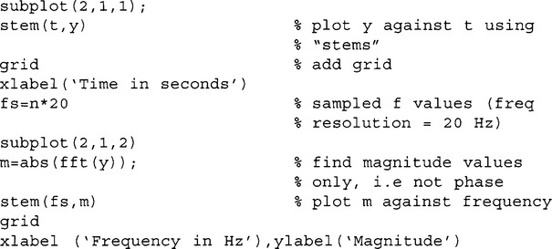
The FFT for a sequence can be obtained very easily by using the MATLAB, ‘fft’ function. The following program will generate the sampled, complex frequency values for the 10 sample sequence 1, 2, 3, 5, 4, 2, −1, 0, 1, 1.

The sampled magnitude and phase values are displayed graphically in Fig. 5.22, using a sampling frequency of 10 kHz.

Figure 5.22
More interestingly, Fig. 5.23(a) shows the sampled signal produced by adding three sine waves of unit amplitude, having frequencies of 100, 210 and 340 Hz, while Fig. 5.23(b) displays the sampled amplitude spectrum, obtained using the ‘fft’ function. The sampling frequency used was 1 kHz and 50 samples were taken and so the frequency resolution is 20 Hz, (fs/N). Note that the signals of frequencies 100 and 340 Hz show up very clearly in Fig. 5.23(b), while the 210 Hz signal is not so obvious. This is because 100 and 340 Hz are two of the sampled frequencies, i.e. nfs/N, while 210 Hz is not. Even so, the fft makes a valiant attempt to reveal it!
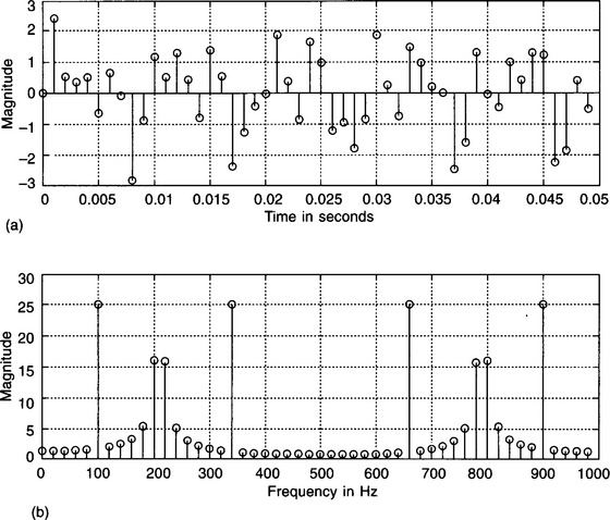
Figure 5.23

There is also a MATLAB ‘ifft’ function. The following simple program shows how the 10-point sequence, 1, 2, 3, 5, etc., ‘fft’d’ earlier, can be recovered by using the ifft function.
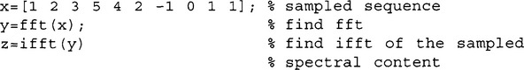
The results obtained are:
![]()
i.e. the original real, sampled signal of 1, 2, 3, 5, etc. is revealed by the ifft function.
5.18 A FINAL WORD OF WARNING
In this book we have been looking at the theory behind the analysis and design of digital filters. However, when you tackle some practical processing you might find that the system doesn’t perform quite as expected! The serious problem of pole and zero ‘bunching’ was mentioned in the previous chapter, but there are many other sources of error which could affect the behaviour of digital signal processing systems. One obvious cause of inaccuracies is the quantization of the input signal due to the A-to-D converter. The digital output values of the converter will only be approximate representations of the continuous input values – the smaller the number of A-to-D bits the more this quantization error. Further errors are introduced because the processor registers have a finite number of bits in which to store the various data, such as input, output and multiplier values. This will result in numbers being truncated or rounded. These errors will be catastrophic if, as a result of an addition or a multiplication for example, the resulting values are just too big to be stored completely. Such an overflow of data usually results in the most significant bits being lost and so the remaining stored data are nonsense. To reduce the risk of this, the processing software often scales data, i.e. reduces them. Under certain circumstances, the rounding of data values in IIR systems can also cause oscillations, known as ‘limit cycles’.
This is just a very brief overview of some of the more obvious shortcomings of DSP systems. If you would like to learn more about this aspect of digital signal processors then some good sources are Jackson (1996), Proakis and Manolakis (1996), Terrell and Lik-Kwan Shark (1996) and Ifeachor and Jervis (1993).
5.19 CHAPTER SUMMARY
In this, the final chapter, a case for using FIR rather than IIR filters was made. The major advantage of FIR systems is that it is possible to design them to have linear phase characteristics, i.e the phase shift of any frequency component, caused by passing through the filter, is proportional to the frequency. These linear-phase filters effectively delay the various signal frequency components by the same time, and so avoid signal distortion. For an FIR filter to have a linear phase response, it must be designed to have symmetric transfer function coefficients.
Apart from it being impossible for an FIR filter to be unstable (unlike IIR filters), a further advantage is that they can be designed to have a magnitude response of any shape – although only ‘brickwall’ profiles have been considered here.
Two major design techniques were described – the ‘Fourier’ or ‘windowing’ method and also the ‘frequency sampling’ approach. The improvement in filter performance, resulting from the use of a suitable ‘window’ profile, such as Hamming, Hanning or Blackman, was also discussed and demonstrated.
As the two design methods rely heavily on either the continuous or the discrete Fourier transforms – or their inverses, these topics were also covered. The problem of the relatively long processing time required by the DFT and IDFT was then considered and the alternative, much faster FFT and FIFT described.
Finally, some of the more obvious sources of filter error were highlighted.
5.20 PROBLEMS
1. A lowpass FIR filter is to be designed using the ‘Fourier’ or ‘windowing’ method. The filter should have 11 coefficients and a cut-off frequency of 0.25fN. The filter is to be designed using (a) a rectangular window and (b) a Hamming window.
2. A bandpass FIR filter, of length nine (nine coefficients) is required. It is to have lower and upper cut-off frequencies of 3 and 6 kHz respectively and is intended to be used with a sampling frequency of 20 kHz. Find the filter coefficients using the Fourier method with a rectangular window.
3. A discrete signal consists of the finite sequence 1, 0, 2. Use the DFT to find the frequency components within the signal, assuming a sampling frequency of 1 kHz. Check that the transformation has been carried out correctly by applying the IDFT to the derived frequency components in order to recover the original signal samples.
4. Use the ‘frequency sampling’ method to design a lowpass FIR filter with a cut-off frequency of 500 Hz, given that the filter will be used with a sampling frequency of 4 kHz. The frequency sampling is to be carried out at eight points. (N.B. An even number of sampling points.)
5. A bandstop filter is to be designed using the frequency sampling technique. The lower and upper cut-off frequencies are to be 1 and 3 kHz respectively and the filter is to be used with a sampling frequency is 9 kHz. The frequency sampling is to be carried out at nine points.
6. A discrete signal consists of the four samples 1, 2, 0, −1.
*Periodicity: Remember that ejθ represents a unit vector on the Argand diagram, inclined at an angle of θ to the positive real axis. It follows that ![]() and
and ![]() , i.e. W1 and W9, only differ in that W9 has made two extra revolutions. Effectively, they both represent unit vectors inclined at −90°, or +270°, to the positive real axis, and so they are equal to –j.)
, i.e. W1 and W9, only differ in that W9 has made two extra revolutions. Effectively, they both represent unit vectors inclined at −90°, or +270°, to the positive real axis, and so they are equal to –j.)